A Sharp-Interface Immersed Boundary Method forSimulating High-Speed Compressible InviscidFlowsJunjie Wang 

Nanjing University of Aeronautics and AstronauticsXiangyu Gu 

China Academy of Launch Vehicle TechnologyJie Wu  ( wuj@nuaa.edu.cn )

Nanjing University of Aeronautics and Astronautics

Research

Keywords: immersed boundary method, inviscid compressible �ows, sharp interface, shock waves,OpenFOAM

Posted Date: September 17th, 2020

DOI: https://doi.org/10.21203/rs.3.rs-47580/v2

License: This work is licensed under a Creative Commons Attribution 4.0 International License.  Read Full License

Version of Record: A version of this preprint was published on October 20th, 2020. See the publishedversion at https://doi.org/10.1186/s42774-020-00049-4.

1

A Sharp-Interface Immersed Boundary Method for

Simulating High-Speed Compressible Inviscid Flows

Junjie Wang1, Xiangyu Gu2, Jie Wu1, 3*

1. Department of Aerodynamics, Nanjing University of Aeronautics and Astronautics,

Yudao Street 29, Nanjing, Jiangsu 210016, China

2. China Academy of Launch Vehicle Technology,

Nandahongmen Street 1, Beijing 100076, China

3. Key Laboratory of Unsteady Aerodynamics and Flow Control, Ministry of Industry

and Information Technology, Nanjing University of Aeronautics and Astronautics,

Yudao Street 29, Nanjing, Jiangsu 210016, China

Abstract

This paper presents a robust sharp-interface immersed boundary method for

simulating inviscid compressible flows over stationary and moving bodies. The flow

field is governed by Euler equations, which are solved by using the open source

library OpenFOAM. Discontinuities such as those introduced by shock waves are

captured by using Kurganov and Tadmor divergence scheme. Wall-slip boundary

conditions are enforced at the boundary of body through reconstructing flow variables

at some ghost points. Their values are obtained indirectly by interpolating from their

mirror points. A bilinear interpolation is employed to determine the variables at the

mirror points from boundary conditions and flow conditions around the boundary. To

* Corresponding author; Email: wuj@nuaa.edu.cn.

2

validate the efficiency and accuracy of this method for simulation of high-speed

inviscid compressible flows, four cases have been simulated as follows: supersonic

flow over a 15° angle wedge, transonic flow past a stationary airfoil, a piston moving

with supersonic velocity in a shock tube and a rigid circular cylinder lift-off from a

flat surface triggered by a shock wave. Compared to the exact analytical solutions or

the results in literature, good agreement can be achieved.

Keywords: immersed boundary method; inviscid compressible flows; sharp

interface; shock waves; OpenFOAM;

1. Introduction

Inviscid flows are usually used as flow field conditions for fast transient

problems, such as the impact of shock waves onto a structure [1-4] and the internal

flow field arising within a solid rocket motor [5]. To treat such problems, the

conventional body-conformal grid methods [6, 7] can be utilized. Although it is direct

to enforce boundary conditions on the fluid-structure interface with a body-conformal

grid method, the complex-shaped structure increases too much work on the grid

generation process. Moreover, a re-meshing algorithm is required to adapt a moving

solid boundary which consumes more computing time and increases the algorithmic

complexity of these body-conformal grid methods. For using a non-conforming

Cartesian grid, on the other hand, the immersed boundary method (IBM) has gained

attention as an appropriate method for tackling flows with complex-shaped stationary

or moving boundaries during last two decades. Applying the advantage of Cartesian

grid, in particular, some high-order algorithms for complicated moving problems have

3

been developed [8, 9].

It is well known that the IBM was firstly proposed by Peskin [10] to simulate the

blood flow in the heart. Following the pioneer work of Peskin, numerous scientists

have contributed to improve the accuracy and efficiency of the IBM. Huang et al. [11]

introduced the variety of IBM fundamentals and assessed the latest progresses

especially the strategies to address the challenges and the applications of the IBM.

According to the work of Cui et al. [12], the IBM can be classified into two categories,

namely diffused-interface methods and sharp-interface methods based on the

representation of the fluid-structure interface. The diffused-interface IBM can be

regarded as a continuous forcing approach. The boundary is smeared by distributing a

forcing term [11, 13] and a source term [14] to the surrounding Cartesian grid points

via a delta function [15]. After that, these two terms are added to the momentum

equation and energy equation, respectively. Our previous work [16] developed an

implicit diffused-interface IBM based on variable correction for simulating

compressible viscous flows over stationary and moving bodies. Furthermore, Wang et

al. [17] applied a diffused-interfaced IBM to simulate compressible multiphase flows.

The significant advantage of diffused-interface IBM is that it is formulated

independent of the spatial discretization, and it simplifies the implementation into an

existing fluid solver, just like [13, 14]. However, Sotiropoulos and Yang [18]

indicated that the classic diffused-interface IBM is difficult to simulate fluid-structure

interaction problems, because the inherent stiffness of the forcing term may induce

numerical instabilities and spurious oscillations.

4

On the other hand, the sharp-interface IBM can be regard as a discrete forcing

approach, in which the boundary is precisely tracked. It includes cut-cell method [19,

20], Cartesian IB method [12, 21], and ghost-cell method [8, 9]. Among these

methods, the cut-cell method can obtain the clearest interface. The reason is that the

boundary divides grid cells into two sub-cells for the solid phase and fluid phase,

respectively. Therefore, the conservation of mass, momentum and energy can be

strictly enforced into the fluid phase. However, the complicated cell reshaping

procedure causes difficulties in simulating complex moving body problems. In the

Cartesian IB method, the fluid points with at least one neighboring point inside the

solid body are called IB points or forcing points. Reconstructing the flow variables at

these points and enforcing the boundary conditions can ensure the accuracy of the

flow field. The ghost-cell method is similar to the Cartesian IB method. The solid

points with at least one neighboring point inside the fluid domain are called ghost

points. The reconstruction procedure is done at these ghost points. Tran and Plourde

[5] used both the Cartesian IB method and the ghost-cell method to solve internal

flows. Although the Cartesian IB method and the ghost-cell method are less accurate

than the cut-cell method because of their implicit representation of the solid boundary,

point recognition procedure is easier than the cut-cell procedure, and the flux

calculation around the immersed boundary is also not necessary. Mittal et al. [22]

have shown the large potential of ghost-cell method for simulation of highly complex

moving body problems.

In the ghost-cell method, the flow variables at the ghost points cannot be

5

interpolated from the fluid field or the boundary conditions directly. Thus, an image

point can be considered, which is the mirror of ghost point along the normal direction

to the boundary and is always in the fluid domain. A body intercept point is the

midway point between ghost point and image point, which must be on the boundary.

Therefore, boundary conditions can be enforced on body intercept points directly. The

flow variables at ghost points are interpolated from corresponding image points and

body intercept points [5, 8, 9, 22]. A significant issue of ghost-cell method is the

accuracy of the interpolation procedure at image points from corresponding body

intercept points and fluid points. Shuvayan et al. [21] used an inverse distance

weighting interpolation method to reconstruct the flow variables. This scheme

preserves the local maxima and minima, which leads to a smooth reconstruction and

is more stable than a polynomial reconstruction. A linear interpolation method was

used in [5, 12] to reconstruct the values at IB points. Khalili et al. [9] used a bilinear

interpolation for two-dimensional problems, and Mittal et al. [22] used a trilinear

interpolation for three-dimensional problems similarly. Higher-order polynomials are

required for more accurate results, but they often lead to numerical instabilities, and

more information is needed to determine the polynomials. Qu et al. [8] listed four

polynomials for the interpolation: a linear, an incomplete quadratic (bilinear), a

complete quadratic and a cubic. They found that higher-order polynomials (e.g., a

cubic polynomial) required more interpolation points and the computational time may

significantly increase. Furthermore, they revealed that the complete quadratic

polynomial does not significantly improve the accuracy of their method but requires

6

more interpolation points than the incomplete quadratic polynomial. It is shown that

bilinear interpolation may be an expected scheme to reconstruct the flow variables.

In this work, we present a robust IBM to simulate high-speed compressible

inviscid flows over stationary and moving bodies. The Euler equations are discretized

on a Cartesian grid and solved by a segregated density-based solver, namely

rhoCentralFoam with Kurganov and Tadmor divergence scheme in the open source

library OpenFOAM. The sharp-interface IBM is adopted, which is a significant issue

in this work, because the exact location of shock waves has to be predicted. Khalili et

al. [9] developed a ghost-cell IBM to simulate viscous compressible flows, and a

bilinear interpolation was utilized to reconstruct the flow variables. However, it is

noted that only low Mach number flows were considered in their study and the

obtained conclusions were similar to that of incompressible flows. In this study, the

similar ghost-cell IBM is adopted for enforcing the boundary conditions in simulating

high-speed compressible inviscid flows. For a moving rigid object, moreover, the

Newton’s second law of motion is utilized to solve strong coupling between fluid and

structural within each time step. Because of inviscid flows, there is no viscous stress

or torque on solid surface and the rotational motion is not involved. To validate the

proposed method combined with OpenFOAM, two stationary cases are simulated:

supersonic flow over a 15° angle wedge and transonic flow past a stationary airfoil.

Then a moving piston and a lifting-off circular cylinder are simulated to validate the

current method for handling moving body problems. All the results are compared well

with the exact analytical solutions or the results in literature.

7

This paper is organized as follows. In Section 2, governing equations for fluid

flows and motions of rigid bodies are described. In Section 3, numerical methods are

presented, i.e., the governing equations in OpenFOAM and the ghost-cell IBM. In

Section 4, four cases are simulated to validate the efficiency and accuracy of this

method. In Section 5, conclusions are summarized.

2. Governing Equations

For flows over a stationary body, only the flow field should be resolved. But for

flows over a moving body, both the flow field and the motion of body should be

resolved. Moreover, the fluid is strongly affected by the existence of body, and the

body motions are coupled with the fluid flows.

2.1 Governing equations for fluid flows

For inviscid compressible flows, the Euler equations are solved, which can be

written as follows:

( ) 0t

+ =

u (1)

( ) ( ) 0pt

+ + =

u

uu (2)

( ) ( ) 0t

t

ee p

t

+ + =

u u (3)

where is the fluid density, u is the fluid velocity, and p is the pressure. In

addition, te is the total energy that includes kinetic energy and internal energy:

1 1

2 2t v

e e C T = + = + u u u u (4)

where e is the internal energy, vC is the heat capacity at constant volume, and T

8

is the fluid temperature. As the perfect gas is considered here, the equation of state

p RT= is adopted, where R is the specific gas constant.

The Mach number Ma is defined as U

MaRT

= , where U is the

freestream velocity, T is the freestream temperature, and is the specific heat

ratio, which is kept constant at 1.4 in present work. The pressure coefficient is defined

as ( ) 21/ 2

Bp

p pC

U

−= , where B

p is the pressure on the boundary of body, p is the

freestream pressure, and is the freestream density.

2.2 Governing equations for a passively moving rigid body

For a moving rigid body, only the velocity and the position vector of the mass

center ( cU , c

X ) are considered in this work. Due to the inviscid flows, the rotational

motion of the body is not involved since there is no existence of viscous stress or

torque. According to the Newton’s second law, the translational motion of a passively

moving rigid body can be solved by the following equations:

cc

d

dt=

XU (5)

cf

dm

dt= F

U (6)

where m is the mass of the body, and fF is the resultant force imparted by the

fluid to the body, which can be given by:

f fdS p dS

= = − f nF (7)

where ff represents the force per unit area on the boundary of body by the fluid,

which only includes the pressure interpolated from the flow fields, and represents

the boundary of body. ( ), tn = n X is the unit normal vector from the boundary into

9

the flow field, where X represents the position of the point on the boundary.

3. Numerical Methods

3.1 Basic solver in OpenFOAM

As mentioned in Introduction, an open source code, i.e. OpenFOAM, is used to

solve the governing equations of flow field. The codes in OpenFOAM are based on

cell-centered finite-volume method. High-speed compressible flows can be simulated

by the solver rhoCentralFoam, which is a semi-implicit segregated density-based

solver with the Kurganov-Tadmor divergence scheme [23]. More details about the

algorithmic structure of rhoCentralFoam solver can be found in Ref. [14]. In our

recent work [16], this solver has been combined with a diffused-interface IBM to

simulate viscous compressible flows. To extend this solver to deal with inviscid

compressible flows, only the viscous terms of the governing equations are ignored.

3.2 Boundary conditions

Classical boundary conditions including subsonic or supersonic inlet, subsonic or

supersonic outlet and walls are applied at the external boundaries of the computational

domain. For the inviscid flows, no boundary layer should develop in the vicinity of

the boundary of body. When a stationary body is considered, the traditional slip

boundary condition can be used on the boundary of body [5]. But when a moving

body is considered, the no-penetration boundary condition should be used. The

velocity vector ( ), tu X on the boundary is decomposed into the normal and

tangential velocity components:

10

( ) ( ) ( ), , ,t t t = n

u X u X n X (8)

( ) ( ) ( ), , ,t t t = u X u X X (9)

where ( ), tX is the unit tangential vector at X , which is perpendicular to the

unit normal vector. Considering the no-penetration boundary condition, these

components are then written as:

( ) ( ) ( ), ,ct t t = n

u X n XU (10)

( ),0

t

n

=

u X (11)

where the velocity of the body mass center ( )c tU has been introduced in the

previous section and it is independent of X for a rigid body.

For a stationary body, the pressure boundary condition / 0p n = can be

applied on the boundary. But it should be reformulated for a moving body. Following

the work of Udaykumar et al. [24], the pressure gradient normal to the boundary is

obtained by projecting the momentum equation into the boundary normal direction,

which results in:

( ) ( ) ( ),, ,

p t Dt t

n Dtt

= − = −

+

u u

nu n XuX

X (12)

where /D Dt is the material derivative. /D Dtu can be approximated directly

from the known boundary velocities and this obviates the approximation of the

convective term [8, 24].

In addition, an adiabatic boundary condition is applied at the boundary. The

temperature gradient normal to the surface is written as:

( ),0

T t

n

=

X

(13)

11

The boundary conditions above can be classified into two categories, Dirichlet

boundary condition (Eq. (10)) and Neumann boundary conditions (Eqs. (11-13)). In

our previous work [16], a variable correction-based IBM is developed to correct the

variables with the Dirichlet boundary condition, including the no-slip boundary

condition and the isothermal boundary condition. But it is difficult to handle the

Neumann boundary conditions. In this work, both two boundary conditions need to be

enforced into the proposed method.

3.3 Sharp-interface immersed boundary method

As one of sharp-interface immersed boundary methods, the ghost-cell IBM is

employed to impose the boundary conditions on the boundary of body in this work.

According to the location of boundary, the computational grid nodes lying inside the

body are identified as the solid points, and the nodes lying outside the body are

identified as the fluid points. Considering the rhoCentralFoam solver employed, one

layer of solid points adjacent to the immersed boundary are called ghost points (GPs),

as illustrated in Fig. 1. The interpolation procedure cannot be conducted on these GPs

directly. Thus, an image point (IP) is required, which is the mirror of GP along the

normal direction to the boundary. Thus, a boundary intercept (BI) point is defined as

the midway point between GP and IP. The unit normal vector n is also marked on

the BI point in Fig.1.

12

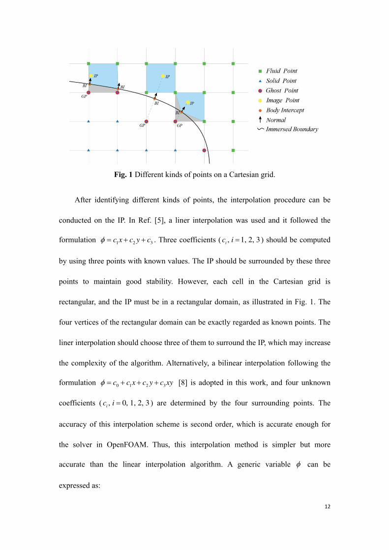
Fig. 1 Different kinds of points on a Cartesian grid.

After identifying different kinds of points, the interpolation procedure can be

conducted on the IP. In Ref. [5], a liner interpolation was used and it followed the

formulation 1 2 3c x c y c = + + . Three coefficients ( , 1, 2, 3i

c i = ) should be computed

by using three points with known values. The IP should be surrounded by these three

points to maintain good stability. However, each cell in the Cartesian grid is

rectangular, and the IP must be in a rectangular domain, as illustrated in Fig. 1. The

four vertices of the rectangular domain can be exactly regarded as known points. The

liner interpolation should choose three of them to surround the IP, which may increase

the complexity of the algorithm. Alternatively, a bilinear interpolation following the

formulation 0 1 2 3c c x c y c xy = + + + [8] is adopted in this work, and four unknown

coefficients ( , 0, 1, 2, 3i

c i = ) are determined by the four surrounding points. The

accuracy of this interpolation scheme is second order, which is accurate enough for

the solver in OpenFOAM. Thus, this interpolation method is simpler but more

accurate than the linear interpolation algorithm. A generic variable can be

expressed as:

13

TC = (14)

where 0 1 2 3, , ,T

C c c c c= is a coefficient vector, and 1, , ,T

x y xy = is

a coordinate vector that only depends on a local coordinate system ( ), x y . As

mentioned above, the coefficient vector C should be determined by four

surrounding points. However, if the surrounding point is just one GP, its

corresponding BI would be used. Then the interpolation domain changes from a

rectangle to the blue area in Fig. 1. The four surrounding points are marked as

, 0, 1, 2, 3i

P i = , which can be a fluid point or a BI point. Due to the particularity of

the BI point, Khalili et al. [9] considered multiple situations for interpolation

according to the number of the BI points in the interpolation domain. In the current

method, however, such complicated procedure is discarded, and only a judgment step

is required to determine the information type of a surrounding point. The flow

variables on the fluid point can be obtained from the flow field, while the values

on the BI point can be obtained by using the boundary conditions. The Dirichlet-type

boundary condition (Eq. (10)) is enforced on the BI point just like the fluid point. But

for the Neumann-type boundary conditions (Eqs. (11-13)), some modification is

required:

( )

( ) ( )1 3 2 3

0 1 2 3

, ,

, ,

0 ( )

x y

BI

x y

x y y x

n nn x y

c c y c c x n n

c n c n c xn yn c

=

= + +

= + + + +

(15)

where ( ), x y is the BI point coordinate, and ( ), x yn nn = is the unit normal vector

at the BI point.

14

The unknown coefficients C can be computed from the four surrounding points

with their flow information:

AC = (16)

1C A

−= (17)

where 0 1 2 3, , ,T

A = is a 4 4 matrix depending on the coordinate

information of the four surrounding points, and 0 1 2 3, , ,T = is a

generic variable vector. i and i

( 0, 1, 2, 3i = ) can be obtained by a judgment

step, based on the information type of i

P :

( )

( )

0, , ,

1, , ,

T

xi yi i yi i xi

iT

i i i i

Neumann boundary condn n x n y n itionat BI with

x y x y others

+ =

(18)

( )

( )

i

i

i

Neumann boundarat BI w yith conditionn

others

=

(19)

If iP is a BI point and the given boundary condition is the Neumann-type boundary

condition, Eq. (15) will be used.

Then the flow variables at the image point IP can be obtained as:

T

IP IPC = (20)

After obtaining the values at the IP, the flow variables at the GP can be

determined by using the boundary conditions on the immersed boundary. A linear

interpolation along the normal is employed. Different types of boundary conditions

need different formulas to calculate the values of flow variables at the GP:

( )

( )

2BI IP

GP

IP

BI

Dirichlet boundary condition

Neumann boundary conditionln

−= −

(21)

15

where l is the length of the normal probe from the GP to the IP.

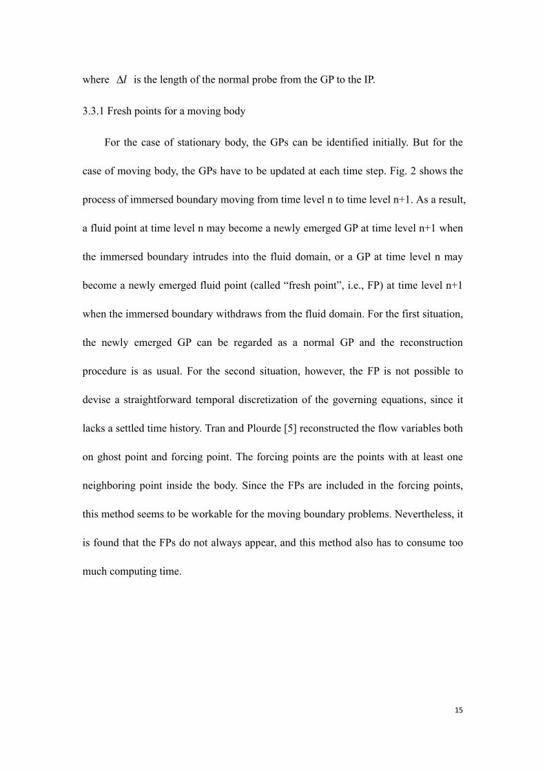
3.3.1 Fresh points for a moving body

For the case of stationary body, the GPs can be identified initially. But for the

case of moving body, the GPs have to be updated at each time step. Fig. 2 shows the

process of immersed boundary moving from time level n to time level n+1. As a result,

a fluid point at time level n may become a newly emerged GP at time level n+1 when

the immersed boundary intrudes into the fluid domain, or a GP at time level n may

become a newly emerged fluid point (called “fresh point”, i.e., FP) at time level n+1

when the immersed boundary withdraws from the fluid domain. For the first situation,

the newly emerged GP can be regarded as a normal GP and the reconstruction

procedure is as usual. For the second situation, however, the FP is not possible to

devise a straightforward temporal discretization of the governing equations, since it

lacks a settled time history. Tran and Plourde [5] reconstructed the flow variables both

on ghost point and forcing point. The forcing points are the points with at least one

neighboring point inside the body. Since the FPs are included in the forcing points,

this method seems to be workable for the moving boundary problems. Nevertheless, it

is found that the FPs do not always appear, and this method also has to consume too

much computing time.

16

Fig. 2 The emergence of fresh point due to the boundary motion from time level n to time level n+1.

In the present method, the reconstruction procedure on the FP is similar to that of

GP. The interpolation domain changes from a rectangle to the blue area in Fig. 2, as

the FP is shifted to its corresponding BI point. The other three surrounding points are

marked as , 1, 2, 3i

P i = , which can be confirmed by:

( ) ( )( )( ) ( )( )

( ) ( ) ( )( )

1 1

2 2

3 3

, ,

, ,

, ,

FP x FP

FP FP y

FP x FP y

x y x sign n x y

x y x y sign n y

x y x sign n x y sign n y

= + = + = + +

(22)

where ( ), i ix y represents the coordinate of the iP , sign is the symbolic function,

and , x y are the mesh steps. If iP is a FP, it will be also shifted to its

corresponding BI point. And this manipulation is similar to that of GP. The flow

variables are directly interpolated to the FP:

T

FP FPC = (23)

At each time step, the layer of FP is required to be one layer depth at least to

guarantee the success of interpolation step. Considering the motion of immersed

boundary and its velocity, the time step should be constrained as

17

( )min , / ct x y U .

It should be clarified that the current interpolation procedure has some general

similarities with the method proposed by Mittal et al. [22]. However, their

interpolation stencil was always in a rectangular domain and the surrounding points

would contain other GPs. As a result, a point Gauss-Seidel method was used for these

coupled GPs. In the current method, if the surrounding point is just one GP, its

corresponding BI point will replace it. Consequently, the surrounding points only

include fluid points or BI points in the current interpolation stencil, as illustrated in

Figure 1. Then, the flow variables at the GP can be computed easier. Another

advantage of the current method is that the BI points are included in the surrounding

points and the boundary information is enforced into the interpolation procedure. The

second difference is the reconstruction procedure of FPs. Mittal et al. [22] used the

same method as GPs to calculate FPs. When the FP is in the fluid domain, the current

method directly uses surrounding points to perform the interpolation to obtain the

flow variables at the FP. Therefore, the calculation process is more concise.

3.3.2 Computing the forces on the body

For inviscid flows, only the pressure acting on the surface of body is required to

be computed. The BI point is treated as an interpolation point, and the pressure BIp

can be achieved by using Eq. (10). Then Eq. (7) can be rewritten as:

f BI i i

i

p dS p s

= − = − F n n (24)

where is is the arc length of the immersed boundary around the BI point. The

pressure coefficient at the BI point can be expressed as:

18

( ) 21/ 2

BIp

p pC

U

−= (25)

3.4 Solution procedure

To summary, the solution procedure of the current algorithm from time level n to

n+1 is given as follows:

1) For a passively moving body, solve its motion and get cU , c

X by using Eqs.

(5) and (6); Otherwise, cU and c

X are given in advance.

2) Update the position of immersed boundary, and determine fluid points, solid

points, FPs, GPs, IPs, and BI points;

3) Calculate values of flow variables ( , p and Tu ) at FPs by using Eq. (23), and

then the density at FPs is updated by using the equation of state;

4) Calculate values of flow variables ( , p and Tu ) at GPs by using Eq. (21), and

then the density at GPs is updated by using the equation of state;

5) Solve the governing equations of flow field, and compute the flow variables by

using OpenFOAM;

6) Calculate the resultant force fF by using Eq. (24);

7) Repeat Steps 1 to 6 until convergence is reached, and obtain 1 1 1, , n n np + + +

u

and 1nT

+ .

4. Numerical Examples

4.1 Stationary cases

4.1.1 Supersonic oblique shock

To test the accuracy of the present method, a supersonic flow over a 15° angle

19

wedge is simulated. This flow can produce a supersonic oblique shock, which has an

exact analytical solution. Two Mach numbers are considered, i.e., 3.0Ma = and

5.0Ma = . Supersonic inlet and zero-gradient outlet are adopted. Initial conditions are

chosen with 1p Pa= and 1T K= .

Fig. 3 Pressure contours at 3.0Ma = .

In current simulations, the rectangular computational domain is ( )1.5 , 1.0m m . A

very fine uniform Cartesian grid is used with the mesh size of 1500 1000 , and then

the mesh spacing is 0.001h m = . At 3.0Ma = , the pressure contours are exhibited

in Fig. 3. The slope starts at 0.5x m= , where the supersonic flow forms an oblique

shock wave. The wave surface of the oblique shock is very clear, which is attributed

to the good ability of the current method to handle the supersonic flow over a body.

Table 1 Comparison of theoretical and present numerical results obtained from the supersonic oblique shock configuration.

Case Flow variables Exact Present

1 3.0Ma = 2Ma 2.255 2.255

2 1/p p 2.822 2.821

inlet outlet

15°

20

2 1/T T 1.388 1.388

Shock-angle 32.24° 32.21° 1 5.0Ma =

2Ma 3.504 3.504

2 1/p p 4.781 4.781

2 1/T T 1.736 1.736

Shock-angle 24.32° 24.31°

Table 1 lists the theoretical and numerical results from pre-shock state (subscript

1) and post-shock state (subscript 2): post-shock Mach number 2Ma , pressure ratio

2 1/p p , temperature ratio 2 1/T T , and shock-angle that is the angle between the

oblique shock and the horizontal plane. The present results are in agreement with the

exact solution, and the accuracy of the current method is well displayed.

To assess the convergence rate of the current method, the case at 3.0Ma = is

simulated with different meshes. Four uniform grids of 75 50 , 150 100 ,

300 200 and 1500 1000 are used. The corresponding grid steps are 0.02h m = ,

0.01h m = , 0.005h m = and 0.001h m = , respectively. As illustrated in Table 1,

the exact solution of shock-angle is =32.24 o . The error of shock-angle e versus

grid steps in the log scale is plotted in Fig. 4. From the figure, it is found that the slope

of the line is about 1.7. Although the accuracy of the interpolation scheme is second

order in the current IBM, some discrete schemes in the rhoCentralFoam solver are

only first-order. Therefore, the overall accuracy of the current solver is less than the

second-order.

21

Fig. 4 Convergence of numerical error versus grid step for supersonic oblique shock.

4.1.2 Transonic flow around a stationary airfoil

To verify the robustness of the present method, a flow around an

irregular-shaped object is simulated in this section. Here, a NACA0012 airfoil is

considered. Two transonic flows are selected, in which the free-stream Mach number

and angle of attack are: (a) 0.8, 1.25Ma = = o and (b) 0.85, 1Ma = = o . The

same problem has been simulated in previous work [25-27]. The computational

domain is 28 20c c with the mesh size of 511 251 , where c is the chord length

of airfoil, and the airfoil is located at ( )10 , 10c c . The region around the airfoil is

1.2 0.2c c , and a fine uniform mesh with the spacing of 0.005h c= is adopted.

h/m

e

10-4

10-3

10-2

10-110

-4

10-3

10-2

10-1

slope=1.7

22

(1) (2)

(3) (4)

Fig. 5 Pressure contours (1) and (3), Mach number contours (2) and (4), with different flows 0.8, 1.25Ma = = o (1-2) and 0.85, 1Ma = = o (3-4).

The pressure and Mach number contours are presented in Fig. 5. For the case of

0.8, 1.25Ma = = o , there are a relatively strong shock on the upper surface of the

airfoil and a weak shock on the lower surface of the airfoil, as illustrated in Figs. 5(1)

and 5(2). For the case of 0.85, 1Ma = = o , however, it is indicated that such

problem is not easy to be handled [25, 26]. The strong shock appears on both the

upper surface and the lower surface, as shown in Figs. 5(3) and 5(4).

23

(1) (2) Fig. 6 Pressure coefficient on the upper and lower airfoil surfaces compared to

reference results with different flows (1) 0.8, 1.25Ma = = o and (2)0.85, 1Ma = = o .

Fig. 6 shows the pressure coefficient pC− on the upper and lower airfoil

surfaces. From the figure, it can be found that the present results compare well with

the results of previous work [27, 28]. At 0.8, 1.25Ma = = o , the shock positions on

the upper and lower airfoil surfaces are accurately predicted. Although the case (b) is

difficult to simulate, the current method still can accurately predict the position of the

upper and lower surface shock waves.

Based on two problems above, the sharp-interface IBM in this study has been

proved to be able to deal with stationary boundary problems accurately.

4.2 Moving cases

4.2.1 Piston moving with supersonic velocity

x/c

-Cp

0 0.2 0.4 0.6 0.8 1-1.5

-1

-0.5

0

0.5

1

1.5

Upper_Present

Lower_Present

Upper_Liu and Hu

Lower_Liu and Hu

x/c

-Cp

0 0.2 0.4 0.6 0.8 1-1.5

-1

-0.5

0

0.5

1

1.5

Upper_Present

Lower_Present

Upper_Amaladas and Kamath

Lower_Amaladas and Kamath

24

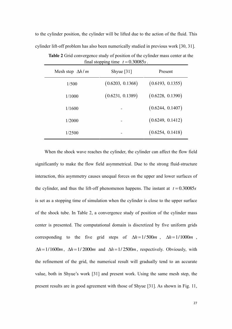
Fig. 7 Schematic diagram of piston movement.

To further validate the current method, the moving body problems will be

simulated. The first one is a piston moving at a constant speed of 2.0Ma = in a

quiescent fluid. The movement sketch is shown in Fig. 7. The thickness of the piston

is L , and it is located in the middle of a shock tube initially. The shock tube has a

length of 128L and a width of 4L . In the whole computational domain, the

parameters of the initial quiescent fluid are 0 /u v m s= = , 1p Pa= , and 1T K= .

Then the piston is given a sudden velocity with 2.0Ma = . The same problem has

also been simulated in previous studies [19, 20, 29], and it has an analytical solution.

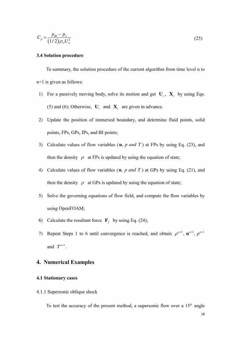
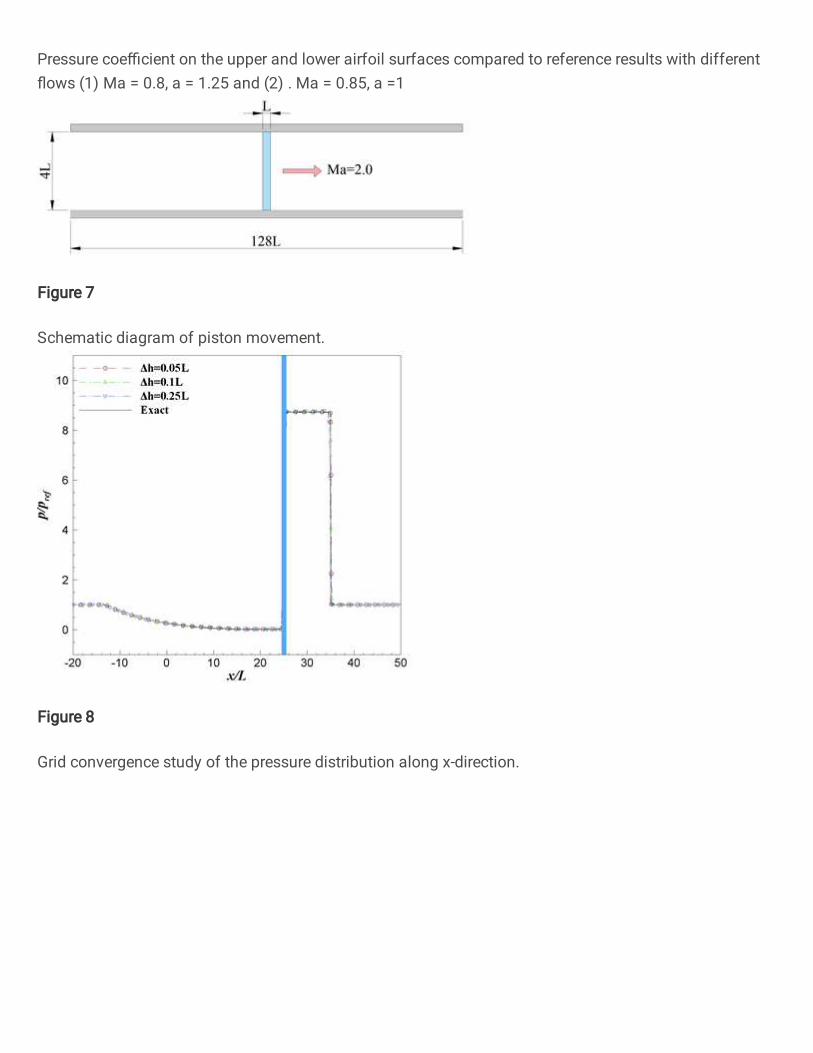
Fig. 8 Grid convergence study of the pressure distribution along x-direction.

25

The computational domain with the size of 128 4L L is discretized by using

three different uniform grids with 512 16 , 1280 40 and 2560 80 . These three

grids correspond to the three mesh steps of 0.25h L = , 0.1h L = and 0.05h L = ,

respectively. The computations are performed till the instant of 25 / pistont L u= , where

pistonu is the velocity of the piston. Fig. 8 shows the pressure distribution along

x-direction with different mesh steps. The piston is represented by a blue strip in the

figure. 1refp Pa= is the reference pressure. Obviously, the result from fine mesh is

closer to the exact solution than that from coarse mesh, especially at the corners of the

curve. However, even for the coarsest mesh, the calculated result is generally in good

agreement with the exact solution. Thus, it means that the current method has good

robustness, and the satisfactory result can be obtained even at a relatively coarse grid.

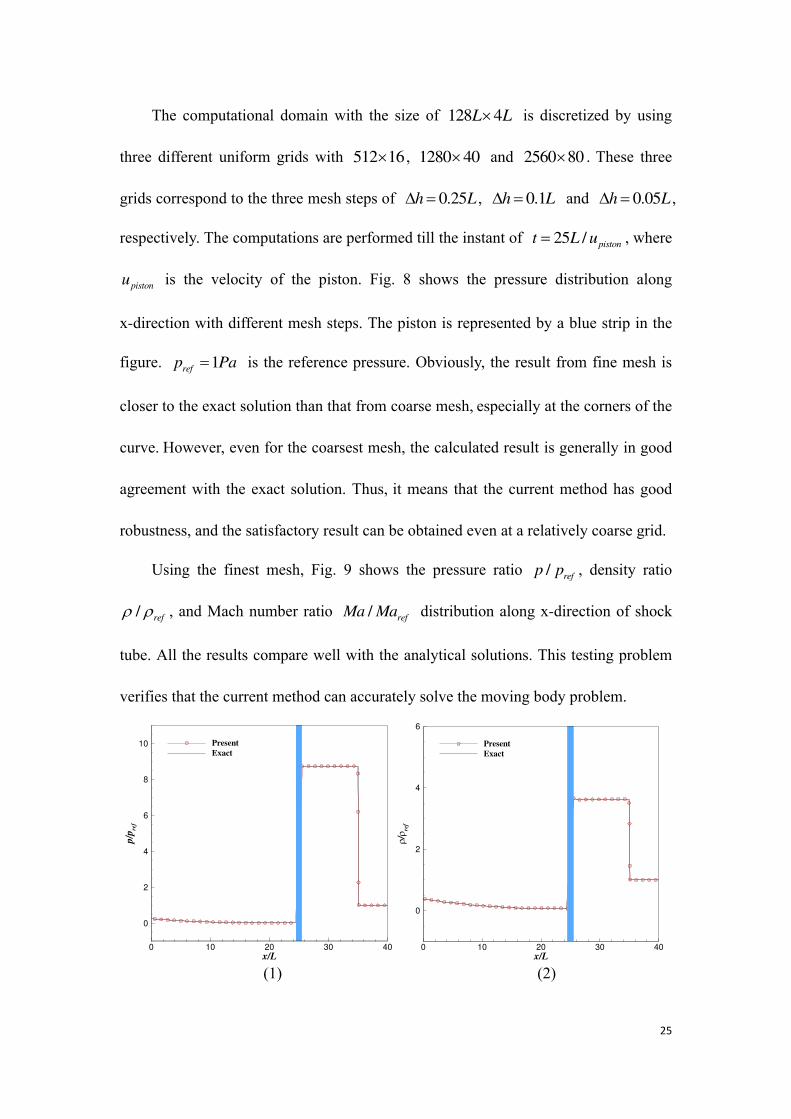
Using the finest mesh, Fig. 9 shows the pressure ratio /ref

p p , density ratio

/ ref , and Mach number ratio /ref

Ma Ma distribution along x-direction of shock

tube. All the results compare well with the analytical solutions. This testing problem

verifies that the current method can accurately solve the moving body problem.

(1) (2) x/L

p/p

ref

0 10 20 30 40

0

2

4

6

8

10 Present

Exact

x/L

/ r

ef

0 10 20 30 40

0

2

4

6

Present

Exact

26

(3)

Fig. 9 Comparison of (1) pressure, (2) density and (3) Mach number distribution along x-direction with analytical results at the finest mesh 0.05h L = .

4.2.2 Lift-off of a cylinder

Fig. 10 Schematic diagram of cylinder lift-off.

The second moving body problem to be simulated is a rigid cylinder whose

motion is induced by the fluid. This problem takes place in a shock tube, whose

domain size is 1 0.2m m , as illustrated in Fig. 10. At the initial moment, a shock

wave with Mach 3 is located at 0.08x m= , which is traveling from left to right. The

pre-shock state, which is on the right of the shock, is at rest with 1p Pa= , 1T K= ,

and 0 /u v m s= = . The flow variables at the post-shock state can be calculated from

the total temperature. The radius of rigid cylinder is 0.05m, which is at rest initially on

the floor of the shock tube. The center of the cylinder is initially at ( )0.15 , 0.05m m ,

and the density of the cylinder is 310.77 /kg m . When the Mach 3 shock wave moves

x/L

Ma/M

are

f

0 10 20 30 40

0

2

4

6

Present

Exact

27

to the cylinder position, the cylinder will be lifted due to the action of the fluid. This

cylinder lift-off problem has also been numerically studied in previous work [30, 31].

Table 2 Grid convergence study of position of the cylinder mass center at the final stopping time 0.30085t s= .

Mesh step /h m Shyue [31] Present

1/500 ( )0.6203, 0.1368 ( )0.6193, 0.1355

1/1000 ( )0.6231, 0.1389 ( )0.6228, 0.1390

1/1600 - ( )0.6244, 0.1407

1/2000 - ( )0.6249, 0.1412

1/2500 - ( )0.6254, 0.1418

When the shock wave reaches the cylinder, the cylinder can affect the flow field

significantly to make the flow field asymmetrical. Due to the strong fluid-structure

interaction, this asymmetry causes unequal forces on the upper and lower surfaces of

the cylinder, and thus the lift-off phenomenon happens. The instant at 0.30085t s=

is set as a stopping time of simulation when the cylinder is close to the upper surface

of the shock tube. In Table 2, a convergence study of position of the cylinder mass

center is presented. The computational domain is discretized by five uniform grids

corresponding to the five grid steps of 1/ 500h m = , 1/1000h m = ,

1/1600h m = , 1/ 2000h m = and 1/ 2500h m = , respectively. Obviously, with

the refinement of the grid, the numerical result will gradually tend to an accurate

value, both in Shyue’s work [31] and present work. Using the same mesh step, the

present results are in good agreement with those of Shyue [31]. As shown in Fig. 11,

28

Shyue [31] provided the pressure contours at two different moments, i.e., 0.1641t s=

and 0.30085t s= . Similarly, Fig. 12 shows the current results at the same instants.

From two figures, it is found that the position of shock waves is captured accurately

by the present method. This testing problem completely demonstrates the robustness

and accuracy of the present sharp-interface IBM.

(1)

(2)

Fig. 11 Pressure contours computed by Shyue [31] at different time: (1) 0.1641t s= , and (2) 0.30085t s= .

(1)

(2) Fig. 12 Present pressure contours ( 1/ 2000h m = ) at different time: (1) 0.1641t s= ,

and (2) 0.30085t s= .

29

5. Conclusions

A robust sharp-interface immersed boundary method is proposed in this work for

simulating high-speed inviscid compressible flows over stationary and moving bodies.

The Euler equations are discretized on a Cartesian grid and solved by the

rhoCentralFoam solver in the platform of OpenFOAM. The interaction of flow and

body boundary is handled by using a ghost-cell IBM. A bilinear interpolation method

is employed to robustly interpolate the flow variables at an image point corresponding

to those at a ghost point, as well as to satisfy the boundary conditions. The velocity

around the body boundary is decomposed into the normal and tangential components.

The normal component satisfies the no-penetration boundary condition, which is the

Dirichlet-type boundary condition. The tangential component together with the

pressure and the temperature satisfy the Neumann-type boundary conditions at the

immersed boundary. Finally, the density is reconstructed via the equation of state at

ghost points. Additionally, a newly emerged fresh point may appear when the body

moves. The flow variables at fresh points are reconstructed by using a method similar

to the reconstruction of ghost points.

To validate the robustness and accuracy of the proposed method for high-speed

inviscid compressible flows over stationary and moving bodies, four simulations are

performed: supersonic flow over a 15° angle wedge, transonic flow past a stationary

airfoil, a piston moving with supersonic velocity, and a rigid circular cylinder lift-off.

It is shown that the results from the current method are in good agreement with the

data in literature. As the future work, the current sharp-interface IBM can be extended

30

to simulate high-speed viscous compressible flows together with the turbulence model

for high Reynold number situation.

Acknowledgements

This work is supported by the Priority Academic Program Development of

Jiangsu Higher Education Institutions (PAPD).

Author’s contributions

The first author finished the numerical simulations, and all authors were involved

in writing the manuscript. All authors read and approved the final manuscript.

Funding

Natural Science Foundation of Jiangsu Province (Grant No. BK20191271) and

the National Numerical Wind Tunnel Project (Grant No. NNW2019ZT2-B28).

Availability of data and materials

All data and materials are available upon request.

Competing interests

The authors declare that they have no competing interests.

References

[1] Monasse L, Daru V, Mariotti C, Piperno S, Tenaud C (2012) A conservative

coupling algorithm between a compressible flow and a rigid body using an

Embedded Boundary method. J Comput Phys 231: 2977-2994.

[2] Arienti M, Hung P, Morano E, Shepher J (2003) A level set approach to

31

Eulerian-Lagrangian coupling. J Comput Phys 185: 213-51.

[3] Kazem H, Saman R (2019) Numerical simulation of shock-disturbances

interaction in high-speed compressible inviscid flow over a blunt nose using

weighted essentially non-oscillatory scheme. Wave Motion 88: 167-195.

[4] Courant JWR, Friedrichs KO (1976) Supersonic Flow and Shock Waves.

Springer-Verlag, NewYork.

[5] Tran PH, Plourde F (2014) Computing compressible internal flows by means of

an Immersed Boundary Method. Comput Fluids 97: 21-30.

[6] Slone AK, Pericleous K, Bailey C, Cross M (2002) Dynamic fluid-structure

interaction using finite volume unstructured mesh procedures. Comput Struct 80:

371-390.

[7] Udaykumar HS, Shyy W, Rao M (1996) Elafint: a mixed Eulerian-Lagrangian

method for fluid flows with complex and moving boundaries. Int J Numer

Methods Fluids 22: 691-712.

[8] Qu YG, Shi RC, Batra RC (2018) An immersed boundary formulation for

simulating high-speed compressible viscous flows with moving solids. J

Comput Phys 354: 672-691.

[9] Khalili ME, Larsson M, Müller B (2018) Immersed boundary method for

viscous compressible flows around moving bodies. Comput Fluids 170: 77-92.

[10] Peskin CS (1977) Numerical analysis of blood flow in the heart. J Comput Phys

25: 220-252.

[11] Huang WX, Tian FB (2019) Recent trends and progress in the immersed

boundary method. J Mech Eng Sci 233(23-24): 7617-7636.

[12] Cui Z, Yang ZX, Jiang HZ (2018) A sharp-interface immersed boundary method

for simulating incompressible flows with arbitrarily deforming smooth

boundaries. Int J Comput Methods 15: 1750080.

[13] Constant E, Favier J, Meldi M, Meliga P, Serre E (2017) An immersed boundary

method in OpenFOAM: Verification and validation. Comput Fluids 157: 55-72.

[14] Riahi H, Meldi M, Favier J, Serre E, Goncalves E (2018) A pressure-corrected

Immersed Boundary Method for the numerical simulation of compressible flows.

32

J Comput Phys 374: 361-383.

[15] Yang X, Zhang X, Li Z, He GW (2009) A smoothing technique for discrete delta

functions with application to immersed boundary method in moving boundary

simulations. J Comput Phys 228: 7821-7836.

[16] Wang JJ, Li YD, Wu J, Qiu FS (2020) A variable correction-based immersed

boundary method for compressible flows over stationary and moving bodies.

Adv Appl Math Mech 12(2): 545-563.

[17] Wang L, Currao G, Han F, Neely AJ, Young J, Tian FB (2017) An immersed

boundary method for fluid-structure interaction with compressible multiphase

flows. J Comput Phys 346: 131-151.

[18] Sotiropoulos F, Yang, X (2014) Immersed boundary methods for simulating

fluid-structure interaction. Prog Aerosp Sci 65: 1-21.

[19] Schneiders L, Günther C, Meinke M, Schröder W (2016) An efficient

conservative cut-cell method for rigid bodies interacting with viscous

compressible flows. J Comput Phys 311: 62-86.

[20] Muralidharan B, Menon S (2018) Simulation of moving boundaries interacting

with compressible reacting flows using a second-order adaptive Cartesian

cut-cell method. J Comput Phys 357: 230-262.

[21] Shuvayan B, Ganesh N, Vinayak K, Niranjan S (2016) A sharp-interface

immersed boundary method for high-speed compressible flow. 18th Annual

CFD Symposium CFD Division-Aeronautical Society of India.

[22] Mittal R, Dong H, Bozkurttas M, Najjar F, Vargas A, von Loebbecke A (2008) A

versatile sharp interface immersed boundary method for incompressible flows

with complex boundaries. J Comput Phys 227: 4825-4852.

[23] Kurganov A, Tadmor E (2000) New high-resolution central schemes for

nonlinear conservation laws and convection-diffusion equations. J Comput Phys

160: 241-282.

[24] Udaykumar HS, Mittal R, Rampunggoon P, Khanna A (2001) A sharp interface

Cartesian grid method for simulating flows with complex moving boundaries. J

Comput Phys 174: 345-380.

33

[25] Jawahar J, Kamath H. (2000) A high-resolution procedure for Euler and

Navier-Stokes computations on unstructured grids. J Comput Phys 164:

165-203.

[26] Dadone A, Grossman B (2002) An immersed body methodology for inviscid

flows on Cartesian grids. AIAA 2002-1059.

[27] Liu C, Hu CH (2017) An immersed boundary solver for inviscid compressible

flows. Int J Numer Meth Fluids 85: 619-640.

[28] Amaladas JR, Kamath H (1998) Accuracy assessment of upwind algorithms for

steady-state computations. Comput Fluids 27(8): 941

[29] Murman SM, Aftosmis MJ, Berger MJ (2003) Implicit approaches for moving

boundaries in a 3-D Cartesian method. AIAA 2003-1119.

[30] Tan SR, Shu WC (2011) A high order moving boundary treatment for

compressible inviscid flows. J Comput Phys 230: 6023-6036.

[31] Shyue KM (2008) A moving-boundary tracking algorithm for inviscid

compressible flow. in: Hyperbolic Problems: Theory, Numerics, Applications,

Springer-Verlag, 989-996.

Figures

Figure 1

Different kinds of points on a Cartesian grid.

Figure 2

The emergence of fresh point due to the boundary motion from time level n to time level n+1.

Figure 3

Pressure contours at Ma = 3.0

Figure 4

Convergence of numerical error versus grid step for supersonic oblique shock.

Figure 5

Pressure contours (1) and (3), Mach number contours (2) and (4), with different �ows (1-2) and (3-4).

Figure 6

Pressure coe�cient on the upper and lower airfoil surfaces compared to reference results with different�ows (1) Ma = 0.8, a = 1.25 and (2) . Ma = 0.85, a =1

Figure 7

Schematic diagram of piston movement.

Figure 8

Grid convergence study of the pressure distribution along x-direction.

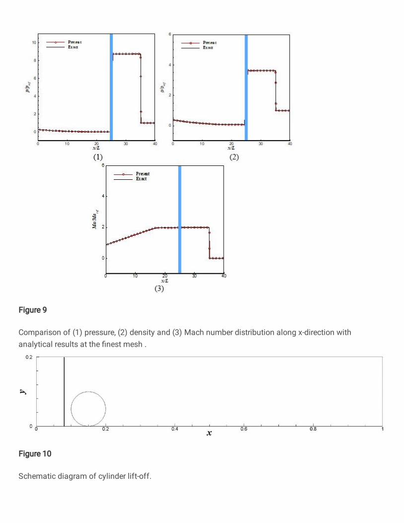
Figure 9

Comparison of (1) pressure, (2) density and (3) Mach number distribution along x-direction withanalytical results at the �nest mesh .

Figure 10

Schematic diagram of cylinder lift-off.

Figure 11

Pressure contours computed by Shyue [31] at different time: (1) t = 0.1641s , and (2) t = 0.30085s .

Figure 12

Present pressure contours ( ) at different time: (1) t = 0.1641s , and (2) t = 0.30085s