SERI/TR-215-1781 December 1982

A Beer's-Law-Based, Simple Spectral Model for Direct Normal and Diffuse Horizontal lrradiance

Richard E. Bird

Printed in the United States of America Available from:

National Technical Information Service U.S. Department of Commerce

5285 Port Royal Road Springfield, VA 22161

Price: Microfiche $3.00

Printed Copy $4.50

NOTICE

This report was prepared as an account of work sponsored by the United States Government. Neither the United States nor the United States Department of Energy , nor any of their employees, nor any of their contractors, subcontractors, or their employees, makes any warranty, express or implied, or assumes any legal liability or responsibility for the accuracy, completeness or usefulness of any information, apparatus, product or process disclosed, or represents that its use wou ld not infringe privately owned rights.

SERI/TR-215-1781 UC Categories: 59, 61, 62, 63

A Beer's-Law-Based, Simple Spectral Model for Direct Normal and Diffuse Horizontal lrradiance

Richard E. Bird

December 1982

Prepared Under Task No. 1473.00 WPA No. 424-82

Solar Energy Research Institute A Division of Midwest Research Institute

1617 Cole Boulevard Golden, Colorado 80401

Prepared for the U.S. Department of Energy Contract No. EG-77-C-01-4042

S:~l 1.1 ____________________ TR_-_17_81

PREFACE

This report documents work performed by the Solar Energy Research Institute (SERI) Renewable Resource Assessment and Instrumentation Branch for the U.S. Department of Energy under Task No. 1093.00. It presents an extremely simple solar spectral model for direct­normal and diffuse horizontal irradiance calculations. This model will make it possible for those interested in spectral data to generate their own data for research and development applications without using a large computer.

Approved for

Richard E. Bird Renewable Resource Assessment and

Instrumentation Branch

SOLAR ENERGY RESEARCH INSTITUTE

Renewable Resource Assessment and Instrumentation Branch

~ ~ µ;rf ~ J,,. 9.1. ~ Jack Stone, Acting M:6nager ~ 7'" Solar Electric Conversion Research

Division

iii

55, 1,•, ____________________ T_R_-1_1_a1

SUMMARY

OBJECTIVE

To formulate a simple spectral model for calculating solar irradiance that can be used on small computers and provide accurate results.

DISCUSSION

In the past, accurate calculations of terrestrial spectral irradiance, espe­cially the diffuse component, have necessitated the use of complex radiative transfer codes on a large main-frame computer. Such codes could thus be used by only a small group of researchers. In the work reported here, we have attempted to formulate a reasonably accurate, simple spectral model that can be applied to a broad range of atmospheric conditions.

CONCLUSIONS

We have formulated a simple spectral model that produces a spectrum between 0.3 and 4.0 µm wavelength of approximately 10 run spectral resolution. The diffuse component of the radiation obtained from this model is limited to that falling on a horizontal surface. The only inputs required for the model are turbidity coefficients, amount of water vapor, amount of ozone, solar zenith angle, surface pressure, and ground albedo.

V

55, 1,•, ___________________ T=-R--=1.!.-::1a:.:...1

LO

2.0

3.0

4.0

s.o

6.0

7.0

8.0

9.0

10.0

TABLE OP' COBTENrS

Introduction •••••••••••••••••••••••••••••••••••••••••••••••••••••••

Direct Normal Irradiance •••••••••••••••••••••••••••••••••••••••••••

Rayleigh Scattering ••••••••••••••••••••••••••••••••••••••••••••••••

Aerosol Scattering and Absorption ••••••••••••••••••••••••••••••••••

Water Vapor Absorption •••••••••••••••••••••••••••••••••••••••••••••

Ozone and Uniformly Mixed Gas Absorption •••••••••••••••••••••••••••

Diffuse Horizontal Irradiance ••••••••••••••••••••••••••••••••••••••

Comparisons with Rigorous Codes ••••••••••••••••••••••••••••••••••••

Conclusions ••••••••••••••••••••••••••••••••••••••••••••••••••••••••

References •••••••••••••••••••••••••••••••••••••••••••••••••••••••••

Appendix: Program Listing •••••••••••••••••••••••••••••••••••••••••••••••

vii

1

3

7

9

13

15

17

21

29

31

33

s:,1 ·•I ____________________ --.,TRu-----1Z-&i--i

LIST OP FIGURES

4-1 Aerosol Particle Size Distribution for Rural Aerosol Model......... 9

8-1 Comparison of SPECTRAL and BRITE Spectra for USS Atmosphere, ,: ( 0. 5) = 0. 1, ALB = 0. 0, and AM 1 • • • • • • • • • • • • • • • • • • • • • • • • • • • • • • • • • 2 2

a

8-2 Comparison of SPECTRAL and BRITE Spectra for USS Atmosphere, ,: (0.5) = 0.1, ALB= 0.0, and AM 5.6 ••••••••••••••••••••••••••••••• 22

a

8-3 Comparison of SPECTRAL and BRITE Spectra for USS Atmosphere, ~ (0.5) = 0.27, ALB= O.O, and AM 1 •••••••••••••••••••••••••••••••• 23

a

8-4 Comparison of SPECTRAL and BRITE Spectra for USS Atmosphere, ,: (0.5) ::: 0.27, ALB = O.O, and AM 2... •• •• •• •• • ••• •• ••• • • ••• •• • • ••• 23

a

8-5 Comparison of SPECTRAL and BRITE Spectra for USS Atmosphere, ,: (0.5) = 0.37, ALB= O.O, and AM 5.6 •••••••••••••••••••••••••••••• 24

a

8-6 Comparison of SPECTRAL and BRITE Spectra for USS Atmosphere, ,: ( 0 • 5) = 0 • 51, ALB = 0 • 0 , and AM 1 • • • • • • • • • • • • • • • • • • • • • • • • • • • • • • • • 2 4

a

8-7 Comparison of SPECTRAL and BRITE Spectra for USS Atmosphere, ,: (0.5) = 0.51, ALB= O.O, and AM 2 •••••••••••••••••••••••••••••••• 25

a

8-8 Comparison of SPECTRAL and BRITE Spectra for USS Atmosphere, ,: ( 0. 5) = 0. 1, ALB = 0. 2, and AM 1 • 5 • • • • • • • • • • • • • • • • • • • • • • • • • • • • • • • 2 6

a

8-9 Comparison of SPECTRAL and BRITE Spectra for USS Atmosphere, ,: (0.5) = 0.37, ALB= 0.8, and AM 1.5 •••••••••••••••••••••••••••••• 26

a

8-10 Comparison of SPECTRAL and SOLTRAN 5 Spectra for SAW Atmosphere, ,: (0.5) = 0.27, AM 1, and W = 0.42 cm •••••••••••••••••••••••••••••• 27

a

8-11 Comparison of SPECTRAL and SOLTRAN S Spectra for Tropical Atmosphere,,: (O.S) = 0.27, AM 1, and W = 4.12 cm •••••••••••••••••• 27

a

A-1 FORTRAN Program Listing for SPECTRAL ••••••••••••••••••••••••••••••• 34

ix

S:t1,., ----------------------"T=R-"""""'1 __ 78=-1

LIST OF TABLES

2-1 The Neckel and Labs Revised Extraterrestrial Spectrum and Atmospheric Absorption Coefficients at 122 Wavelengths.............. 4

4-1 Optical Parameters of the Rural Aerosol Model at

4-2

7-1

7-2

7-3

7-4

Se lee ted Wavelengths.. • • • • • • • • • • • • • • • • • • • • • • • • • • • • • • • • • • • • • • • • • • • • • • 10

Angstrom Turbidity Coefficients for Several Turbidities in the Rural Aerosol Model ••••••••••••••••••••••••••••••••••••••••••

Diffuse Correction Factor for "t (0. 5) = 0. 1 . ........................ a

Diffuse Correction Factor for "t (0.5) = 0. 2 7 . •...••••..•....•..••.•• a

Diffuse Correction Factor for,; (0.5) = 0. 3 7 . •.••••.......•..•••...• a

Diffuse Correction Factor for,; (0.5) = 0. 51 . ....................... a

xi

11

17

18

18

18

55, 1,•, _______________________ T_R_-_11_s_1

SECTION 1.0

INTRODUCTION

Solar spectral data for a wide range of atmospheric conditions at the earth's surface are required for the development of solar energy devices and perfor­mance evaluations. In the past, detailed studies have been performed using the results from rigorous radiative transfer codes (1-3]. This has seriously limited the use of accurate modeled data, because these rigorous codes are complex and require large computing capabilities. To alleviate this problem, we have been investigating methods of simplifying the rigorous codes and attempting to use a simple Beer's law approach that has met with limited pre­vious succsss [4-7].

We have determined that quite accurate results can be obtained for calcula­tions at the earth's surface with a single homogeneous layer model. This greatly reduces the computation time for a rigorous deterministic model, and we believe it is possible to produce a model that would be easy to use even with little knowledge of atmospheric physics or meteorology. Such a model would make rigorous calculations possible for a much larger group of research­ers, but it would still require substantial computer capacity. This model can be used at the surface of the atmosphere and possibly at the top, but not at p~ints between atmospheric boundaries.

We have pursued the second approach: using a Beer's law formalism based on the work of Leckner [6] and Brine and Iqbal (7). With this approach, it appeared possible to produce a simple model that could be used on microcompu­ters for surface calculations. In the sections that follow, we present a model--the result of modifications of the aforementioned models--with which we obtained good agreement with rigorous code results.

1

5 -,,~~ ,. -:· · 111.JII - ~

......

2

$:,, ,., --------------------____;;;;,TR~-_;;;;1..:......:78=-=-1

SECTION 2.0

DIRECT NORMAL IRRADIANCE

The irradiance on a surface normal to the direction of the sun at ground level for a wavelength A µ m is

le£\ = Ho\ TrA TBA To\ Tw\ TUA (2-1)

Equation 2-1 can be multiplied by cos z, where z is the solar zenith angle, to obtain the direct irradiance on a horizontal surface. The extraterrestrial spectral irradiance Ho\ at the mean solar distance based on the Neckel and Labs spectrum [8) is used here. A modified and extended version of this spec­trum ( obtained from Frohlich and Werli of the World Radiation Center, Davos, Switzerland) is the one actually used in this model. Wavelengths were selected based on measured spectra [9] at 122 wavelengths between 0.3 µm and 4.0 µm to reproduce a spectrum of approximately 10 run spectral resolution. The extraterrestrial spectrum taken from a 10-nm-resolution spectrum is given in Table 2-1, along with absorption coefficients for the 122 wavelengths.

TrA, TBA, To\, Tw\, and Tu\ are the transmittance functions for Rayleigh scat­tering, aerosol extinction, ozone absorption, water vapor absorption, and absorption by uniformly mixed gases (oxygen and carbon dioxide), respectively.

3

S::fl 1

.'

TR-1781

Table 2-1. 'l'he Neckel and Labs Revised Extraterrestrial Spectrum and Atmospheric Absorption Coefficients at 122 Vave-lengths

Wavelength Extraterrestrial

(µm) Spe2trum aWA aOA auA (W/m /µm)

0.300 535.9 0 6.69 0 0.305 558.3 0 5.50 0 0.310 622.0 0 2.10 0 0.315 692.7 0 1.35 0 0.320 715.1 0 0.800 0 0.325 832.9 0 0.380 0 0.330 961.9 0 0.160 0 0.335 931.9 0 0.095 0 0.340 900.6 0 0.040 0 0.345 911.3 0 0.019 0 0.350 975.5 0 0.007 0 0.360 975.9 0 0 0 0.370 1119.9 0 0 0 0.380 1103.8 0 0 0 0.390 1033.8 0 0 0 0.400 1479.1 0 0 0 0.410 1701.3 0 0 0 0.420 1740.4 0 0 0 0.430 1587.2 0 0 0 0.440 1837.0 0 0 0 0.450 2005.0 0 0.003 0 0.460 2043.0 0 0.006 0 0.470 1987.0 0 0.009 0 0.480 2027.0 0 0.014 0 0.490 1896.0 0 0.021 0 0.500 1909.0 0 0.030 0 0.510 1927.0 0 0.040 0 0.520 1831.0 0 0.048 0 0.530 1891.0 0 0.063 0 0.540 1898.0 0 0.075 0 0.550 1892.0 0 0.095 0 0.570 1840.0 0 0.120 0 0.593 1768.0 0.075 0.119 0 0.610 1728.0 0 0.132 0 0.630 1658.0 0 0.120 0 0.656 1524.0 0 0.065 0 0.6676 1531.0 0 0.060 0 0.690 1420.0 0.016 0.028 0.30 0.710 1399.0 o.os 0.018 0 o. 718 1374.0 1.80 0.015 0 0.7244 1373.0 1.0 0.012 0 0.740 1298.0 0.025 0.010 0 0.7525 1269.0 o.oos 0.008 0 0.7575 1245.0 0.0001 0.007 0 0.7625 1223.0 0.00001 0.006 4.0

4

s::,11•, TR-17&1

Table 2-1. 'lbe Beckel and Labs Bevised Extraterrestrial Spectrum and Atmospheric Absorption Coefficients at 122 Wave-lengths (Continued)

Wavelength Extraterrestrial

(µm) Spe~trum aw:\ ao:\ au:\ (W/m /µm)

0.7675 1205.0 0.00001 0.005 0.35 0.780 1183.0 0.0003 0 0 0.800 1148.0 0.0125 0 0 0.816 1091.0 1.45 0 0 0.8237 1062.0 2.1 0 0 0.8315 1038.0 0.155 0 0 0.840 1022.0 0.061 0 0 0.860 998.7 0.00001 0 0 0.880 947.2 0.0026 0 0 0.905 893.2 1.00 0 0 0.915 868.2 2.0 0 0 0.925 829.7 1.0 0 0 0.930 830.3 15.0 0 0 0.937 814.0 34.0 0 0 0.948 786.9 20.0 0 0 0.965 768.3 3.4 0 0 0.980 767.0 1.10 0 0 0.9935 757.6 0.1 0 0 1.04 688.1 0.00001 0 0 1.07 640.7 0.001 0 0 1.10 606.2 3.4 0 0 1.12 585.9 60.0 0 0 1.13 570.2 30.0 0 0 1.137 564.1 33.0 0 0 1.161 544.2 7.0 0 0 1.17 533.4 3.5 0 0 1.20 501.6 2.0 0 0 1.24 477.5 0.002 0 0.15 1.27 442.7 0.002 0 0.25 1.29 440.0 0.1 0 0.02 1.32 416.8 4.0 0 0.0002 1.35 391.4 200.0 0 0.00011 1.395 358.9 1000.0 0 0.00001 1.4425 327.5 100.0 0 0.29 1.4625 317.5 40.0 0 0.011 1.477 307.3 40.0 0 0.005 1.497 300.4 4.0 0 0.0006 1.520 292.8 0.16 0 0 1.539 275.5 0.002 0 0.005 1.558 272.1 0.001 0 0.13 1.578 259.3 0.0001 0 0.04 1.592 246.9 0.00001 0 0.06 1.610 244.0 0.0001 0 0.13 1.630 243.5 0.001 0 0.001 1.646 234.8 0.01 0 0.0014

5

sa,,,., TR-1781

Table 2-1. '11le Heckel and Labs Revised Extraterrestrial Spectrum and Atmospheric Absorption r.oefficients at 122 Wave-lengths (Concluded)

Wavelength Extraterrestrial

(µm) Spe~trum 8 wA ao1 auA (W/m /µm)

1.678 220.s 0.036 0 0.0001 1.740 190.8 1.1 0 0.00001 1.80 171.1 60.0 0 0.00001 1.860 144.5 600.0 0 0.0001 1.920 135.7 700.0 0 0.001 1.960 123.0 50.0 0 4.3 1.985 123.8 2.0 0 0.13 2.005 113.0 1.5 0 21.0 2.035 108.5 1.0 0 0.13 2.065 97.5 0.4 0 1.0 2.10 92.4 0.20 0 0.08 2.148 82.4 0.25 0 0.001 2.198 74.6 0.33 0 0.00038 2.270 68.3 0.02 0 0.001 2.360 63.8 4.0 0 0.0005 2.450 49.5 80.0 0 0.00015 2.5 48.5 310.0 0 0.00014 2.6 38.6 15000.0 0 0.00066 2.7 36.6 22000.0 0 100.0 2.8 32.0 8000.0 0 150.0 2.9 28.1 650.0 0 0.13 3.0 24.8 240.0 0 0.0095 3.1 22.1 230.0 0 0.001 3.2 19.6 100.0 0 0.8 3.3 17.5 120.0 0 1.9 3.4 15.7 19.5 0 1.3 3.5 14.1 3.6 0 0.075 3.6 12.7 3.1 0 0.01 3.7 11.5 2.5 0 0.00195 3.8 10.4 1.4 0 0.004 3.9 9.5 0.17 0 0.29 4.0 8.6 0.0045 0 0.025

6

sa,1 1•1 -------------------------------TR--.... l .... 18 .... l--

SECTION 3.0

RAYLEIGH SCATrEB.IRG

We began this work using the Leckner expression (6) for Rayleigh scattering transmittance, but we found that its results deviated from Pendorf' s data (10). We adapted the expression from LOWTRAN 5 (11], which agrees very closely with Pendorf. This expression is

TrA = exp{-M' /[A 4(115.6406 - l.335/A2)]} (3-1)

where M1

is the pressure-corrected air mass. The relative air mass is given by Kasten [12] as

M = [cos(Z) + 0.15(93.885 - Z)-1 •253 ]-l (3-2)

where Z is the apparent solar zenith angle. The pressure-corrected air mass is M

1 = MP/P

0, where P

0 = 1013 mb and P is the. measured surface pressure in

mb. Kasten's expression for relative air mass will be used in all calculations performed here unless otherwise noted.

Using the Rayleigh scattering theory [13], Pendorf 's data can be generated with a depolarization factor of 0.035. Young [14] concludes that the correct value should be 0.0279. Results shown later will indicate that Eq. 3-1, when it is used in conjunction with other expressions presented later, will produce data that agree very well with data from the BRITE radiative transfer code. A depolarization factor of 0.0279 was used in the BRITE code. Because of this good agreement, no adjustments have been made in Eq. 3-1 to reflect the new depolarization factor.

1

5 -~,.,:;~ =~·ll~r,I

8

sa,, , •. ______________________ TR_-_17_8_1

SECTION 4.0

AEROSOL SCATrEB.ING AND ABSORPTION

Aerosol scattering and absorption (extinction) are determined in one calcula­tion procedure in the rigorous codes using MIE scattering theory [13]. These time-conswning calculations require a knowledge of the aerosol particle size distribution and the particle complex index of refraction as a function of wavelength. The rural aerosol model [15] has been used in our rigorous calcu­lations. The aerosol size distribution for this model is shown in Fig. 4-1, and it is a bimodal, log-normal size distribution. The complex index of refraction for several wavelengths, the single scattering albedo, and the asymmetry factor for the aerosol model are presented in Table 4-1.

-E :i

......... C')

E (.)

.........

ci z ->--'iii C Cl)

0 ... G> .c E :J z

108

106

104

102

100

10-2 . . . 1Q·4 •

10·6

. . .

Rural Model

........

n 1 ( r) •

• • • • •

10-a.._.__ ________________ _

10-3 10-2 10-1 100 101 102

Radius (µm)

• The two dotted lines represent the individual log-normal distributions which combine to make up the rural model.

Figure 4-1. Aerosol Particle Size Distribution for Rural Aerosol Hodel

9

sa,11*, _______________________ ..... T-...aR_-_.,._12 ...... s~i

Table 4-1. Optical Parameters of the Bural Aerosol Model at Selected Wavelengths

A a n b n C w d

(µm) 1 2 0 <cos 9)

0.305 1.53 0.008 0.9280 0.6636 0.31 1.53 0.0072 0.9337 0.6612 0.32 1.53 0.0069 0.9356 0.6596 0.33 1.53 0.0059 0.9430 0.6581 0.35 1.53 0.0059 0.9426 0.6555 o.4o 1.53 0.0059 0.9423 o. 6511 0.45 1.53 0.0059 0.9416 0.6474 0.50 1.53 0.0059 0.9404 0.6436 o.55 1.53 0.0066 0.9333 0.6397 0.65 1.53 0.0068 0.9293 0.6352 0.75 1.527 0.00827 0.9144 0.6333 0.80 1.521 0.00989 0.9020 0.6329 0.84 1.521 0.0104 0.8932 0.6333 0.90 1.520 0.0115 0.8820 0.6323 0.95 1.520 0.0124 0.8728 0.6313 1.1 1.516 0.0147 0.8438 0.6307 1.29 1.496 0.0163 0.8178 0.6382 1.395 1.488 0.0112 0.8022 0.6421 1.52 1.478 0.0184 o.7823 0.6479 1.61 1.474 0.0173 0.7845 0.6503 1.80 1.421 0.0143 0.7835 0.6794 2.198 1.350 0.0108 o. 71

a A = wavelength. bn1 = real refractive index. cn2 = imaginary refractive index. dw

0 = single scattering albedo.

e<cos e > = asymmetry factor.

e

Leckner (6] uses the approximate formalism of Angstrom (16] to express the aerosol optical depth (turbidity) as a function of wavelength. This formalism assumes that the turbidity versus the wavelength on a log-log plot is linear. King and Herman [ 17] and our own unpublished measurements show that the tur­bidity often exhibits curvature on a log-log plot. In fact, the rural aerosol model shows curvature [15]. As a result, we have used the multiterm Angstrom formalism that follows for the turbidity TaA at wavelength A:

-a T, =~A. n

al\ n (4-1)

The turbidity coefficients ~ are directly proportional to the turbidity, and the coefficients a are relaeed to the aerosol size distribution. The slope of the line on a fog-log plot of turbidity versus wavelength is given by a. Using two a 's, a line with two straight segments can be formed to approximate a curved line. Table 4-2 presents values of ~ 1 and ~

2 for the different tur-

10

s:,11•1 ------------------------T~a~-;.._17+-1,8.,....1

bidities used in this work. The two values of a used for the rural aerosol model are a 1 = 1.0274 between 0.3 and 0.5 µm wavelength and a 2 = 1.2060 between 0.5 and 4.0 µm wavelength. A new value of ~ can be formed by

(4-2)

where ~ is the new value, ~ is old value for a given a , and ,; and ,; are the newnand old values, respegtively, of the turbidity at o.s µm waveleng~h.

The transmittance function for aerosols is then given by

~

TaA = exp(- ~ l nM) (4-3)

with the values of ~ and a changing at O. 5 µ m wavelength. n n

Table 4-2. Angstrom Turbidity Coefficients for Several Turbidities in the Rural Aerosol Model

't (0. 51,11n) ~1 ~2 a

0.1 0.0490 0.0433

0.21 0.1324 0.1170

0.37 0.1814 0.1603

0.51 0.2501 0.2210

11

S ... ,,,;,.-~ - 11! I - "-"

12

55, 1,•I ______________________ T_R_-_11.....;;.8......;...1

SECTION 5.0

WATER VAPOR. ABSORPTION

A modified version of Leckner's water vapor transmittance expression [6] was derived for this model, namely

TW\. = exp[-0.3285 a'W\.{w + (1.42 - w)0.5}M/(1.0 + 20.07awAM)0.45] , (5-1)

where awA. is the water vapor absorption coefficient at wavelength A, and w is precipifable water (in. cm) in a vertical path. See Table 2-1 for the values of a~ used here.

Unfortunately, thia work was begun by using the water vapor expression given in a preprint copy of Brine and Iqbal's paper [7] that had transposed numbers in it. The number O. 3285 in Eq. 5-1 was 0. 2385 in Leckner' s paper. We used the transposed number to derive water vapor absorption coefficients that agreed well with BRITE data for 1.42 cm of precipitable water. The error was discovered later when large differences with S0LTRAN 5 data were found for other amounts of water vapor. The transposed form of the equation provided good results for all air mass values, and it was determined there would still be problems with changing water vapor amounts in the original equation. So that new absorption coefficients would not have to be determined, the trans­posed form of the equation was retained, and a correction for water vapor amount was derived.

Note that the BRITE code derives its absorption coefficients from the 1978 Air Force Geophysics Laboratories line parameter data [_!.f J for use in its band absorption model. The data were degraded to 20 cm resolution for use in BRITE. It would be desirable to have the resolution constant in wavelength rather than wavenumber for this application, but that was beyond the scope of this work. As an alternative, we have selected wavelengths that appear to reproduce IO-nm-resolution experimental data. A few absorption coefficients have been adjusted to agree with experimental data when they varied from the results of the rigorous codes.

13

14

55:tl 1.1 ______________________ T_R_-_17_8_1

SECTION 6.0

OZONE AND URIFORMLY MIXED GAS ABSORPTION

Leckner's ozone transmittance equation [6] was used, which is

(6-1)

where a is the ozone absorption coefficient at wavelength A shown in Table 2-t 03 is the ozone amount in a vertical path (in cm), and M is the air mass expression for ozone given by Paltridge and Platt [19]. 0

M = 35.0/(1224 cos2(z) + l]o.s 0

(6-2)

The formalism of Van Heuklon [20) can be used to determine ozone amount if data are not available.

Leckner's expression for uniformly mixed gases [6] was used here:

Tw. = exp[-1.41 aci\ M' /(1 + 118.93 aUA M' )0.45] (6-3)

where at'IA is the absorption, coefficient and the gaseous amount combination shown 1ri Table 2-1, and M is the pressure-corrected air mass discussed earlier.

15

16

55, 1 .• 1 ----------------------=-=TR;.;;._-~11;..;:;s-=-1

SECTION 7.0

DIFFUSE HORIZONTAL IRllADIANCE

Historically, diffuse irradiance has been difficult to put in simple terms with any confidence, because it is much more difficult to compute rigorously than the direct component. The methods of Brine and Iqbal [ 7], which are based on the broadband methods of Davies and Hay [21], were the starting point for this work. The equation for the scattered component on a horizontal surface at wavelength A is

(7-1)

where IrA is the Rayleigh scattered irradiance on a horizontal surface at wavelength A, IBA is the aerosol scattered component on a _horizontal surface ·at wavelength A, IR'A is the ground/air reflected irradiance on a horizontal surface at wavelength A, and~ is a correction factor that is wavelength- and zenith-angle-dependent. The correction factor "'- is shown in Tables 7-1 to 7-4 for four different turbidities and seven solar zenith angles. The follow­ing equations apply:

(7-2)

I, = H cos(Z) T ,T ,T ,T ,(1-T ,) W F aA O OA UA WA rA aA O a

(7-3)

(7-4)

(7-5)

Table 7-1. Diffuse Correction Factor for "8

(0.5) = 0.1

A oo 37° 48.19° 60° 70° 75° 80°

0.30 0.75 0.75 0.76 0.85 1.20 1.30 1.4 0.35 0.99 0.98 0.99 1.01 1.08 1.17 1.4 0.40 1.1 1.11 1.11 1.12 1.20 1.27 1.52 0.45 1.04 1.06 1.06 1.06 1.11 1.16 1.34 0.50 1.08 1.06 1.05 1.04 1.09 1.11 1.23 0.55 1.04 1.02 1.00 1.00 1.04 1.04 1.13 o. 71 1.29 1.19 1.17 1.09 1.04 0.97 0.93 0.78 1.2 1.11 1.08 1.01 1.00 0.93 0.94 0.9935 1.06 0.98 0.95 0.86 0.86 0.80 0.83 2.1 0.69 0.73 0.75 0.68 0.12 0.65 0.68 4.1 0.69 0.73 0.75 0.68 o. 72 0.65 0.68

17

S5fl 1•

1

TR-1781

Table 7-2. Diffuse Correction Factor for Ta(0.5) = 0.27

A oo 37° 48.19° 60° 70° 75° 80°

0.30 0.88 0.93 1.02 1.23 2.00 4.00 6.3 0.35 1.08 1.07 1.11 1.19 1.51 1.97 3.76 0.40 1.11 1.13 1.18 1.24 1.46 1.70 2.61 0.45 1.04 1.05 1.09 1.11 1.24 1.34 1.72 a.so 1.15 1.00 1.00 0.99 1.06 1.07 1.22 0.55 1.12 0.96 0.96 0.94 0.99 0.96 1.04 o. 71 1.32 1.12 1.07 1.02 1.10 0.90 0.80 0.78 1.23 1.09 1.05 1.07 1.00 0.85 0.78 0.9935 0.98 0.94 0.91 0.83 0.90 0.79 0.74 2.1 o.69 0.68 o. 71 0.64 0.10 0.59 0.52 4.1 0.69 0.68 0.71 0.64 0.70 0.59 0.52

Table 7-3. Diffuse Correction Factor for T8(0.5) = 0.37

A oo 37° 48.19° 60° 70° 75° 80°

0.3 0.88 0.89 0.94 1.11 1.84 3.96 12.2 0.35 1.16 LOO 1.09 1.23 1.65 2.40 5.47 0.4 1.13 1.19 1.41 1.30 1.51 2.03 2.87 0.45 1.08 1.10 1.30 1.16 1.26 1.34 1.72 o.s 1.18 1.04 1.03 1.01 1.13 1.12 1.27 o.ss 1.15 1.01 0.99 0.96 1.06 1.02 1.07 0.71 1.33 1.12 1.06 1.02 1.00 0.88 0.80 0.78 1.05 1.03 0.98 0.89 0.92 0.79 0.75 0.9935 0.94 1.00 0.88 0.82 0.90 0.80 0.77 2.1 0.76 0.78 0.84 0.70 0.77 0.69 0.57 4.1 0.76 0.78 0.84 0.10 0.77 0.69 0.57

Table 7-4. Diffuse Correction Factor for T8

(0.S) = 0.51

A oo 37° 48.19° 60° 70° 75° 80°

0.3 0.88 0.99 1.02 1.22 2.26 5.17 31.3 0.35 1.08 1.11 1.28 1.27 1.80 2.76 7.48 0.40 1.06 1.09 1.29 1.12 1.36 1.67 2.78 0.45 1.01 1.03 1.20 1.00 1.11 1.20 1.57 0.5 1.21 1.06 1.01 0.99 1.04 1.02 1.17 0.55 1.20 1.02 0.97 0.95 0.97 0.92 0.98 0.71 1.21 1.09 1.04 0.95 0.94 0.82 o. 71 0.78 1.14 0.97 0.96 0.88 0.92 0.77 0.68 0.9935 0.98 0.99 0.93 0.84 0.89 o. 73 0.69 2.1 0.69 0.63 o. 71 0.73 0.81 0.72 0.78 4.1 0.69 0.63 o. 71 o. 73 0.81 o. 72 0.78

18

S:~l 1.1 ____________________ TR_-1_7~81

The albedo of the air is p , and the primes on the transmittance terms indi­s cate that they are evaluated at an air mass of 1.9. The ground albedo is

p 2

, W0

is the single scattering albedo of the aerosol, and Fa is the forward to total scattering ratio of the aerosol. F = (1 + <cos 9))0.S where <cos 9)

a is the asymmetry factor of the aerosol. Tne value of W

0 used for the rural

aerosol is O. 928, and the value of F was O. 82. Equations 7-1 to 7-5 are a

identical to those of Brine and Iqbal [7] except for the correction factor <i. An extensive attempt was made to modify Eqs. 7-2 through 7-4 so that simple equations could be used instead of the correction tables. However, all attempts to fit the equations to a set of data for several turbidities and zenith-angle combinations were unsuccessful. Even though the equations gave fairly accurate results for some conditions, it was impossible to get equa­tions of this general form to fit many conditions. In fact, the problem may be so complex that it precludes a solution involving only simple equations.

From a physics standpoint, there are several problems associated with these equations: ( 1) the cos Z terms strictly apply only to direct irradiance; (2) the transmittance terms apply to direct irradiance and are not expected to apply to scattered irradiance; and (3) W and F are wavelength-dependent, as shown in Table 7-2. Our attempts to use

0a varia\le metric minimization method

to allow the equations to seek modified forms were unsuccessful. As a result, W

0 and Fa were held constant, and the correction factors for the diffuse com­

ponents were derived at a few wavelengths. Linear interpolation was used to obtain correction factors between the tabulated wavelengths.

We must emphasize that these equations and correction factors apply only to diffuse horizontal irradiance. Normal diffuse irradiance cannot be obtained by removing the cos Z term, as we did to obtain direct normal irradiance. Our calculations show that a new set of equations and correction factors will be required for normal diffuse irradiance.

This diffuse model is only as accurate as the BRITE model. We have made some comparisons between the BRITE diffuse results and experimental data, and ini­tial indications are that the BRITE results may be slightly high for air mass values less than two. More comparisons are required to confirm this, but we feel that the BRITE diffuse component is within 15% agreement with experimen­tal data between 0.4 and 1.8 µm. The accuracy of our experimental data is in question outside this range, and is currently being improved through equipment modifications.

19

20

sa,1,•I _____________________ TR_-_11......;.s_1

SECTION 8.0

COMPARISONS WITH RIGOR.ODS CODES

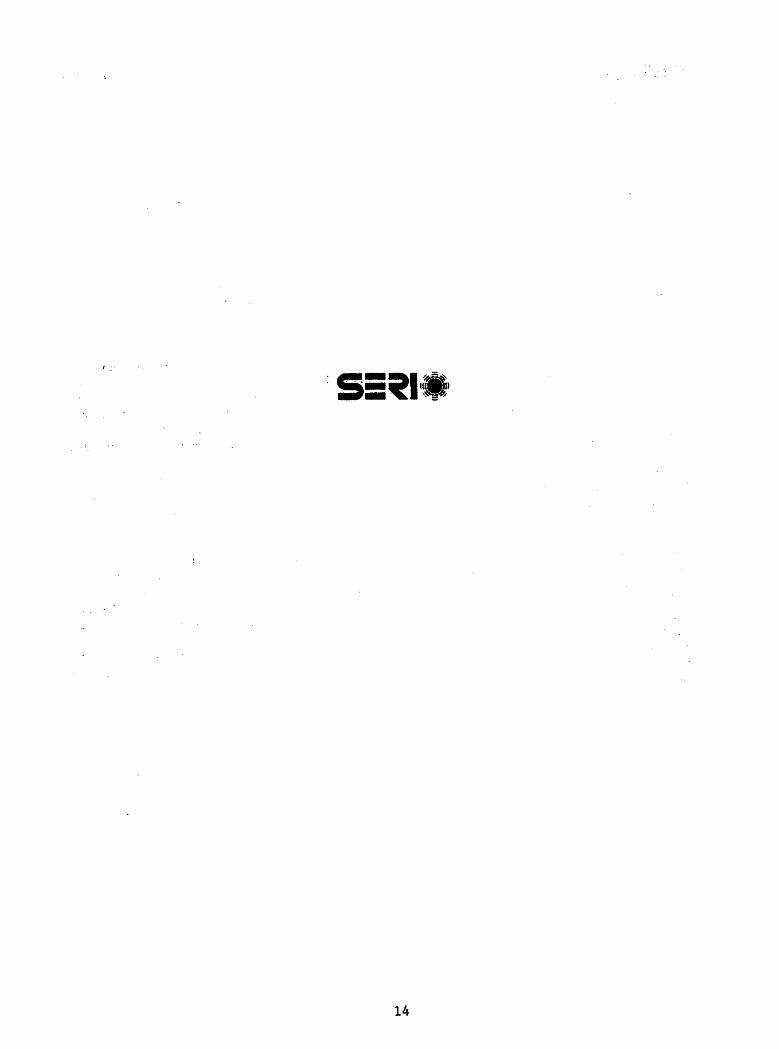
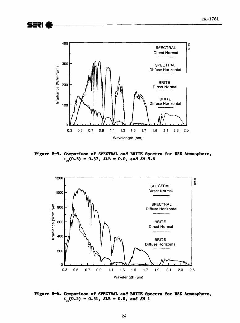
Several examples of plotted spectra that compare results from BRITE and SOLTRAN 5 with the simple model we have described will be presented here. The simple model is called SPECTRAL for identification purposes. In Figs. 8-1 through 8-7, the U.S. Standard (USS) atmospheric model [22] and the rural aerosol model [15] are used to generate plots of solar irradiance versus wave­length. Direct normal and diffuse horizontal irradiance are plotted for the BRITE and SPECTRAL models. In all of these figures, the ground albedo (ALB) is assumed to be zero, and the turbidity ['t (0.5)] and the air mass (AM) are varied. The USS atmosphere contains 1.4~ cm of precipitable water and 0.344 cm of ozone in a vertical path from sea level to 100 km altitude. In Figs. 8-1 through 8-4, a 5-nm-resolution extraterrestrial spectrum was used in BRITE and a 10-nm-resolution extraterrestrial spectrum was used in SPECTRAL, which causes the structure of the Fraunhofer lines to be slightly different. In addition, a few of the wavelengths in SPECTRAL were shifted slightly to make the results more closely resemble 10-nm-resolution experimental data that we have taken.

In Figs. 8-5 through 8-7, the resolution of the extraterrestrial spectrum and the wavelengths used are identical in both models. The turbidity in Figs. 8-1 and 8-2 is 0.1, and spectra for AM 1 and AM 5.6 are presented in that order. In Figs. 8-3 and 8-4, the turbidity is O. 27, and AM 1 and AM 2 spectra are presented. Figure 8-5 presents spectra for a turbidity of 0.37 and AM 5.6. Figures 8-6 and 8-7 are spectra for a turbidity of o. 51 and AM 1 and AM 2, respectively. These figures represent comparisons of a wide range of turbid­ity and air-mass combinations. In all cases, the direct normal component is in excellent agreement for the two models. The slight difference arising from the two models between 1.1 and 1. 3 µ m wavelength was introduced intentionally to make the SPECTRAL results look more like measured spectra. At most wave­lengths, the global horizontal spectra from the two models agree well. Occa­sionally, differences arise because of the limited number of wavelengths used in determining the tabulated correction factors.

21

TR-1781 sa,1 1•,-----------------

1600 ,n ;,; 0 0

1400 SPECTRAL Direct Normal

1200

E SPECTRAL ::::i.. t 1000 Diffuse Horizontal ........ -·-·-~ Q) 800

BRITE u C Direct Normal co "O 600 ·------t

400 BRITE Diffuse Horizontal

-----200

0 L.J...J...J......L..L~-LIL...L~C.:C:::::i:::::li.ak,Jd=~,L.L..L..1.~-A-1L....L.::L..L.oa.....L..L..L....L-1.....L..;L...L..~

0.3 0.5 0.7 0.9 1.1 1.3 1.5 1.7 1.9 2.1 2.3 2.5

Wavelength (µm)

Figure 8-1. Comparison of SPECTRAL and BRITE Spectra for USS Atmosphere, T 8 (0.5) = 0.1, ALB= 0.0, and AM 1

800 U)

SPECTRAL ~ 0 0

Direct Normal

600 SPECTRAL

E ? Diffuse Horizontal

E ·-·-........

~ BRITE 400 (I)

Direct Normal (.)

C co ·------

"O

t BRITE 200 Diffuse Horizontal

-----

0 IMl-""--l-~-J.-1--1--J~.&.....L.liC--L..J....3,~~b.l....l.t&.. .................. 1...b,L.J..JL.LJ....J....&...1-LJW....~

0.3 0.5 0.7 0.9 1.1 1.3 1.5 1.7 1.9 2.1 2.3 2.5

Wavelength (µm)

Figure 8-2. Comparison of SPECTRAL and BRITE Spectra for USS Atmosphere, T

8(0.5) a 0.1, ALB~ 0.0, and AM 5.6

22

sa,1,•1 -------------------~m&,A:.,,1-1i...,.1~a1

1400 .---------------------- .... .... 0,

SPECTRAL 8

Direct Normal

? 1000 SPECTRAL ~

ft Diffuse Horizontal E

........ 800 ~ ··-·-Q.) BRITE u C 600 Direct Normal .~ "O ct! -------.... = 400 BRITE

Diffuse Horizontal

-----200

o L.L.Jw...J.-L.L..L.J..J....L..JL..J..j,-L.L~:r:J:j~~:t::::::t::::td.w.J..J...L.....~L..J..1~~

0.3 0.5 0. 7 0.9 1.1 1.3 1.5 1. 7 1.9 2.1 2.3 2.5

Wavelength (µm)

Figure 8-3. Collparison of SPECTRAL and BllITK Spectra for USS Ataosphere, Ta(0.5) a 0.27, .ALB a o.o, and AM 1

1000 CD

SPECTRAL ; 0 0

Direct Normal

800

SPECTRAL E Diffuse Horizontal ~

i;' 600 -·-·-E

........

~ BRITE Q.) Direct Normal u C ct! 400 ------· "O ~ BRITE ....

Diffuse Horizontal

200 -----

0 ........................... ....a.....J ....... .a....L....I...-J..J.-1....L..g,s_,L..L....Cl,l~i....c:::t:::t:::::t::s~~L...d:..LJ...LJ....J...JL..L.......:::~

0.3 0.5 0.7 0.9 1.1 1.3 1.5 1.7 1.9 2.1 2.3 2.5

Wavelength (µm)

Figure 8-4. Comparison of SPECTRAL and BRITE Spectra for USS Atmosphere, Ta(0.5) m 0.21, ALB• o.o. and AM 2

23

TR-1781 s:,11•1-----------------------

400 t SPECTRAL ?

0 0

Direct Normal

300 SPECTRAL E Diffuse Horizontal ? -·-·-E

........

~ 200 BRITE

Q;) Direct Normal (.) C: -------m

"O BRITE m t Diffuse Horizontal 100 -·-·-

0 ~L...J...JL..wu...1....L.J....L.1..5...J....L..llir:!...&....L..£~..1.LJ:?::c!:!b.b.....LLI..LLL..1..,;LLL...L..Ju

0.3 0.5 0.7 0.9 1.1 1.3 1.5 1.7 1.9 2.1 2.3 2.5

Wavelength (µm)

l':l.gure 8-5. Comparison of SPECTRAL and BRITE Spectra for USS Atmosphere, Ta(0.5) = 0.37, ALB~ 0.0, and AH 5.6

1200 0 m Ol ;;

SPECTRAL 0

1000 Direct Normal

E 800 SPECTRAL

? Diffuse Horizontal E -·-·-........ $'. ; 600 BRITE (.) Direct Normal C:

.~ -------"O

~ 400 BRITE

Diffuse Horizontal -----200

OL-.L-.L.........L.....L.....L......L.~_c:.....i.----1~'-=:::c:.=:z:::::i::::::~~:..a......i...-"'-.....1.-.a:~

0.3 0.5 0. 7 0.9 1.1 1.3 1 .5 1. 7 1.9 2. 1 2.3 2.5

Wavelength (µm)

Pigure 8-6. Comparison of SPECTRAL and BRITE Spectra for USS Atmosphere, Ta(0.5) a 0.51, ALB a o.o, and AH 1

24

•- TR-1781 S5tl 1:_v ----------------

E ~ "' E .........

~ Q) 0 C:

-~ "C ca t:

400

200

SPECTRAL Direct Normal

SPECTRAL Diffuse Horizontal

BRITE Direct Normal

BRITE Diffuse Horizontal

O ~&.......JL-.JL.......JLJ.......J-.1-l~-l:~~::=c=±:~~t!.i.....J......&.....L.-i:::::U 0:3 0.5 o. 7 0.9 1.1 1.3 1.5 1.7 1.9 2.1 2.3 2.5

Wavelength (µm)

Pf.gore 8-7. r.omparlson of SPECTRAL and BRITE Spectra for USS Atmosphere, T 8 (0.S) = O.Sl, ALB a 0.0, and AH 2

Figures 8-8 and 8-9 were constructed to illustrate that SPECTRAL produces results that agree with BRITE for albedos other than zero. Figure 8-8 is for a turbidity of 0.1, AM 1.5, and an albedo of 0.2. Figure 8-9 is for a turbid­ity of 0.37, AM 1.5, and an albedo of 0.8. Both of these figures contain com­parison plots of global horizontal irradiance and diffuse horizontal irradi­ance as a function of wavelength. Results from the two models agree well. A final comparison to illustrate the agreement for different amounts of water vapor is shown in Figs. 8-10 and 8-11. The comparison is made between SPECTRAL and SOLTRAN 5 for direct normal irradiance. The Subarctic Winter (SAW) atmospheric model was used to generate Fig. 8-10, where 0.42 cm of pre­cipitable water is present. The tropical atmospheric model with 4.12 cm of precipitable water was used for Fig. 8-11. Note that the SOLTRAN 5 results were generated every 100 cm-l with 20 cm-l resolution absorption coefficients. The variable wavelength resolution and spacing causes some of the evident dif­ferences. In general, the SPECTRAL model has slightly greater attenuation in the water-vapor bands than SOLTRAN 5.

If turbidities or solar zenith angles other than those shown in Tables 7-1 through 7-4 are desired, linear interpolation can be used between the tabu­lated values. '!be model for the direct normal component appears to be appli­cable to a wide range of atmospheric parameters.

25

TR-1781 SE.fl,•,--------------------

2000,--~~~~~~~~~~~~~~~~~~~~~~~~-.~

1800

1600

E 1400

~ E 1200

~ a, 1000 (J C -~ 800 "O (ti I...

i... 600

400

200

SPECTRAL Global Horizontal

SPECTRAL Diffuse Horizontal

BRITE Global Horizontal

BRITE Diffuse Horizontal

o L....a---1.--J..-L~:bc:::z:=L.-.-J..l..r.::a...J.....L..'.~L....OCI::I::::t:::~..L....__L...a_J

"' 8

0.3 0.5 0.7 0.9 1.1 1.3 1.5 1.7 1.9 2.1 2.3 2.5 2.7 2.9

Wavelength (µm)

Figure 8-8. Comparison of SPECTRAL and BRITE Spectra for USS Atmosphere, T

8(0.5) ~ 0.1, ALB= 0.2, and AH 1.5

1800 M 00

"' 0 0

1600 SPECTRAL Global Horizontal

1400

} 1200 SPECTRAL

Diffuse Horizontal E ~ 1000

-·-·-Q) BRITE (J

800 C Global Horizontal -~ "O -------(ti

600 :: I

BRITE 400 Diffuse Horizontal

----· 200

0 L-JL.-1--1--l..-L....J.!'......a....~:::X:::~.lil!-~~~~.J.Z...;.L ..... .:C:.ta....L...1.-.L.-L...J

0.3 0.5 0.7 0.9 1.1 1.3 1.5 1.7 1.9 2.1 2.3 2.5 2.7 2.9

Wavelength (µm)

l'f.gure 8-9. Q»aparison of SPECTRAL and BUTE Spectra for USS Atmosphere, T

8(0.5) • 0.37, ALB m 0.8, and AH 1.5

26

TR-1781 S5tl 1

•1---------------

1200

- 1000 E ~

E 800 ~ Q,)

g 600 -~ "C

~ ~ 400

200

SPECTRAL Direct Normal

SOL TRAN 5 Direct Normal

0 ._... ................... ___.-.__.____._ ____________ _.__......., ___ ...__..__..__ ......... i.-.;:i-... ................. -

0.3 0.5 0.7 0.9 1.1 1.3 1.5 1.7 1.9 2.1 2.3 2.5 2.7 2.9

Wavelength (µm)

Figure 8-10. Comparison of SPECTRAL and SOLTRAN 5 Spectra for SAW Atmosphere, T

8(0.5) a 0.27, AM 1, and Wm 0.42 cm

1400

1200 SPECTRAL

Direct Normal E 1000

~ E

800 SOL TRAN 5 ....... ~ Direct Normal Q,) ------u ,I C: 600 -~ "C «l t:

400

200

0 ___ ........ __ ___. _ __.____.___._ ......... _.... ____ ......__.__ _ _._...__.,__..__........_. ...... ..__. ................. __,

0.3 0.5 0.7 0.9 1.1 1.3 1.5 1.7 1.9 2.1 2.3 2.5 2.7 2.9

Wavelength (µm)

"' co ? 0 0

.., ~ 0 0

Figure 8-11. Comparison of SPECTRAL and SOLTRAR 5 Spectra for Tropical Atmosphere, Ta(0.5) .. 0.27, AH 1, and W :a 4.12 ca

27

28

$:,11•1 ---------------------------TR.-..-_..luZJ.1S1.1...J

SECTION 9.0

CONCLUSION

A very simple model for direct normal and diffuse horizontal spectral irradi­ance has been developed, which produces results that agree well with data from rigorous codes. The simplicity of the model should make it suitable for any­one desiring spectral data, and it requires a very small computing capability. The spectrum resulting from using this model was designed to represent a 10-nm-resolution spectrum, and data are given at 122 points between O. 3 and 4.0 µm wavelength. The model is limited in the diffuse component to hori­zontal calculations only. This model is only as accurate as the BRITE and SOLTRAN 5 radiative transfer codes, which are currently believed to be ±5% on the direct normal and ±15% on the diffuse horizontal.

29

5 -.,1'"•;::;~ - IH I - ~=-"

30

sa,1,., ----------------------------IJollR_-..... 1.1..1Z8 ..... J._

SECTION 10.0

REFERENCES

1. Dave, J. V. 1978. "Extensive Data Sets of the Diffuse Radiation in Rea­listic Atmospheric Models with Aerosols and Common Absorbing Gases." Solar Energy, 21; pp. 361-369.

2. Bird, R. E. 1983. "Terrestrial Solar Spectral Modeling." Solar Cells, 7; PP• 107-118.

3. Bird, R. E.; Hulstrom, R. L. "Terrestrial Solar Spectral Data Sets." Accepted for publication by Solar Energy.

4. Moon, P. 1940. "Proposed Standard Solar Radiation Curves for Engineering Use." J. Franklin Inst., 230; pp. 583-617.

5. Thomas, A. P.; Thekaekara, M. P. 1976. "Experimental and Theoretical Studies on Solar Energy for Energy Conversion." International and U.S. Programs Solar Flux. Edited by K.W. Boer. Vol. 1; pp. 338-355.

6. Leckner, B. 1978. "The Spectral Distribution of Solar Radiation at the Earth's Surface--Elements of a Model." Solar Energy, 29; pp. 143-150.

7. Brine, D. T.; Iqbal, M. 1982. "Solar Spectral Diffuse Irradiance Under Cloudless Skies." The Renewable Challenge: Part Two. Edited by B. H. Glenn and w. A. Kolar; pp. 1271-1277.

8. Neckel, H.; Labs, D. 1981. "Improved Data of Solar Spectral Irradiance From 0.33 to 1.25 µm." Solar Phys., 74; pp. 231-249.

9. Bird, R. E.; Hulstrom, R. L.; Kliman, A. w.; Eldering, H. G. 1982. "Solar Spectral Measurements in the Terrestrial Environment." Appl. Opt., 21; PP• 1430-1436.

10. Pendorf, R. 1957. "Tables of the Refractive Index for Standard Air and the Rayleigh Scattering Coefficients." J. Opt. Soc. Am., 47; pp. 176-190.

11. Kneizys, F. X.; Shettle, E. P.; Gallery, w. o.; Chetwynd, Jr., J. H.; Abreu, L. w.; Selby, J. E. A.; Fenn, R. w.; McClatchey, R. A. 1980. Atmospheric Transmittance/Radiance: Computer Code LOWTRAN 5. Tech. Rep. AFGL-TR-80-0067. Bedford, MA: U.S. Air Force Geophysics Laboratory.

12. Kasten, F. 1966. Optical Air Mass." PP• 206-223.

"A New Table and Approximate Formula for Relative Arch. Meteorol. Geophys. Bioclimatol., Ser B14;

13. Kerker, M. 1969. ation. New York:

The Scattering of Light and Other Electromagnetic Radi­Academic Press; p. 31.

31

55, 1,•I -------------------------'T=R"---=-11....;:;s~1

14. Young, A. T. 1981. "On Rayleigh Scattering Optical Depth of the Atmo­sphere." J. Appl. Meteorology, 20; pp. 328-330.

15. Shettle, E. P.; Fenn, R. w. 1975. "Models of the Atmospheric Aerosol and Their Optical Properties." Proceedings of the Advisory Group for Aerospace Research and Development Conference No. 183, Optical Propagation in the Atmosphere; pp. 2.1-2.16. Presented at the Electromagnetic Wave Propagation Panel Symposium, Lyngby, Denmark; 27-31 October 1975.

16. Angstrom, A. 1961. "Techniques of Determining the Turbidity of the Atmo­sphere." Tellus, 13; pp. 214-221.

17. King, M. D.; Herman, B. M. 1979. "Determination of the Ground Albedo and the Index of Absorption of Atmospheric Particulates by Remote Sensing. Part I: Theory." J. of the Atmospheric Sciences, 36; pp. 163-173.

18. Rothman, L. S. 1978. Parameters Compilation."

"Update of the AFGL Atmospheric Absorption Line Appl. Opt., 17; PP• 3517-3518.

19. Paltridge, G. w.; Platt, C. M. R. 1976. Radiative Processes in Meteorol­ogy and Climatology. Elsevier, New York; P• 92.

20. Van Heuklon, T. K. 1979. "Estimating Atmospheric Ozone for Solar Radia­tion Models." Solar Energy, 22; pp. 63-68.

21. Davies, J. A.; Hay, J.E. 1980. "Calculation of Solar Radiation Incident on a Horizontal Surf ace." Proceedings, First Canadian Solar Radiation Data Workshop. Edited by J. Hay and T.K. Won. Available from: Minister of Supply and Services, Canada; P• 32.

22. Mcclatchey, R. A.; Fenn, R. W.; Selby, J.E. A.; Volz, F. E.; Garing, J. s. 1972. Optical Properties of the Atmosphere. Third Edition. Tech. Rep. AFCRL-72-0497. U.S. Air Force Cambridge Research Laboratories.

32

55, 1,•, ___________________ ____,T=R-__ 1 ___ 1a=-1

APPENDIX: PROGRAM LISTING

The FORTRAN listing of the computer program SPECTRAL, used on a CDC computer, is presented here. This program was used for sea-level calculations only, and no provision has been made to use the pressure-corrected air mass in the Rayleigh scattering and uniformly mixed gas transmittance calculations. The following parameters are defined in the program:

w BETAl

ALPHl

BETA2

ALPH2

RHO

= precipitable water (cm)

= turbidity coefficient (from 0.3 to 0.5 µm wavelength)

= a coefficient for aerosols (from 0.3 to 0.5 µm wavelength)

= turbidity coefficient (from 0.5 to 4.0 µm wavelength)

= a coefficient for aerosols from 0.5 to 4.0 µm wavelength

= ground albedo

03 = ozone amount (cm)

Z = solar zenith angle (deg)

OMEGA = aerosol single scattering albedo (0.928)

FAA = ratio of forward scattering to total scattering for aerosol (0.82)

NW = number of wavelengths used (122)

JJ = column in correction factor table to be read (depends on Z)

F(I,J) = correction factor table values

WVL = wavelength (µm)

HO = extraterrestrial irradiance at WVL (W/m2 /µm)

AW = water vapor absorption coefficient at WVL

AO = ozone absorption coefficient at WVL

AU = uniformly mixed gas optical depth at WVL

33

S::tl 1., _____________________ __;;T;.:;..:R-__;;l;;..;.7..;;;;.81;;;;....

PROGRAM SPCTRL(OUTPUT=65,TAP~6=0UTPUT,TAPE1,TAPE2~65,TAPE3=6~) DIMENSION FC7,11),WVC11) READC1,3) W,BET1,ALPH1,BET2,ALPH2 READ(l,1) RH0,03,Z,OMEGA,FAA,NW,JJ WR l Tl::: ( 6 , ;~ ) l.J , B 1::: f 1 , t~I.. PH 1 , BI:'. Ti?. , AL. P l·i ;?. , RHO , 0 3 , L. , OM E G '"' , FA A , t·H.J , J" J" DATA WV/. 30,. 35,. 4, , 45,. 5, , ~!=.:,, . !'1,, '7B,, <;>935, 2, 1, 4, 1 I AM=l , / ( COSD (Z) +. l ~:i* ( 93, EH3~i····Z) ·X·~· ( --1 . i.~~:d)) AM0=35./C1224.•C0SD<Z>•*2 + 1 .>••.5 WRITEC6,15) AM,AMO READ(;;,6) CCF<I,J>,I="l,7),J::::1,11) WIUTEC6,4) DD 14 I:::=1 ,NW READ<1,3) WVL,HO,AW,AO,AU DO 20 K=1 ,11 IFCWVL .LT. WV(K)) GO TO 2~ KK=K

20 CONTINUE 2~'; l<=l<K+l

DLTL=CWVL-WV<KK))/CWV(K)-WVCKK>> DLfF=OLrL*(F<JJ,K)-F(JJ,KK)) FACT=F(JJ,KK>+DLTF TR=EXPC-AM/(WVL**4,*<115.6406-1.335/WVL**2,))> TO=EXPC-A0•03•AMO) TW=EXP<-.3285•AW•CW+C1 ,42-W>•.5>•AM/((1 .+20.07•AW•AM>**•4~)) TU=EXPC-l.41*AU•AM/C(l.+118.Y3*AU*AM>**·4~)) IF < WVL. . GT . . 5) GU TD 1 0 TA=EXP < ·-B1:: T 1 ·X-AM·X-l~VL ·X··~ < -ALI:> 1·11 ) ) GO TO 11

10 1A=EXPC-BET2*AM•WVL••<-ALPH2)) 11 DIR=HO*TR•fO•TW•TU•fA

DRAY::::~·IO•COSD(Z)·lHO·X:TU*TW·X·TA·X-( 1, -TR )·X-, :;

DAER ::::HO ·X·Cm3D ( l) ·X· f"R·X· rCl·lHU·X- rw~- ( 1 • ··-TA) •OMEGA*FAA TRP=EXP(-1.9/(WVL**4,*(115.6406-1 .335/WVL.•*2,))) TOP=EXP<-A0*03•1.9) TWP=EXP<-.3285•AW•CW+(1,42-W)•.5>•1 ,9/((1.+20.0'l*AW*l.9)**·4~)) TUP=CXP<-1.41*AU•1.9/((1.+118.93•AU•1.9)M*,4S)) IF ( WVL. . GT, . 5 > GU TU 1 ;.:~ TAP=t:XP (····BETl·X-l .9·><-l~VL·X··X·( .. ··ALP:-11)) GD TO l ~3

12 TAP=EXPC-BET2•1 .9•WVL••<-ALPH2)) L5 1rnoA=:=: rop -x-ruP •nJP ~- < < 1 . ·- rR P > -x· r AP -x-. 5+ < 1 . -T r..i:> > *. 2~.~•DMEGA·x· rRP >

DGRD=CDIR•COSD(Z)+(DRAY+DAER>•FACT>•RHO•RHOA/(1 ,-RHO•RHOA) DIF=CDRAY+DAER)*fACT+DGRD DlOT=DIR•COSD<Z>+DIF WI~ I TE < 6 , ;-5 > WV L.. , D nn , D I I~ , I> IF ,. , ... ACT

14 WRITEC3,5) WVL,DTOT,DIR,DlF 1 FORMAf<~fl0.4,2I~> 2 FORMAT(5X,•W =•,F10.4/5X,*BET1 =•,F10.4/5X,•ALPH1=•,F10.4/

1 5X,*BET2 =•,F10,4/5X,•ALPH2=•,F10.4/5X,*RHO =•,Fl0.4/ 2 5X,•03 =•,F10.4/5X,•ZEN =•,F10.4/5X,•UMEGA=•,F10.4/ J 5X,*fA =•,F10.4/5X,•NW =•,!5/SX,•CULMN=•,I5)

3 FORMAT<~:;F10.4) 4 FORMAT(4X,•WAVLTH•,4X,*GLOBAL*,4X,*DIR~CT*,4X,*DIFFUSE*> 5 FORMAT(1X,5F10.4) 6 FORMAT<'i'F5.4)

15 FDl~MAT < 5X, -~AM STOP END

=•,F10.4/5X,*AMO =•,F10.4)

Figure A-1. FORTRAN Program Listing for SPECTRAL

34

Document Control , 1. SERI Report No.

Page SERI/TR-215-1781 , 2. NTIS Accession No.

4. Title and Subtitle

A Simple Solar Spectral Model for Direct Normal and Diffuse Horizontal Irradiance

7. Author(s)

Dick Bird 9. Performing Organization Name and Address

Solar Energy Research Institute 1617 Cole Boulevard Golden, Colorado 80401

12. Sponsoring Organization Name and Address

15. Supplementary Notes

16. Abstract (Limit: 200 words)

3. Recipient's Accession No.

5. Publication Date

December 1982 6.

8. Performing Organization Rept. No.

10. ProjecVTask/Work Unit No.

1473.00 11. Contract (C) or Grant (G) No.

(C)

(G)

13. Type of Report & Period Covered

Technical Report 14.

A spectral model for cloudless days that uses simple mathematical expressions and tabulated look-up tables to generate direct normal and diffuse horizontal irradiance is presented. The model is based on modifications to previously published simple models and comparisons with rigorous radiative transfer codes. This model is expected to be more accurate and to be applicable to a broader range of atmospheric conditions than previous simple models. The prime significance of this model is its simplicity, which allows it to be used on small desk-top computers. The spectrum produced by this model is limited to 0.3 - 4.0 µm wavelength with an approximate resolution of 10 nm.

17. Document Analysis

a. Descriptors Computerized simulation ; Diffuse solar radiation ; Direct solar radiation; Earth atmosphere; Tables

b. Identifiers/Open-Ended Terms Spectral model

c. UC Categories

59,61,62,63

18. Availability Statement National Technical Information Service

19. No. of Pages 46

U.S. Department of Commerce 5285 Port Royal Road Sorinafield- Viroinia 22161

20. Price

$4,50 Form No. 0069 (3-25-82)

*U.S. GOVERNMENT PRINTING OFFICE:1083-676-106 / 127