A Bayesian framework for functionaltime series analysis

Giovanni Petris∗

University of Arkansas

November 2013

Abstract

The paper introduces a general framework for statistical analysisof functional time series from a Bayesian perspective. The proposedapproach, based on an extension of the popular dynamic linear modelto Banach-space valued observations and states, is very flexible butalso easy to implement in many cases. For many kinds of data, suchas continuous functions, we show how the general theory of stochasticprocesses provides a convenient tool to specify priors and transitionprobabilities of the model. Finally, we show how standard Markovchain Monte Carlo methods for posterior simulation can be employedunder consistent discretizations of the data.

Keywords : Functional time series, dynamic linear model, probability on Ba-nach spaces.

1 Introduction

Time series data consisting of individual high or infinite dimensional obser-vations are becoming more and more common in many applied areas. As aconsequence there is a need to develop models and algorithms for the analysis

∗Email: gpetris@gmail.com

1

arX

iv:1

311.

0098

v2 [

stat

.ME

] 2

9 N

ov 2

013

and forecasting of this kind of data. Clearly any statistically sound modelshould account for the temporal dependence of the data, in addition to a pos-sibly complex correlation structure within the observations made at a specifictime point. Statistician have been working on methods for the analysis offunctional data for several years; early references are Ramsay and Dalzell(1991) and Grenander (1981), the books by Ramsay and Silverman (2006,2002), Ramsay et al. (2009), and Ferraty and Vieu (2006) provide good entrypoints to the recent literature. More recently, there has been an interest alsoin models and tools for time series of functional data, see for example Aueet al. (2009); Ding et al. (2009); Horvath et al. (2010); Hyndman and Shang(2009); Kargin and Onatski (2008); Shen (2009). The review papers by Masand Pumo (2010) and Hormann and Kokoszka (2012) contain up-to-date ref-erences, while the books by Bosq (2000) and Horvath and Kokoszka (2012)provide a comprehensive background. However, a fatisfactory treatment offunctional time series from a Bayesian perspective has been so far elusive.Our research aims at filling this gap, providing a flexible and easy-to-useclass of models for Bayesian analysis of functional time series.

From a methodological point of view, the main focus of the paper is theextension of the highly successful dynamic linear model to function spaces.Related references are Falb (1967) and Bensoussan (2003). Their extensions,however, are different from the one suggested in the present paper, sincethey focus on continuous-time processes and, most importantly, they do notprovide algorithms that are well-suited for practical applications.

The layout of the paper is as follows. We introduce in Section 2 thebasic notions related to Banach space-valued random variables that will beneeded for the subsequent development. The model we propose is discussedin Section 3, where also Kalman filter and smother in the infinite dimensionalsetting are discussed. Section 4 focus on a practical example in which themodel is applied to a time series of continuous functions. Concluding remarksare contained in Section 5.

2 Functional random variables

In this section we briefly introduce Banach space-valued random variablesand the extension of the notions of expectation and covariance to this type ofrandom variables. We also discuss Gaussian distributions on Banach spaces.Most of the material of this section is covered in great detail in the mono-

2

graphs by Bogachev (1998) and Da Prato and Zabczyk (1992). We considerin the following only separable Banach spaces. While this is a strong re-quirement from a theoretical perspective, it is not a serious limitation forapplications, since almost all Banach spaces of functions used in practice areseparable, the most notable exception being probably L∞, the space of es-sentially bounded (equivalence classes of) functions on a given measurablespace. The symbol B, possibly with a subscript, will be used to denote aseparable, but otherwise general, Banach space. We will use the notationL(B,B1) for the Banach space consisting of all continuos linear operatorsmapping B to B1. In the case when B1 = B we will abbreviate the notationto L(B). B∗ will denote the Banach space of all continuous linear functionalson B, i.e., B∗ = L(B,R). Recall that, for any A ∈ L(B,B1), the adjointoperator A∗ ∈ L(B∗1,B∗) is defined, for every b∗1 ∈ B∗1, to be the element ofB∗ defined as b 7→ b∗1(A(b)).

A Banach space-valued random variable X is a measurable function Xdefined on a given probability space and taking values in B

X : (Ω,F)→ (B,B),

where B denotes Borel σ-algebra of subsets of B. The separability assumptionimplies that B is also the σ-algebra generated by the continuous linear func-tionals on B, i.e., the smallest σ-algebra with respect to which all elementsof B∗ are measurable.

If X is a B-valued random variable and E(‖X‖) < ∞, then for everyf ∈ B∗ the real-valued random variable f(X) has finite expectation, sinceE(|f(X)|) ≤ ‖f‖E(‖X‖) <∞. Clearly the functional f 7→ E(f(X)) is linearin f ∈ B∗ and the previous inequality shows that it is continuous at zero,hence defining a continuous linear functional on B∗, i.e., an element of B∗∗.It can be shown that this element of B∗∗ has the form f 7→ f(µ) for a vectorµ ∈ B. We call this vector the expected value, or expectation, of X andwrite µ = E(X). The expected value can be characterized as the uniqueelement of B such that E(f(X)) = f(µ) ∀f ∈ B∗. Expected values commutewith continuous linear operators in the following sense: if A ∈ L(B,B1) andX is a B-valued random variable with expected value µ, then the B1-valuedrandom variable X1 = A(X) has expected value given by E(X1) = A(µ).

An argument along similar lines can be used to show that if E(‖X‖2) <∞, then the mapping λ : B∗ × B∗ −→ R specified by

λ(f, g) = E(f(X − µ)g(X − µ)

), f, g ∈ B∗

3

defines a bilinear function which, in turn, identifies a unique continuous lin-ear operator Λ ∈ L(B∗,B) via the identity λ(f, g) = f(Λ(g)). The operator Λis called the covariance operator, or just covariance, of X, while the bilinearfunction λ is called the covariance function of X. Covariance operator andcovariance function are two equivalent ways of providing the same informa-tion about the distribution of X. A covariance operator is symmetric andpositive, i.e., g(Λ(f)) = f(Λ(g)) and f(Λ(f)) ≥ 0 for all f, g ∈ B∗. Unlikewhat happens in Rn, where every symmetric, positive definite matrix is acovariance matrix, not all symmetric and positive elements of L(B∗,B) arevalid covariance operators. In fact, Λ ∈ L(B∗,B) is a covariance operatorif and only if there is a sequence xn in B with

∑n ‖xn‖2 < ∞ such that

Λ(f) =∑

n f(xn)xn for all f ∈ B∗.If X1 and X2 are B1- and B2-valued random variables, respectively, with

E(‖Xi‖2) < ∞, i = 1, 2, and expected values µ1 and µ2, then we can definethe covariance function between X1 and X2 to be the bilinear operator λ12 :B∗1 × B∗2 −→ R defined by

λ12(f1, f2) = E(f1(X1 − µ1)f2(X2 − µ2)

), fi ∈ B∗i , i = 1, 2.

The corresponding covariance operator Λ1,2 ∈ L(B∗2,B1) between X1 and X2

is determined by the relationship

f1(Λ12(f2)) = λ12(f1, f2), fi ∈ B∗i , i = 1, 2.

A B-valued random variable X with expected value µ and covarianceΛ has a Gaussian distribution if for every f ∈ B∗ the real-valued randomvariable f(X) has a Gaussian distribution. In this case, we write X ∼NB(µ,Λ). It is not hard to show that X has a Gaussian distribution if andonly if its characteristic functional (Fourier transform) has the form

ψ(f) = E(eif(X)

)= exp

if(µ)− 1

2λ(f, f)

, f ∈ B∗,

where λ is the covariance function associated with Λ. Using this characteri-zation, it is easy to see that, if A ∈ L(B,B1), then A(X) ∼ NB1(A(µ), AΛA∗).

Unlike what happens in the finite-dimensional case, for a general B thereare valid covariance operators that are not the covariance operator of anyB-valued Gaussian random variable.

To conclude this section, let us recall the definition of regular conditionaldistribution. Let Z be a random variable taking values in a measurable space

4

(S,S), and let G be a sub-σ-algebra of F . A function π : Ω × S :−→ R isa regular conditional distribution (r.c.d.) for Z given G if the following twoconditions hold.

1. For every ω ∈ Ω, π(ω, ·) is a probability on (S,S).

2. For every S ∈ S, π(·, S) is a version of P(Z ∈ S | G).

A standard result about r.c.d.’s is that if S is a Polish space with Borelσ-algebra S, then a r.c.d. for Z given G exists. In particular, this is thecase when S is a separable Banach space endowed with its Borel σ-algebra.For notational simplicity, in the following sections we will typically omit theexplicit dependence on ω of a regular conditional probability.

3 Functional dynamic linear model

We define in this section the functional dynamic linear model (FDLM) andwe discuss the extension of Kalman filtering and smoothing recursions, validin the finite-dimensional case, to the case of Banach space-valued states andobservations. We assume that the reader is familiar with the basic elements ofdynamic linear models (DLMs) from a Bayesian perspective in the standardcase of finite-dimensional states and observations, as found for example inWest and Harrison (1997) or Petris et al. (2009).

Let F, the observation space, and G, the state space, be separable Ba-nach spaces endowed with their Borel σ-algebras. Consider infinite sequencesY1, Y2, . . . and X0, X1, . . . of F- and G-valued random variables. We say thatthey form a state space model if Xt is a Markov chain and, for every t, theconditional distribution of Yt given all the other random variables dependson the value of Xt only. Let F ∈ L(G,F) and G ∈ L(G). An FDLM is astate space model satisfying the following distributional assumptions:

X0 ∼ NG(m0, C0

),

Xt|Xt−1 = xt−1 ∼ NG(G(xt−1),W

),

Yt|Xt = xt ∼ NF(F (xt), V

),

(1)

where m0 ∈ G, C0 and W are covariance operators on G, and V is a co-variance operator on F. The definition as well as Kalman recursions, givenbelow, can be extended in an obvious way to time-dependent operators F , G,

5

V and W ; we use the time-invariant version of the model in this paper mainlyfor notational simplicity. As for the finite dimensional DLM, quantities ofimmediate interest related to this model are the filtering and smoothing dis-tributions, that is, the conditional distribution of the state Xt given theobservations Y1:t (filtering distribution) and the conditional distribution ofXs, for s ≤ t, given Y1:t (smoothing distribution). In the finite dimensionalDLM all the conditional distributions of a set of states or future observations,given past observations, are Gaussian. This property extends to the FDLM.One practical issue that arises in the infinite dimensional model is that ob-servations, while conceptually infinite dimensional, have to be discretized atsome point, in order to allow proper data storage and processing. Clearlythis discretization leads in general to a loss of information. However, in thiscontext, one would hope that the inference based on the discretized data isalmost as good as the inference based on the complete, functional data, atleast if the discretized version of the data is still rich enough to carry most ofthe information from the complete data. In other words, one needs to showa continuity property of the inference – the filtering and smoothing distribu-tions – with respect to the discretization. If the discretization is defined ina way that is consistent with the infinite dimensional process, then one canshow that for the FDLM the continuity property mentioned above holds.

In order not to clutter the notation, we discuss the continuity of theposterior distribution with respect to a sequence of discretizations only inthe case of one functional observation Y and one functional state X. Clearly,the argument extends to the FDLM setting in a straightforward way. LetDn ∈ L(F,Rdn), n ≥ 1, be a sequence of linear, continuous operators. TheDn’s define by composition a sequence of random variables Yn = Dn(Y ),where Yn is Rdn-valued. We require that σ(Yn) ↑ σ(Y ), which formallyexpresses the fact that the information carried by the discretized versionYn approximates better and better the information carried by the completedatum Y , coinciding with it in the limit. Let πn be a r.c.d of X given Yn andπ a r.c.d. of X given Y . Then

limn→∞

πn = π almost surely,

where the limit is in the topology of weak convergence of probability mea-sures. Moreover, since all the πn are Gaussian distributions, and the classof Gaussian distributions is closed under the topology of weak convergence,one can also deduce that π is a Gaussian distribution as well.

6

An example of a sequence of discretizations of the type described aboveis the following. Consider F = C([0, 1]). For n ≥ 1 and 1 ≤ k ≤ 2n, letqn,k = k 2−n and define Dn : C([0, 1]) −→ R2n by the formula

Dn(y) =(y(qn,1), . . . , y(qn,2n)

).

Note that the same sequence of discretizing operators, evaluating a functionat the points of a sequence of finer and finer grids in [0,1], would not be welldefined if the functional datum Y were an element of L2([0, 1]), as it is oftenassumed in the FDA literature. In fact, in that case the value of the functionat any given point is not even well defined, since elements of L2([0, 1]) areequivalence classes of functions, defined up to equality almost everywhere.

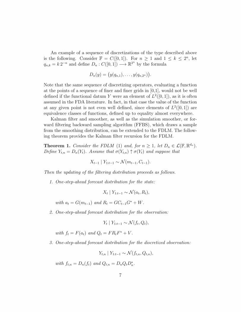
Kalman filter and smoother, as well as the simulation smoother, or for-ward filtering backward sampling algorithm (FFBS), which draws a samplefrom the smoothing distribution, can be extended to the FDLM. The follow-ing theorem provides the Kalman filter recursion for the FDLM.

Theorem 1. Consider the FDLM (1) and, for n ≥ 1, let Dn ∈ L(F,Rdn).Define Yt,n = Dn(Yt). Assume that σ(Yt,n) ↑ σ(Yt) and suppose that

Xt−1 | Y1:t−1 ∼ N (mt−1, Ct−1).

Then the updating of the filtering distribution proceeds as follows.

1. One-step-ahead forecast distribution for the state:

Xt | Y1:t−1 ∼ N (at, Rt),

with at = G(mt−1) and Rt = GCt−1G∗ +W .

2. One-step-ahead forecast distribution for the observation:

Yt | Y1:t−1 ∼ N (ft, Qt),

with ft = F (at) and Qt = FRtF∗ + V .

3. One-step-ahead forecast distribution for the discretized observation:

Yt,n | Y1:t−1 ∼ N (ft,n, Qt,n),

with ft,n = Dn(ft) and Qt,n = DnQtD∗n.

7

4. Filtering distribution at time t, given the discretized observation:

Xt | Y1:−1, Yt,n ∼ N (mt,n, Ct,n),

with mt,n = at+RtF∗D∗nQ

−1t,n(Yt,n−ft,n) and Ct,n = Rt−RtF

∗D∗nQ−1t,nDnFRt.

5. Filtering distribution at time t:

πt = limn→∞

πt,n a.s.,

where πt,n is a r.c.d. for Xt given (Y1:t−1, Yt,n) and πt is a r.c.d. for Xt

given Y1:t. Moreover, πt is a.s. a Gaussian distribution.

Proof of Theorem 1. We will first derive the joint conditional distribution of(Xt, Yt) given Y1:t−1, from which the conditional distributions in 1 and 2 willeasily follow. The dual of G× F can be identified with G∗ × F∗ noting thatthe element (x∗, y∗) ∈ G∗ × F∗ can be associated to the element of (G× F)∗

defined by˜(x∗, y∗) : (x, y) 7→ x∗(x) + y∗(y).

Moreover, every element in (G× F)∗ has that form for a unique choice of x∗

and y∗. We will make use of the following matrix notation for operators. IfA ∈ L(A,A1), B ∈ L(B,A1), C ∈ L(A,B1), and D ∈ L(B,B1), the matrix[

A BC D

]denotes the element of L(A× B,A1 × B1) defined by

A× B 3 (a, b) 7→(A(a) +B(b), C(a) +D(b)

).

It is easy to show that any element of L(A × B,A1 × B1) can be uniquelyrepresented in the matrix form written above. Let us compute the conditionalcharacteristic functional of (Xt, Yt) given Y1:t−1. For x∗ ∈ G∗ and y∗ ∈ F∗ we

8

have

ψ(x∗, y∗) = E(

exp

i(x∗(Xt) + y∗(Yt)

)|Y1:t−1

)= E

(E(

exp

i(x∗(Xt) + y∗(Yt)

)|Xt, Y1:t−1

)|Y1:t−1

)= E

(exp

ix∗(Xt) + iy∗(F (Xt))−

1

2y∗(V (y∗))

|Y1:t−1

)= E

(exp

i(x∗ + F ∗y∗

)(Xt)

|Y1:t−1

)exp

− 1

2y∗(V (y∗))

= E

(E(

exp

i(x∗ + F ∗y∗

)(Xt)

|Xt−1, Y1:t−1

)|Y1:t−1

)exp

− 1

2y∗(V (y∗))

= E

(exp

i(x∗ + F ∗y∗

)(G(Xt−1))

|Y1:t−1

)exp

− 1

2

[(x∗ + F ∗y∗)

(W (x∗ + F ∗y∗)

)+ y∗(V (y∗))

]= exp

i(x∗ + F ∗y∗

)(G(mt−1))

− 1

2

[(x∗G+ F ∗y∗G)

(Ct−1(x∗G+ F ∗y∗G)

)+ (x∗ + F ∗y∗)

(W (x∗ + F ∗y∗)

)+ y∗(V (y∗))

]= exp

i[x∗(G(mt−1)) + y∗(FG(mt−1))

]− 1

2

[x∗((GCt−1G

∗ +W )(x∗))

+ x∗((GCt−1G

∗F ∗ +WF ∗)(y∗))

+ y∗((FGCt−1G

∗ + FW )(x∗))

+ y∗((FGCt−1G

∗F ∗ + FWF ∗ + V )(y∗))]

This shows that the conditional distribution of (Xt, Yt) given Y1:t−1 is Gaus-sian with mean (at, ft) and covariance operator[

Rt RtF∗

FRt Qt

],

from which parts 1 and 2 of the theorem follow. Part 3 is an immediate

9

consequence of part 2, when one considers how Gaussian distributions trans-form under the application of a continuous linear operator. As far as part 4is concerned, if Xt were a finite dimensional random variable, then the resultwould be a straightforward application of the well-known theorem on Normalcorrelation (Lipster and Shiryayev; 1972; Barra; 1981). It is simple to verifythat the proof of that result carries over to the case where Xt is a Banachspace-valued random variable, as long as the conditioning random variableis finite dimensional. Finally, part 5 of the theorem follows from the resulton discretization of observations discussed above.

As far as the smoothing distribution is concerned, since under our mod-elling assumptions the joint distribution of (X0:t, Y1:t) is Gaussian, all itsmarginal distributions, including that of (Xs, Y1:t) are Gaussian as well. Itfollows that the conditional distribution of Xs given Y1:t is again Gaussian;that is, the smoothing distribution of Xs is Gaussian, as in the finite dimen-sional setting. In general, however, the smoothing means and covariances donot have a simple explicit form. For the purpose of applications this is nota big impediment, since the analysis is always performed on a discretizedversion of the data, to which the usual smoothing recurrence applies (Petriset al.; 2009). The inference obtained from the discretized version of theFDLM converges, as the discretization gets finer, to the inference that onewould obtain from the complete functional data, by the argument discussedbefore Theorem 1.

4 Application to C([0, 1])-valued time series

In order to define a Gaussian B-valued random variable one can rely, when Bis a Banach space of functions, on the theory of stochastic processes. WhenB = C([0, 1]), a stochastic process with continous sample paths can be inter-preted as a B-valued random variable. Let us spell out the equivalence, whichwill be used in the rest of the present section. Suppose ζ = ζt : t ∈ [0, 1] isa stochastic process with continous trajectories. Note that every ζt is a ran-dom variable, i.e., ζt = ζt(ω). Then, since the sample paths are continuous,one can define the function ζ : Ω −→ C([0, 1]) by setting

ζ(ω) : t 7→ ζt(ω), t ∈ [0, 1] and ω ∈ Ω. (2)

The following theorem shows that ζ is a C([0, 1])-valued random variableand specifies its mean and covariance function. In addition, it shows that

10

ζ has a Gaussian distribution if the process ζ does. Recall that, by Rieszrepresentation theorem, C([0, 1])∗ can be identified with the Banach spaceof all signed measures on the Borel sets of [0,1], denoted below byM([0, 1]).For η ∈M([0, 1]) and x ∈ C([0, 1]) we will use the notation

η(x) :=

∫[0,1]

x(t)η(dt).

Theorem 2. For the function defined in (2), the following hold.

1. ζ is a measurable function from (Ω,F) to the Banach space C([0, 1])endowed wih its Borel σ-algebra.

2. If, in addition, the process ζ possesses second moments, then the ex-pected value and the covariance function of ζ are given by

C([0, 1]) 3 E(ζ) : t 7→ E(ζt),

λ(η, τ) =

∫[0,1]2

γ(u, v)η(du)τ(dv), η, τ ∈M([0, 1]),

where γ(u, v) = Cov(ζu, ζv). The covariance operator of ζ is

Λ(η) =

∫[0,1]

γ(u, ·) η(du), η ∈M([0, 1]). (3)

3. If, in addition, the process ζ is Gaussian, then ζ has a Gaussian dis-tribution.

Proof. 1. See Bosq (2000), Example 1.10.

2. Let η, τ ∈M([0, 1]). In view of Jordan decomposition η = η+ − η−, sowe can assume, without real loss of generality, that η and τ are positivemeasures. By a straightforward application of Fubini’s theorem, wehave

E

(∫[0,1]

ζ(t)η(dt)

)=

∫Ω

∫[0,1]

ζt(ω)η(dt)P (dω)

=

∫[0,1]

∫Ω

ζt(ω)P (dω)η(dt)

=

∫[0,1]

E(ζt)η(dt) = η(E(ζ·)

).

11

Let m = E(ζ). Then, using Fubini’s theorem,

λ(η, τ) = E(η(ζ −m)τ(ζ −m)

)=

∫Ω

(∫[01]

(ζu(ω)−m(u)

)η(du)

)(∫[0,1]

(ζv(ω)−m(v)

)τ(dv)

)P(dω)

=

∫Ω

(∫[01]2

(ζu(ω)−m(u)

)(ζv(ω)−m(v)

)η(du)τ(dv)

)P(dω)

=

∫[01]2

(∫Ω

(ζu(ω)−m(u)

)(ζv(ω)−m(v)

)P(dω)

)η(du)τ(dv)

=

∫[01]2

γ(u, v)η(du)τ(dv).

The form of the covariance operator follows immediately from the ex-pression giving the covariance function.

3. Let η ∈ M([0, 1]) and consider the discretization operator defined forany x ∈ C([0, 1]) by

xn(t) = I0(t)x(0) +n∑

j=1

I∆n,j(t)x(j/n),

where

∆n,j =

(j − 1

n,j

n

].

It is clear that the map x 7→ xn is non-expansive, i.e., ‖yn − xn‖ ≤‖y − x‖, and therefore continuous. It follows that by applying thisoperator to ζ we obtain another C([0, 1])-valued random variable, sayζn. For any fixed ω ∈ Ω,

η(ζ(ω)

)= η(0)ζ0(ω) +

n∑j=1

η(∆n,j)ζj/n(ω).

Since the stochastic process ζ is Gaussian, the joint distribution of(ζ0, ζ1/n, . . . , ζ1) is Gaussian, hence η(ζ) is Gaussian as well. It is also

easy to show that, with probability one, ζn → ζ as n → ∞. Sinceη, as a functional on C([0, 1]), is continuous, it follows that η(ζn) →η(ζ) almost surely and, a fortiori, η(ζn)

d→ η(ζ). Since the class of

12

Gaussian distributions on R is closed with respect to the topology ofweak convergence, we conclude that η(ζ) has a Gaussian distribution.

In our numerical example below we will make extensive use of Theorem 2,using it to define Gaussian C([0, 1])-valued random variables starting fromthe Ornstein-Uhlenbeck process, having mean zero and covariance function

γ(u, v) =σ2

2βexp−β|u− v|

, (4)

where σ2 and β are positive parameters. These random variables will beused, in turn, as building blocks to set up an FDLM.

We consider a data set consisting in hourly measurements on the logscale of electricity demand, over the previous hour, collected at a distributionstation in the Northeastern region of the United States from January 2006to December 2010. We consider the data to be a discretized version of adaily functional time series. Since it is reasonable to assume that electricitydemand follows a continuous path over time, we will model the data asC([0, 1])-valued random variables. Figure 1 shows the full data set.

For scalar time series, a specific DLM that has been successfully used tomodel observations with a constant or slowly changing mean is the so-calledlocal level model. This simply consists in a random walk for a univariatestate, which is observed with noise. The model can be immediately extendedto functional data, setting F = G, F = G = 1G in (1), where, for any Banachspace B, 1B denotes the identity operator on B. We take m0 to be the zeroelement of C([0, 1]), and the covariance operators C0, W and V to be of theform (3), with γ(u, v) specified in (4). The parameters σ2 and β in (4) aredifferent for the three covariance operators and, while we fix their value whenwe define C0, so as to obtain a prior distribution for the initial state that isonly vaguely informative, we estimate the parameters of V and W , (σ2

V , βV )and (σ2

W , βW ), respectively. The inference was carried out using MCMC, sim-ulating in turn the latent states via the forward filtering backward sampling(FFBS) algorithm (Carter and Kohn; 1994; Fruwirth-Schnatter; 1994; Shep-hard; 1994), and the parameters σ2

V , βV , σ2W , βW . We coded the sampler in

the statistical programming language R (R Core Team; 2013), using also thecontributed packages zoo (Zeileis and Grothendieck; 2005) for data manipu-lation and graphing, and dlm (Petris; 2010), which contains an implementa-tion of FFBS. The prior used for the two variance parameters is an inverse

13

2006 2007 2008 2009 2010 2011

7.8

8.0

8.2

8.4

8.6

8.8

Figure 1: Electricity demand

7.8

7.9

8.0

8.1

8.2

8.3

8.4

8.5

Week of 11/23/2008

Mon Tue Wed Thu Fri Sat Sun

Figure 2: One week of electricity demand (solid line), with smoothed demand(two dash) and 90% probability bands (dashed)

14

σ2V log βV σ2

W log βW2.76 · 10−04 −2.83 2.14 · 10−04 −3.239.86 · 10−08 2.30 · 10−03 1.33 · 10−07 2.51 · 10−03

(2.70, 2.81) · 10−4 (−2.89,−2.76) (2.09, 2.20) · 10−4 (−3.30,−3.16)

Table 1: Posterior estimates, with Monte Carlo standard errors and 90%posterior probability intervals

gamma, which is conditionally conjugate for this particular model, when thelatent states are included in the simulation, while the two remaining param-eters βV and βW were updated with a random walk Metropolis-Hastings stepon the log scale. Figure 2 displays, for one particular week, the observationstogether with the smoothed states for those seven days, and 90% probabilitybands, obtained from the MCMC output. The fit is good, showing that thefunctional model, despite the small number of parameters, is flexible enoughto adapt and learn the general daily pattern of electricity demand on anygiven day.

In terms of the inference on the model parameters, Table 1 summarizesposterior estimates of the four parameters, together with MC standards errorsand 90% posterior probability intervals. MC standard errors are computedusing Sokal’s estimator (Sokal; 1989), as implemented in the R package dlm.

5 Conclusions

The model presented in the paper is an important step forward in the method-ology of analysis of functional time series. For such kind of data it providesa much more flexible setting compared to functional ARMA models (Bosq;2000; Horvath and Kokoszka; 2012). The FDLM allows to extend to thefunctional setting most of the standard structural time series models (Har-vey; 1989) that have proved extremely useful for the analysis and forecastingof finite dimensional time series. Among the advantages of the FDLM pro-posed in the paper, we note that the specification of a particular model isin most cases relatively straightforward, as illustrated in Section 4, and thepractical implementation of the posterior sampling can be done using stan-dard MCMC algorithms.

15

References

Aue, A., Gabrys, R., Horvath, L. and Kokoszka, P. (2009). Estimation ofa change-point in the mean function of functional data, Journal of Multi-variate Analysis 100: 2254–2269.

Barra, J. (1981). Mathematical Basis of Statistics, Academic Press.

Bensoussan, A. (2003). Some remarks on linear filtering theory for infinitedimensional system, in A. Rantzer and C. Byrnes (eds), Directions inMathematical System Theory and Optimization, Springer-Verlag.

Bogachev, V. (1998). Gaussian measures, American Mathematical Society.

Bosq, D. (2000). Linear processes in function spaces, Springer-Verlag, NewYork.

Carter, C. and Kohn, R. (1994). On Gibbs sampling for state space models,Biometrika 81: 541–553.

Da Prato, G. and Zabczyk, J. (1992). Stochastic equations in infinite dimen-sions, Cambridge University Press.

Ding, G., Lin, L. and Zhong, S. (2009). Functional time series predictionusing process neural networks, Chinese Physics Letters 26.

Falb, P. (1967). Infinite-dimensional filtering: the Kalman-Bucy filter inHilbert space, Information and Control 11: 102–137.

Ferraty, F. and Vieu, P. (2006). Nonparametric Functional Data Analysis,Springer-Verlag.

Fruwirth-Schnatter, S. (1994). Data augmentation and dynamic linear mod-els, Journal of Time Series Analysis 15: 183–202.

Grenander, U. (1981). Abstract Inference, Wiley.

Harvey, A. (1989). Forecasting, Structural Time Series Models and theKalman filter, Cambridge University Press, Cambridge.

Hormann, S. and Kokoszka, P. (2012). Functional time series, inT. Subba Rao, S. Subba Rao and C. Rao (eds), Handbook of Statistics,Vol. 30, Elsevier.

16

Horvath, L., Huskova, M. and Kokoszka, P. (2010). Testing the stabilityof the functional autoregressive process, Journal of Multivariate Analysis101: 352–367.

Horvath, L. and Kokoszka, P. (2012). Inference for Functional Data withApplications, Springer.

Hyndman, R. and Shang, H. (2009). Forecasting functional time series, Jour-nal of the Korean Statistical Society 38: 199–211.

Kargin, V. and Onatski, A. (2008). Curve forecasting by functional autore-gression, Journal of Multivariate Analysis 99: 2508–2526.

Lipster, R. and Shiryayev, A. (1972). Statistics of conditionally Gaussianrandom sequences, Proceedings of the Sixth Berkeley Symposium on Math-ematical Statistics and Probability, Univ. California Press, Berkeley.

Mas, A. and Pumo, B. (2010). Linear processes for functional data, in F. Fer-raty and Y. Romain (eds), The Oxford handbook of functional data, OxfordUniversity Press.

Petris, G. (2010). An R package for dynamic linear models, Journal ofStatistical Software 36(12): 1–16.URL: http://www.jstatsoft.org/v36/i12/

Petris, G., Petrone, S. and Campagnoli, P. (2009). Dynamic linear modelswith R, Springer-Verlag, New York.

R Core Team (2013). R: A Language and Environment for Statistical Com-puting, R Foundation for Statistical Computing, Vienna, Austria. ISBN3-900051-07-0.URL: http://www.R-project.org/

Ramsay, J. and Dalzell, C. (1991). Some tools for functional data analysis,Journal of the Royal Statistical Society, Series B 53: 539–572.

Ramsay, J., Hooker, G. and Graves, S. (2009). Functional Data Analysiswith R and Matlab, Springer-Verlag, New York.

Ramsay, J. and Silverman, B. (2002). Applied functional data analysis,Springer-Verlag, New York.

17

Ramsay, J. and Silverman, B. (2006). Functional Data Analysis, 2nd edn,Springer-Verlag, New York.

Shen, H. (2009). On modeling and forecasting time series of smooth curves,Technometrics 51: 227–238.

Shephard, N. (1994). Partial non-Gaussian state space models, Biometrika81: 115–131.

Sokal, A. (1989). Monte Carlo Methods in Statistical Mechanics: Foundationsand New Algorithms, Cours de Troisieme Cycle de la Physique en SuisseRomande, Lausanne.

West, M. and Harrison, J. (1997). Bayesian Forecasting and Dynamic Mod-els, 2nd edn, Springer-Verlag, New York.

Zeileis, A. and Grothendieck, G. (2005). zoo: S3 infrastructure for regularand irregular time series, Journal of Statistical Software 14(6): 1–27.URL: http://www.jstatsoft.org/v14/i06/

18