Computational Statistics and Data Analysis 55 (2011) 3320–3332

Contents lists available at ScienceDirect

Computational Statistics and Data Analysis

journal homepage: www.elsevier.com/locate/csda

A Bayesian analysis of an agricultural field trial with threespatial dimensionsMargaret Donald a,∗, Clair L. Alston a, Rick R. Young b, Kerrie L. Mengersen a

a School of Mathematical Sciences, Queensland University of Technology, GPO Box 2434, Brisbane, QLD 4001, Australiab Tamworth Agricultural Institute, Industry & Investment NSW, 4 Marsden Park Road, Calala NSW 2340, Australia

a r t i c l e i n f o

Article history:Received 31 August 2010Received in revised form 17 June 2011Accepted 17 June 2011Available online 25 June 2011

Keywords:BayesianConditional autoregressive (CAR) modelsCubic radial basesErrors-in-variablesField trialLatent variablesMarkov Chain Monte Carlo (MCMC)Markov random field (MRF)Orthogonal polynomialsSpatial autocorrelationSplinesVariance components

a b s t r a c t

Modern technology now has the ability to generate large datasets over space and time.Such data typically exhibit high autocorrelations over all dimensions. The field trialdata motivating the methods of this paper were collected to examine the behaviour oftraditional cropping and to determine a cropping systemwhich could maximise water usefor grain production while minimising leakage below the crop root zone. They consist ofmoisture measurements made at 15 depths across 3 rows and 18 columns, in the latticeframework of an agricultural field.

Bayesian conditional autoregressive (CAR) models are used to account for local sitecorrelations. Conditional autoregressive models have not been widely used in analyses ofagricultural data. This paper serves to illustrate the usefulness of these models in this field,along with the ease of implementation in WinBUGS, a freely available software package.

The innovation is the fitting of separate conditional autoregressive models for eachdepth layer, the ‘layered CAR model’, while simultaneously estimating depth profilefunctions for each site treatment. Modelling interest also lies in how best to model thetreatment effect depth profiles, and in the choice of neighbourhood structure for the spatialautocorrelation model. The favoured model fitted the treatment effects as splines overdepth, and treated depth, the basis for the regression model, as measured with error,while fitting CAR neighbourhood models by depth layer. It is hierarchical, with separateconditional autoregressive spatial variance components at each depth, and the fixed termswhich involve an errors-in-measurement model treat depth errors as interval-censoredmeasurement error. The Bayesian framework permits transparent specification and easycomparison of the various complex models compared.

© 2011 Elsevier B.V. All rights reserved.

1. Introduction

In the past 20 years, there has been a large uptake of Bayesian methods in many scientific fields, but this trend is lessprevalent in agriculture. The paper of Besag and Higdon (1999), which demonstrated Bayesian methods for an agriculturalfield trial, has been cited approximately 360 times, but of these, just 2 were published in an agricultural journal, and noneanalysed an agricultural field trial. Similarly, in a search of Web of Science on July 31, 2009, 545 papers were found whichcited Besag et al. (1991), a seminal paper for conditional autoregressive (CAR)modelling. Of these, themajority (341) relatedto health, disease or death in humans or animals, and again, none dealt with an agricultural field trial.

Almost 20 years on from Besag et al. (1991), we re-examine the advantages of the conditional autoregressive (CAR) orMarkov random field (MRF) models, described by Besag (1974) and elaborated by him and co-workers in Besag et al. (1991)

∗ Corresponding author. Tel.: +61 0 405 834 550.E-mail address:merricks.merricks@gmail.com (M. Donald).

0167-9473/$ – see front matter© 2011 Elsevier B.V. All rights reserved.doi:10.1016/j.csda.2011.06.022

M. Donald et al. / Computational Statistics and Data Analysis 55 (2011) 3320–3332 3321

and applied to field trial data in Besag et al. (1995) and Besag and Higdon (1999). Readily available software for CAR modelsallows simple specification of complex random components, and simple calculation of complex quantities based on themodel, permitting the analyst to consider many differing models.

This paper is motivated by an increasing problem in agriculture, that of understanding the impact of cropping regimeson water and, concomitantly, soil salinity. In many parts of the world the viability of rainfed grain cropping is threatenedby salination of land and water resources. Salination is caused by excessive deep drainage below the plant root zone whichmobilises sometimes vast sub-soil stores of salt deposited at the time of soil formation. Deep drainage occurs when raininfiltrates already wet soil that has insufficient capacity to store the additional water. This excess saline water may producewater logging and shallow saline water tables, or may discharge at lower points in the landscape, or into surface- or ground-waters (Broughton, 1994). When saline ground waters encroach on the crop root zone, the salt kills germinating crops orreduces yields depending on salt concentrations and rainfall (Daniells et al., 2001). The excess water is usually due to acombination of above average rainfall falling onto land farmed using long fallow cropping practices, that is, the land is keptas bare fallow for about 2/3 of the time. Although long fallow cropping usually results in good grain yields for each crop,average yields over time are generally less than yields frommore intensive, but somewhatmore risky systems. To overcomeboth the problems of excess water in the landscape under long fallow cropping, and the risk of poor crop yields due toinsufficient water supply between successive crops, when cropping is frequent, a practice of planting a crop, appropriatefor the time of year, crop health and economic considerations, in response to soil water content (opportunity or responsecropping) is being increasingly adopted by farmers. When data are collected to consider the impact of cropping regimes, asubstantive challenge of this endeavour is the description of moisture patterns over space and depth.

This paper examines a single dataset from a randomised complete block experiment, which comprises soil moisturemeasurements taken at 3 dimensions in space: row, column and depth. The presence of spatial correlation is demonstrated,and various ways are considered for modelling it. We consider several conditional autoregressive (CAR) models (Besag,1974), with a complex variance structure. We also consider an AR(1), AR(1) model such as those used by Gilmour et al.(1997) as base models, and fitted here using Markov Chain Monte Carlo Gibbs sampling, and kriging models (Cressie, 1991).

Variousmodels for the treatment effects along the depth dimension are considered, and include orthogonal polynomials,linear and cubic splines, and in conjunctionwith the splines, an errors-in-variablesmodel for depth to account for shrinkageof soils on drying, and expansion on wetting.

The interest of the final models chosen is that the data are best modelled using CAR models in two dimensions, and notthree.

2. Methods

2.1. Data

To test the efficiency of water use and the productivity of response cropping compared with long fallow systems andtraditional continuous winter cropping, a field experiment was established on a deep, well structured and well drained,non-saline, cracking clay soil (Black Vertosol) in the upper reaches of the Liverpool Plains catchment in New South Walesin south-eastern Australia. Accurate measurement of soil water content was critical to the success of this work. This wasmeasured from access tubes at measurement sites in each of 18 experimental plots over 15 equal depth increments to 3 m.The neutron scattering count (Ringrose-Voase et al., 2003) was taken at each depth in the access tube and controlled by theneutron count taken from an access tube fitted into a drum of water after each set of field measurements. The surrogatemeasurement for moisture used in the analysis here is the log transformation of the ratio of raw neutron count data to thecontrol count. Themeasurement sites were arranged as 3 rowswith 18 columns per row. Thus, the dimensions row, column,and depth are essentially orthogonal.

Nine experimental treatments consisting of three fully phased cropping systems and three types of perennial pasturewere allocated as a randomised complete block design to the 18 plots each containing 3 of the 54 measurement sites(Ringrose-Voase et al., 2003, p. 23). Treatments are described as follows.

1. Treatments 1–3. Long fallow wheat/sorghum rotation, where one wheat and one sorghum crop are grown in three yearswith an intervening 10–14month fallow period. The 3 treatments were each of 3 phases of the long fallow 3 strip system.‘Long Fallow 1’ started with wheat in the winter of 1994 followed by sorghum in summer, 1996. ‘Long Fallow 2’ startedwith sorghum in the summer of 1995, and ‘Long Fallow 3’ started with wheat in the winter of 1995.

2. Treatment 4. Continuous cropping in winter with wheat and barley grown alternately.3. Treatments 5 and 6. Response cropping, where an appropriate crop (either a winter crop or a summer crop) was planted

when the depth ofmoist soil exceeded a predetermined level. The two response cropping treatments were differentiatedby the sequence of crop types.

4. Treatments 7–9. Perennial pastures. The 3 treatments were lucerne (a deep rooted perennial forage legume with highwater use potential), lucerne grownwith awinter growing perennial grass, and amixture of winter and summer growingperennial grasses.

The data used here were from the third year of the experiment, when the treatments had bedded down and measure-ments reflected treatment effects.

3322 M. Donald et al. / Computational Statistics and Data Analysis 55 (2011) 3320–3332

Table 1Comparing spatial neighbourhood modelling. The treatment effect model is identical for all models (Orthogonal polynomial degree 8). Models have 15spatial variance components (σ 2

d ), and one homogeneous variance component (τ 2), except where otherwise stated.

Description D pD DIC 1DIC

Base model: No CAR spatial component −2609 81 −2528 –

Linear CAR (maximum 2 horiz neighbours) −3074 264 −2811 283CAR (maximum 4 horiz neighbours) −3348 358 −2990 462a

CAR (maximum 8 horiz neighbours) −3250 320 −2930 402AR(1), AR(1) −3878 923 −2956 428

CAR (maximum 4 horiz neighbours, 2 depth)b −2861 109 −2752 224CAR (maximum 4 horiz neighbours)b −2960 110 −2739 211CAR (maximum 4 horiz neighbours)c −2887 121 −2766 238

1DIC = DIC(Base Model)–DIC.a Indicates the favoured neighbourhood and random components model.b Models with 1 spatial variance and 15 non-spatial variance components.c Model with 15 spatial and 15 non-spatial variance components.

Rainfall in the 6 months preceding these moisture measurements across the entire experimental area was very high(802 mm, compared to the annual average of 684 mm). As a result, winter crops in treatments 3–7 had not substantiallydepleted the stored soil water compared with previous years. The sorghum crop in treatment 1 had recently been plantedinto a fully recharged soil profile. Plots for treatment 2 were lying fallow. In contrast, pasture plots were much drier as theywere depleted by 300–600mmcoming into thewinter. The volumetric water content calculated using the neutronmoisturemeter calibration equations from Ringrose-Voase et al. (2003) of the soils ranged from 26% under lucerne to 55% under longfallow in the surface 50 cm, illustrating the large water holding capacity of these soils.

2.1.1. Spatial correlation: existenceA well-known problem of agricultural field trials is the variability in the fertility, physical and hydraulic characteristics

of the landscape onwhich the experiment is sited. In a field trial, spatial correlation in the observations is expected since weanticipate that soil and drainage conditions of neighbouring plots are likely to be more similar than those of plots furtheraway. To reduce bias in measurements, treatments within blocks are allocated at random. However, random allocationdoes not necessarily eliminate the problem, particularly in small experiments. In addition, although the treatments forma randomised complete block treatment, there are three measurements within each treatment plot. These measurementswithin the plot are expected to be highly spatially correlated.

In preliminary analyses we fitted kriging models (Gotway and Cressie, 1990; Cressie, 1991; Banerjee et al., 2004) tothe residuals by depth layer, after fitting a saturated model of all treatments by depths (135 fixed terms). We consideredcovariograms by depth layer, and additionally allowed for anisotropy across row and column. However, neither anisotropicnor isotropic kriging models appeared satisfactory: for all depths, no covariogram showed evidence of being a function ofincreasing distance. Banerjee et al. (2004) and Stefanova et al. (2009, p. 73) indicate that such evidence is not always reliable.

Spatial correlation via a local neighbourhood definition was also considered. Moran’s I (Banerjee et al., 2004, pp. 72–73)was used to explore the spatial association of the residuals described above, using a neighbourhoodmatrix of equal weightsfor first-order neighbours in the same depth layer. Table 2 shows this as being statistically significant at the 10% level forten of the fifteen depths.

In the light of the spatial autocorrelation demonstrated by the Moran’s I analysis, a mechanism for accounting for itneeded to be included in any model fitted to the data. We adopted conditional autoregressive (CAR) models rather thankriging models, since CAR models employ sparse precision matrices (Rue and Held, 2005) rather than the dense covariancematrices used in kriging. This makes them easier to fit and more computationally efficient. Recent research (Besag andMondal, 2005; Lindgren et al., 2010) indicates that the distinction between kriging and CAR models is more apparent thanreal. (See Section 2.3 for the spatial effect modelling.)

2.2. Treatment (fixed) effects

Interest lies in describing moisture as a function of both depth and treatment. For this reason, we model depth effectsusing fixed terms in the model, rather than incorporating depth neighbours into the random CAR component of the model,except for one model (the sixth of Table 1, where we allow for residual spatial autocorrelation between adjacent depths ina three-dimensional CAR model). In this section, we describe the treatment effect modelling.

Let the sites be indexed by i = 1, . . . , 54, at depths, 20, 40, . . . , 300 (indexed by d = 1, . . . , 15). The moisture value, yi,dis modelled as nine depth functions, fj(i)(d), one for each treatment j, determined by the site index, i. These are functions ofthe depth (indexed by d). The residual from this fixed effect model is modelled as the sum of a spatial residual component,si,d, and a non-spatial residual component ϵi,d. The spatial and non-spatial residual models are described in Section 2.3.

For treatment j at site i and depth index d, the model is

yi,d = fj(i)(d) + si,d + ϵi,d,

M. Donald et al. / Computational Statistics and Data Analysis 55 (2011) 3320–3332 3323

Table 2Values of Moran’s I for each depth layer. A normalapproximation is used for the probability.

Depth Moran’s I Prob

20 −0.062 0.473040 −0.063 0.465560 0.210 0.002880 0.204 0.0037

100 0.115 0.0907120 0.125 0.0668140 0.139 0.0434160 0.107 0.1135180 −0.002 0.9199200 0.069 0.2844220 0.189 0.0068240 0.407 <0.0001260 0.242 0.0006280 0.147 0.0329300 0.176 0.0118

or alternatively,

yi,d = fj(i)(d),= Xβ, in the case of the models used,

with X being a design matrix based on the treatments j(i), and the basis functions of the depth index, d.Preliminary analyses in which possible spatial correlation was ignored showed that the data could be described in terms

of five groupings of the treatments using orthogonal polynomials of up to degree 8 for at least some of the groupings.However, we chose to fit polynomials and spline models for all 9 treatments, to permit all treatment effects to be seen,and made final comparisons across the groupings.

Soil moisture measurements were considered to be part of a continuum. To take advantage of this continuity it wasthought reasonable to approximate the treatment effects as continuous, preferably smooth, functions of depth. We fittedorthogonal polynomials, linear and cubic splines, and cubic radial bases to the depth, allowing all curves to vary across thebases by treatment.

We compared 9 treatment polynomials of degree 10, 8 and 6, with linear spline models having 3–5 internal knots, andcubic splines and cubic radial bases with 5 interior knots.

For model choice the Deviance Information Criterion (DIC) (Spiegelhalter et al., 2002) was used to compare the goodnessof fit of the various models with their differing fixed and random effects.

2.2.1. Spline and cubic radial bases modelsTreatment effects across the depths were modelled as linear splines with varying numbers of knots (from 3–5), linear

splineswith 5 knots and depth considered to bemeasuredwith error, and cubic radial basis functions (Ngo andWand, 2004)with andwithoutmeasurement error in depth.We chose to fit a measurement error model (Fuller, 1987;Wand, 2009) as analternative to the adjustment to depth used by Ringrose-Voase et al. (2003) to account for soil shrinkage/expansion underdrier/wetter conditions. While depth is measured accurately, the depth within the soil profile is not, and it is the depthwithin the soil profile which is of interest to the soil scientists. Additionally, fitting an errors-in-variables model allows thepossibility of a better fit for the spline model, and also provides a method for dealing with any residual depth correlations.For the Errors-in-variables model, see Section 2.2.2.

For the 5 knot model, 5 equally spaced internal knots were chosen at d = 3.33, 5.67, 8, 10.33 and 12.67, d = 1, . . . , 15.In this type of semi-parametric modelling, knots are typically chosen at quantiles of the data. Thus, with equally spacedobservations over depth, equally spaced knots are appropriate. The fit using the cubic radial bases did not appear to improvewith an increasing number of functions. Penalised linear and cubic splines were fitted as described by Wand (2009).

Additionally, cubic radial basis functions as defined in Ngo and Wand (2004) were fitted. These involve the inversion ofa matrix, and the use of matrix algebra. However, this matrix is fixed once the knots have been chosen. Thus, the changingbases implied by an errors-in-variables model do not require matrix inversion within an MCMC implementation.

For both the linear splines and cubic radial basis functions the Half-Cauchy distributions recommended by Marley andWand (2010) were used as prior distributions for the variance of the coefficients.

2.2.2. Errors-in-measurement modelDepth is the measured depth through the soil. However, since the soils shrink on drying and expand with moisture, the

depth index, d, does not represent the actual depth within the soil profile (Ringrose-Voase et al., 2003). Actual depth withinthe soil profile ismeasuredwith error, on any given day at any given site, because of the differentmake-up of the soil profilesand their differing moisture at any given site and depth. Hence, a measurement error model is fitted where it is assumed

3324 M. Donald et al. / Computational Statistics and Data Analysis 55 (2011) 3320–3332

that depth is measured with error in the fixed effect model for treatment, where depth is the independent variable. In thisparticular case, the errors-in-measurement model postulates that the true depth index z at any site is interval-censored.A normal interval-censored model for true depth was chosen, since the true depth z for site i at nominal depth d must liebetween the preceding true depth at nominal depth d−1 and the next true depth at nominal depth d+1. The limits of zeroand 320 (nominal depth d = 16) are commensurate with the measurements. A normal distribution, centred on d, seemedto be a reasonable description of the underlying biology.

Thus, the true depth index zi,d is interval-censored and is related to the observed depth index, d, in the following way:

zi,d ∼ N(d, σ 2z )I(zi,d−1, zi,d+1) for d = 2, 3, . . . , 14,

zi,1 ∼ N(1, σ 2z )I(0, zi,2),

zi,15 ∼ N(15, σ 2z )I(zi,14, 16),

where the prior for σ 2z is

σ 2z ∼ Half-Cauchy(1).

The choice of Half-Cauchy(1) was dictated by the need to disallow initial values of z frommoving to the extremes (0,16)and thereby removing the spline bases.

Both the spline models and the cubic radial bases model accommodate the measurement of depth with error, giving alatent true depth of z × 20 cm. Where an errors-in-variable model is used for depth, d is replaced by zi,d, the unobservedtrue depth index, and the treatment effects of the model, fj(i)(d), become fj(i)(zi,d).

2.2.3. Contrasts of interestIt was important to assess whether response cropping would use rainfall (as stored soil water) more efficiently than the

traditional practices of long fallow cropping or continuous winter cropping. Other important questions were to establishthe patterns of water use and changes in soil water profiles under response cropping compared with those under perennialpastures, which are noted for their ability to respond to rainfall and to use available soil water at most times of the year.

Thus, three contrasts were considered: (1) the difference between the traditional long fallow treatments (1, 2, 3) and theresponse cropping treatments (5, 6), (2) the difference between cropping (treatments 1–6) and pastures (7–9), and (3) thedifference between the lucerne treatments (7–8) and the perennial grass treatment (9).

The various long fallow treatments were out of phase. Thus, despite the interest being between response cropping andlong fallow cropping, all 9 depth treatment curves were fitted separately to allow any differences between them to be seen,with treatments only grouped for comparisons.

Under errors-in-measurement models of depth, treatment comparisons were made at the nominal depths.

2.3. CAR spatial models

Let the sites be indexed by i = 1, . . . , 54, at depths, 20, 40, . . . , 300 (indexed by d = 1, . . . , 15). The moisture value, yi,dis modelled as nine depth functions, fj(i)(d), one for each treatment j, determined by the site index, i. These are functions ofthe depth (indexed by d). The residual from this fixed effect model is modelled as the sum of a spatial residual component,si,d, and a non-spatial residual component ϵi,d, with ϵi,d ∼ N(0, τ 2). The spatial residual component is an average of theneighbouring spatial residuals, (Besag and Kooperberg, 1995; Besag et al., 1991). This local spatial smoothing specificationensures a global specification via Brooke’s lemma (Banerjee et al., 2004), and allows us to account for spatial similarities. Forsite i at depth d, the full model is

yi,d = fj(i)(d) + si,d + ϵi,d

where fj(i)(d) is the treatment effect for treatment j at site i and depth index d (described earlier in Section 2.2). Relabellingthe spatial residual components si,d as sm where m indexes one of the i = 1, . . . , 54 × d = 1, . . . , 15 points in the three-dimensional spatial array, the conditional probability of the spatial residual component, sm, given its neighbours, sk, is

sm|sk, k ∈ ∂m ∼ N

−k∈∂m

wmkskwm+

,σ 2

wm+

,

where ∂m is the set of indices for the neighbours of the point m, wmk is the weight of the kth neighbour of m, wm+ is thesum of the weights of the neighbours ofm, and σ 2 is a variance component for the CAR model.

However, the depth measurements differ considerably in scale from the horizontal measurements between points, andalso because treatment is modelled as a function of depth, an obvious modification of this model in a three-dimensionalcontext is to fit ‘layered’ CAR models where depth neighbours are ignored, and a point is only considered to be a neighbourif it lies in the same depth layer. This layered CAR model is described by,

si,d|sk,d, k ∈ ∂ i ∼ N

−k∈∂ i

wiksk,dwi+

,σ 2d

wi+

,

M. Donald et al. / Computational Statistics and Data Analysis 55 (2011) 3320–3332 3325

where ∂ i is the set of indices for the neighbours of site i, wik is the weight of the kth neighbour of i, wi+ is the sum of theweights of the neighbours of i. This model allows differing CAR variance components by depth. Hence the earlier σ 2 maybecome σ 2

d , with a different variance component for the CAR model at each depth, d.Finally ϵi,d, the homogeneous variance component, may also be modelled as being drawn from a set of differing variance

components, or as being drawn from a common variance component. Thus

ϵi,d ∼ N(0, τ 2), or ϵi,d ∼ N(0, τ 2d ).

Themajority of neighbourhoodmodels compared were fitted using the layered CARmodel, with varying spatial variancecomponents and a common homogeneous variance. However, one CAR model included depth neighbours and thereforecould only have a single spatial variance component (σ 2). To permit a reasonable comparison with the preceding models,we fitted the final homogeneous residual term ϵi,d with variances differing by depth, i.e., with ϵi,d ∼ N(0, τ 2

d ) for this model.A further model had 15 spatial variance components and 15 homogeneous variance components, one for each depth.

2.3.1. Neighbourhoods and weightsCAR models are based on neighbourhoods. In a three-dimensional space, there are many potential choices for the

neighbourhood of a point. A point in space could, for example, be thought of as being surrounded by 26 neighbours of a3 × 3 box, or by its first-order neighbours in both the spatial layer and over depth (6 neighbours). The major innovationof this paper is that, recognising the great differences in scale between measurements in a horizontal layer and those atdifferent depths, the neighbourhoods compared were largely within the same depth layer.

As discussed in Section 2.3, CAR models depend not only on the definition of neighbourhood, but also on the weightsgiven to neighbours, which may often be distance based. Distance weights were not used for the following reasons. Forthese data, neighbouring measurements across depth are 20 cm apart, while neighbouring measurements along rows areroughly 10 m apart when the measurement sites are in the same subplot and roughly 30 m apart when not. Along thecolumns, the distances between neighbours are approximately 20 m. Suppose that the reciprocal of the distance betweenneighbouring measurement points is used as the weight. This would mean that points within a block would weigh about3 times as much as adjacent points not in the block, thus making averaging across neighbours closer to averaging acrossa block. If depth neighbours were included, a depth neighbour would weigh 50 times more than a neighbour within theblock and 150 times more than a neighbour from a neighbouring plot. This would effectively reduce the spatial analysis to asingle dimension, depth, andmake it a depth neighbourhood analysis only. Distance weights could be discounted by raisingthe distance to a fractional power, but any discounting power is arbitrary, and would increase the number of models to bedistinguished between.

The choice of neighbourhood weights as (0, 1), i.e., a neighbour or not a neighbour, allows a simple choice of the bestadjacencymodel, independent of weights. If distance weights were to be used, it would be unclear whether it is the weightsor the adjacency definition changing the fit of the model. For example, a second-order neighbour model rejected by a (0, 1)weighting scheme, may not differ greatly from the first-order neighbour model when distance weights are used, since thedistance weights will discount the second-order neighbours. We preferred to determine appropriate neighbourhoods overwhich to average, independent of weights.

Depth neighbours were used in one CAR neighbourhoodmodel only (Table 1), as it was possible that after accounting fortreatment effects using depth (Section 2.2), neighbouring depth residuals might be correlated.

In weighting horizontal neighbours equally, the differences of scale between rows and columns are ignored. Gilmouret al. (1997) deal with this by using a basemodel with AR(1) modelling for row and column, while Besag and Higdon (1999);Besag and Mondal (2005) use differently weighted row and column CAR neighbourhood models in which the weights areestimated. Both modelling strategies recognise anisotropy, since a priori, it is unclear whether two experimental sites inadjacent rows which are physically closer will have greater spatial correlation than two sites cultivated in the same columnbut further apart. Under WinBUGS, weights may not be random quantities to be estimated, but must be fixed. Our choicewas above all to determine a suitable neighbourhood.

2.4. Choice of priors

The variances for the spatial residual components (σ 2d ) were given a common inverse gamma prior, and the non-spatial

variance component (τ 2) an inverse gamma prior. Thus,

1/σ 2d ∼ Gamma(a1, b1),

1/τ 2∼ Gamma(a2, b2), where,

al ∼ Gamma(0.1, 0.1),bl ∼ Gamma(0.1, 0.1), l = 1, 2.

For the splines and cubic radial basis functions, the coefficients of fixed terms were assigned the prior N(0, σ 2u ), with

σ 2u having a Half-Cauchy(25) prior. The latent depth variable, z, was assigned a prior of N(0, σ 2

z ), with σ 2z having a Half-

Cauchy(1) prior. These Half-Cauchy choices are not restrictive, since the median of the Half-Cauchy(1) is 1, the mode is 0,and the mid 90% of the distribution lies within (0.08, 12.7), while for Half-Cauchy(25), the mid 90% lies between (1.97, 318).

3326 M. Donald et al. / Computational Statistics and Data Analysis 55 (2011) 3320–3332

Table 3Comparing fixed effect modelling. Random components for all models are given by 4 neighbour CAR with 15 depth variances (σ 2

d ), and one homogeneousvariance component (τ 2).

Deg/Knots No. terms Type D pD DIC 1DIC

135 Saturated model (9 × 15 terms) −3127 809 −2319 –

6 63 Orthogonal poly −3267 297 −2970 6518 81 −3348 358 −2990 671a

10 99 −3338 371 −2967 648

4 54 Linear spline −3241 318 −2923 6044 54 (+error in depth) −3370 369 −3002 683a

5 63 (+error in depth) −3372 372 −3000 681a

5 81 Cubic radial bases −3281 327 −2954 6355 81 (+error in depth) −3384 368 −3013 694a

5 81 Cubic spline −3026 257 −2769 450

No. Terms is the number of fitted fixed effect terms.pD, DIC given for the moisture value to allow comparison.1DIC: DIC (saturated model)−DIC.

a Indicates the best fixed effect model of its type.

The coefficients of the orthogonal polynomials were assigned priors of N(0, 3.3). This choice was influenced by thenumber of fixed terms. With large numbers of terms, it was important to keep their sum within numeric computing rangeduring the burn-in. Given that their sum lay between −0.8 and −0.2, this prior did not seem too restrictive.

Similar considerations applied to the choice of Gamma (0.1, 0.1) for the hyperpriors for the parameters of the inversegamma distributions from which the variances for the spatial and non-spatial random components were drawn; adistribution with a mean of 1 and a variance of 10 (and mid 90% in (0,10)) seemed reasonable for these hyperpriors.

2.5. Model comparisons

In choosing a CAR and random effect model, we need to keep the fixed part constant while comparing neighbourhoodchoices and random effect models. Historically we had established that an 8 degree polynomial adequately described thefixed part. Hence, thiswas kept constant in choosing an appropriate randomeffects andCARmodel. Similarly,when choosingthe fixed part of the model, the random effects and neighbourhood models were kept constant, and here, on the basis ofTable 1, the layered CARmodel with its first-order neighbours from the same layer, the 15 spatial variance components andthe single homogeneous variance component was kept constant while varying the fixedmodels. Choices of model are madeusing the Deviance Information Criterion (DIC) (Spiegelhalter et al., 2002), available in WinBUGS.

It may be asked why we do not use Bayes factors or consider marginal likelihoods for model comparison. However, asHan and Carlin (2001) and Chen and Wang (2011) comment, Bayes factors are difficult to calculate in hierarchical models.Certainly, it would not have been feasible within the modelling framework to jointly model competing models. Havingcomputed all models separately, we do have the mean deviance for all models, which is an integral of the deviance and thusa check of the marginal likelihoods. Li et al. (2011) point out that the DIC select(s) the better predicting model, while theBayes factor chooses a better fitting model. In Tables 1 and 3, the average deviance, D, is also given. Our view is that modelchoice is better made with a criterion which penalises for the number of parameters in the model.

2.6. Implementation details

Initially, treatment effects were expressed in terms of design matrices, X, andMCMC iterations estimating the treatmenteffects iterated over all 810 observations. However, withinWinBUGS, it is more useful to think of the fittedmodels as fittinga value for each of nine treatments at each of 15 depths (135 estimates), and using indices to assign this fitted value to eachof the 6 site observations for a treatment. This change speeds convergence and reduces memory requirements.

Neighbourhood matrices, orthogonal polynomials, and the inverse matrices required by the cubic radial bases werecalculated outside WinBUGS and formed part of the data description. Spline bases were calculated in WinBUGS, which isnecessary when the errors-in-measurement model for depth was used, as the bases change with each change in the latentdepth variables.

All models were run as scripts, with at least a 60,000 iterations for burn-in (140,000 for errors-in-variables models) with200,000 iterations in all for the more complex models. Models were set up with two chains and Gelman–Rubin statisticschecked.

3. Results

3.1. Assessing presence of spatial correlation

The presence of spatial correlation was demonstrated by Moran’s I (Banerjee et al., 2004). Table 2 shows this statistic asbeing statistically significant at the 10% level for ten of the fifteen depths. The pattern of significance was also reflected in

M. Donald et al. / Computational Statistics and Data Analysis 55 (2011) 3320–3332 3327

the significance of the ratio of spatial variance to non-spatial variance differing from 1, with lower variability being shownat the central depths.

3.2. Determining neighbourhoods and random components

Table 1 compares several models with differing neighbourhood structures, and in some cases, differing randomcomponents. In this table allmodels have the same fixed design,with orthogonal polynomials of degree 8 for each treatment.The base model against which the other models of this table are compared has the same fixed design, no spatial randomeffects and a single homogeneous error. This 8 degree polynomial model was used because it had been shown to adequatelymodel the treatments as a function of depth when using a single pooled error, and examination of the residuals alongthe depth dimension had demonstrated that the model was not inducing autocorrelated residuals by depth. Models arecompared using the effective number of parameters (pD) and Deviance Information Criterion (DIC). The essential set ofcomparisons is used to determine an appropriate neighbourhood, andmost models in this table have a single homogeneousvariance component (τ 2), and 15 spatial variance components (σ 2

d ). Three additional models are considered, one of whichincludes depth neighbours andwhich thereforemust be fittedwith a single spatial variance. Thismodel has 15homogeneousvariance components (τ 2

d ). The second additional model also has 15 homogeneous variance components (τ 2d ), and although

it uses a layered 4 neighbourhood CAR model, the CAR variances at each depth are the same (σ 2). The final model has 15spatial variance components and 15 homogeneous random variance components and the same layered 4 neighbour CARstructure. The major group of comparisons is between models having the same variance structure: a random componentstructure of 15 spatial random components (σ 2

d ) and a common homogeneous variance (τ 2). Table 1 consists of models withthe following variance and CAR structures:1. The base model, with one common pooled variance for error across all sites and depths;2. CAR model with a maximum of two neighbours per site (along the row), 15 spatial variances, one for each depth, and a

single homogeneous error variance;3. CAR model with a maximum of four neighbours per site (directly adjacent in row and column), 15 spatial variances, one

for each depth, and a single homogeneous error variance;4. CAR model with a maximum of eight neighbours per site (includes diagonally adjacent sites), 15 spatial variances, one

for each depth, and a single homogeneous error variance;5. AR(1), AR(1) model (Gilmour et al., 1997), with a different autocorrelation components for each depth layer, along the

rows, and a common AR(1) component across the rows;

Table 1 also shows a further set of comparisons which allow the determination of the random component structure, andalso determine whether depth neighbours should be fitted within the CAR modelling offered under WinBUGS.1. CAR model with a maximum of 6 neighbours per site (2 of which are depth neighbours), one spatial variance, and 15

homogeneous error variances, one for each depth;2. CAR model with a maximum of 4 neighbours per site, one spatial variance, and 15 homogeneous error variances, one for

each depth;3. CAR model with a maximum of 4 neighbours per site, 15 spatial variance components, and 15 homogeneous error

variances, one for each depth.

Using the DIC criterion, the preferred model is that having a maximum of 4 neighbours in the same layer, with the 15differing spatial variances. Including depth neighbours with the one spatial variance component and the 15 non-spatialvariance components gave a poorer model fit than the 4 neighbour model with the same random component structure.Somewhat surprisingly, the 30 variance component model was less satisfactory than either of the models with the samefirst-order neighbourhood model, and 16 variance components

In Table 3 we examine various fixed effect models while using a common random component specification. All modelsin this table use a homogeneous random component, and a CAR specification with a maximum of 4 first-order neighboursin the same depth layer, and the CAR model for each depth having a differing spatial variance.1. The saturated model with 9 treatments × 15 depth terms;2. Three orthogonal polynomial models of (a) degree 6, (b) degree 8, and (c) degree 10;3. Three linear spline models with (a) 4 internal knots, (b) 4 internal knots, and the assumption of errors in the depth

measurement, and (c) 5 internal knots, and the assumption of errors in the depth measurement;4. Two cubic radial basesmodelswith 5 internal knots and (a) no assumption of error in the depthmeasurement, and (b) the

assumption of errors in the depth measurement;5. Cubic spline with 5 internal knots.

The three polynomial models were fitted to choose a good base model to allow comparison of the CARmodels, and showthat the choice of an 8 degree polynomial model was a reasonable choice for the comparisons of Table 1.

The poor fit of the saturated model (9 × 15 terms) reflects the biology of the system. Treatments become increasinglyirrelevant with depth, with the roots of each crop becoming unable to access moisture at the deeper depths. When theerrors-in-variables model is not fitted, the best model is that using orthogonal polynomials of degree 8, and the best modelof the various spline models that using cubic radial bases.

3328 M. Donald et al. / Computational Statistics and Data Analysis 55 (2011) 3320–3332

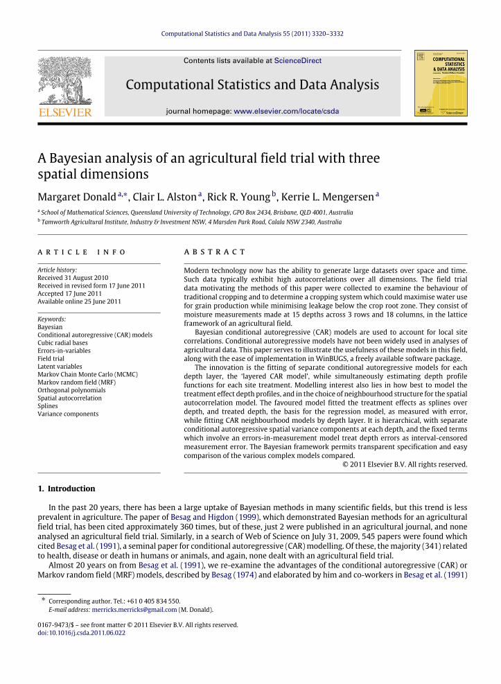
Fig. 1. 95% credible intervals for the contrast differences based on the cubic radial bases model with errors-in-measurement (graphed where the 95% CIdid not cover zero). The lines with the widest tops and tails show ‘‘Long Fallow—Response Cropping’’, with the thinnest ‘‘Lucerne—Native Pastures’’, andthose with medium width ‘‘Crop—Pasture’’.

The linear spline models with four and five knots and errors-in-measurement for depth, which are roughly equivalent,provide a better fit than the simple linear spline model.

The cubic radial bases model with the errors-in-measurement component provides the best of the spline basis fits. Notsurprisingly, the estimated number of parameters for all three errors-in-variables models is almost identical.

Of all the models, an errors-in-measurement model is preferred since this matches the known occurrence of soilshrinkage and expansion. The estimated differences between true depth and nominal depth were almost the same for boththe linear spline model and the cubic radial bases model. However, the linear spline models offer an advantage in that theypermit estimation of the slopes of the line segments and thus the possibility of determining when and where moisture isincreasing or decreasing.

Contrasts of interest were monitored at each depth. For the models without errors-in-measurement, the contrasts were,as expected, sharper than those for the models with measurement error. However, the patterns were largely the same.The major differences established between treatment groupings are those for cropping versus pasture and for lucerneversus the perennial grasses, with cropping giving the higher moisture values, perennial grasses the next highest values,and lucernes giving the lowest moisture values. The differences are most marked at the shallower depths. The hoped-fordifference between response cropping and long fallowing was observed at the intermediate depths (from 160–200 cm, forthe polynomial model, and from 180 cm–200 cm for the errors-in-variables models). See Fig. 1.

As expected, all fixed effect curves from the various fixed effectmodelswith the 4 neighbour hierarchical CARmodel havewider credible intervals than those for the correspondingmodelswith no spatial correlation taken into account (not shown).The CAR analysis is more realistic in that spatial correlation has been accounted for.

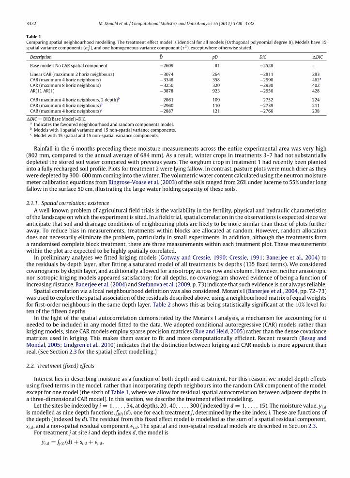
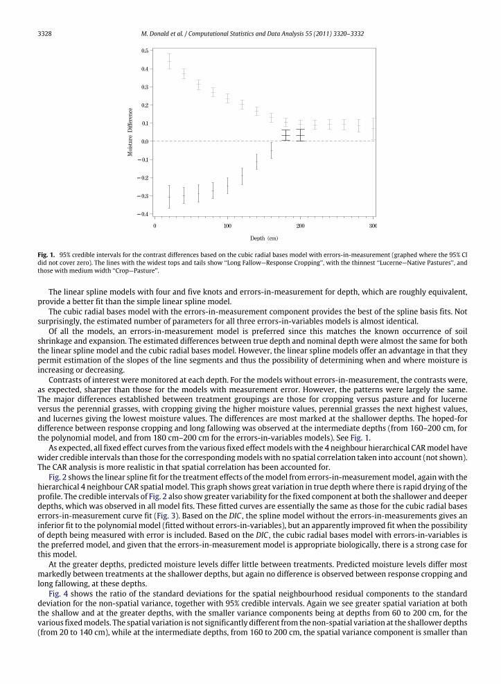
Fig. 2 shows the linear spline fit for the treatment effects of themodel from errors-in-measurementmodel, againwith thehierarchical 4 neighbour CAR spatial model. This graph shows great variation in true depthwhere there is rapid drying of theprofile. The credible intervals of Fig. 2 also show greater variability for the fixed component at both the shallower and deeperdepths, which was observed in all model fits. These fitted curves are essentially the same as those for the cubic radial baseserrors-in-measurement curve fit (Fig. 3). Based on the DIC , the spline model without the errors-in-measurements gives aninferior fit to the polynomial model (fitted without errors-in-variables), but an apparently improved fit when the possibilityof depth being measured with error is included. Based on the DIC , the cubic radial bases model with errors-in-variables isthe preferred model, and given that the errors-in-measurement model is appropriate biologically, there is a strong case forthis model.

At the greater depths, predicted moisture levels differ little between treatments. Predicted moisture levels differ mostmarkedly between treatments at the shallower depths, but again no difference is observed between response cropping andlong fallowing, at these depths.

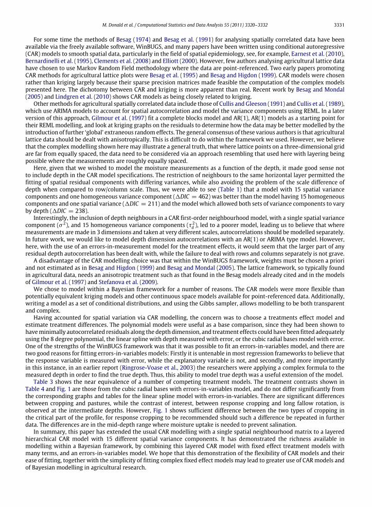
Fig. 4 shows the ratio of the standard deviations for the spatial neighbourhood residual components to the standarddeviation for the non-spatial variance, together with 95% credible intervals. Again we see greater spatial variation at boththe shallow and at the greater depths, with the smaller variance components being at depths from 60 to 200 cm, for thevarious fixedmodels. The spatial variation is not significantly different from thenon-spatial variation at the shallower depths(from 20 to 140 cm), while at the intermediate depths, from 160 to 200 cm, the spatial variance component is smaller than

M. Donald et al. / Computational Statistics and Data Analysis 55 (2011) 3320–3332 3329

Fig. 2. Fixed effect curves for errors-in-variables model: Linear spline treatment effects and 95% credible intervals, CARmodel, sites 1–54. The true depthsare those implied by the errors-in-measurement model. For each treatment there are 6 sites, each with the same treatment curve.

Fig. 3. Fixed effect curves for errors-in-variables model: cubic radial bases model showing estimates at the nominal depth. Depth has been jittered toallow credible intervals to be seen.

the non-spatial variance component, with the spatial variation being larger than the non-spatial variation at the greaterdepths (from 240 to 300 cm). This aspect of the spatial variation is consistent over the 2, 4 and 8 neighbour CARmodels, andover the spline basis and orthogonal polynomials. Perhaps surprisingly, the 7th model of Table 1, with one spatial variancecomponent and 15 non-spatial variances, is not competitive with the model in which the differing variation at the differentdepths is accounted for by 15 spatial variances (the 3rd model of the table).

Table 4 gives the contrasts between treatment types at various depths under the errors-in-variables cubic radial basesmodel. The contrasts are more tightly estimated under the model without errors-in-measurement of depth. However, thesignificant contrasts closely parallel each other. The contrasts are shown in Fig. 1.

4. Discussion

In this paper, there were two critical issues: (1) to find an appropriate way of dealing with spatial correlation, and (2) tofind an appropriatemodel for the treatment effects. Having accomplished these two goals, it then becomes possible tomakeinferences for the questions asked by the scientists.

3330 M. Donald et al. / Computational Statistics and Data Analysis 55 (2011) 3320–3332

Fig. 4. 95% CI for the ratio of square root of the spatial variance to that of the non-spatial variance at the fifteen depths: cubic radial bases model witherrors-in-measurement for depth.

Table 4Contrasts at nominal depths: Cubic radial bases model where depth is measured with error.

Contrast Depth Est 95%CI Prob

Long Fallow v Opportunity cropping 180 0.033 (0.004, 0.063) 0.0246200 0.033 (0.002, 0.066) 0.0357

Crop v pasture 20 0.440 (0.401, 0.484) <0.000140 0.372 (0.346, 0.399) <0.000160 0.314 (0.286, 0.340) <0.000180 0.270 (0.244, 0.294) <0.0001

100 0.236 (0.212, 0.261) <0.0001120 0.202 (0.178, 0.228) <0.0001140 0.164 (0.142, 0.188) <0.0001160 0.130 (0.106, 0.154) <0.0001180 0.106 (0.082, 0.129) <0.0001200 0.093 (0.069, 0.118) <0.0001220 0.090 (0.065, 0.116) <0.0001240 0.092 (0.065, 0.120) <0.0001260 0.092 (0.062, 0.122) <0.0001280 0.085 (0.050, 0.119) <0.0001300 0.071 (0.009, 0.127) 0.0279

Lucernes v native pasture 20 −0.305 (−0.369, −0.245) <0.000140 −0.301 (−0.343, −0.254) <0.000160 −0.290 (−0.333, −0.239) <0.000180 −0.273 (−0.316, −0.228) <0.0001

100 −0.243 (−0.290, −0.202) <0.0001120 −0.188 (−0.237, −0.146) <0.0001140 −0.115 (−0.155, −0.072) <0.0001160 −0.054 (−0.092, −0.006) 0.0322

Only contrasts with CIs not containing zero shown.

The primary difficulty was the determination of the spatial model. Given that the data are point-referenced, an obviouschoice of spatial model was a kriging model, such as that of Gotway and Cressie (1990). However, the large number of termsin the fixed part of the model made such an approach impossible in the MCMC framework used. Additionally, includingdepth in the calculation of distance, would have meant greater difficulties in disentangling treatment effects over depthfrom spatial modelling considerations. Software such as SAS PROCMIXED (SAS Institute, 2004) offers the possibility of bothkriging and the various correlation model structures of Gilmour et al. (1997) within a REML or ML framework, but when amodel is poorly specified or very complex, PROC MIXED can be difficult to use, and neither SAS nor the package of Gilmouret al. (2005) is freely available. We had hoped to show that the CAR models used were comparable to the AR(1), AR(1) basismodels of Gilmour et al. (1997) and Stefanova et al. (2009). These were unable to be fitted with the desired complexity, butshow comparability with the best CAR models of Table 1 (1DIC = 428).

M. Donald et al. / Computational Statistics and Data Analysis 55 (2011) 3320–3332 3331

For some time the methods of Besag (1974) and Besag et al. (1991) for analysing spatially correlated data have beenavailable via the freely available software, WinBUGS, and many papers have been written using conditional autoregressive(CAR) models to smooth spatial data, particularly in the field of spatial epidemiology, see, for example, Earnest et al. (2010),Bernardinelli et al. (1995), Clements et al. (2008) and Elliott (2000). However, few authors analysing agricultural lattice datahave chosen to use Markov Random Field methodology where the data are point-referenced. Two early papers promotingCAR methods for agricultural lattice plots were Besag et al. (1995) and Besag and Higdon (1999). CAR models were chosenrather than kriging largely because their sparse precision matrices made feasible the computation of the complex modelspresented here. The dichotomy between CAR and kriging is more apparent than real. Recent work by Besag and Mondal(2005) and Lindgren et al. (2010) shows CAR models as being closely related to kriging.

Othermethods for agricultural spatially correlated data include those of Cullis and Gleeson (1991) and Cullis et al. (1989),which use ARIMA models to account for spatial autocorrelation and model the variance components using REML. In a laterversion of this approach, Gilmour et al. (1997) fit a complete blocks model and AR(1), AR(1) models as a starting point fortheir REMLmodelling, and look at kriging graphs on the residuals to determine how the data may be better modelled by theintroduction of further ‘global’ extraneous randomeffects. The general consensus of these various authors is that agriculturallattice data should be dealt with anisotropically. This is difficult to do within the framework we used. However, we believethat the complexmodelling shown heremay illustrate a general truth, that where lattice points on a three-dimensional gridare far from equally spaced, the data need to be considered via an approach resembling that used here with layering beingpossible where the measurements are roughly equally spaced.

Here, given that we wished to model the moisture measurements as a function of the depth, it made good sense notto include depth in the CAR model specifications. The restriction of neighbours to the same horizontal layer permitted thefitting of spatial residual components with differing variances, while also avoiding the problem of the scale difference ofdepth when compared to row/column scale. Thus, we were able to see (Table 1) that a model with 15 spatial variancecomponents and one homogeneous variance component (1DIC = 462) was better than themodel having 15 homogeneouscomponents and one spatial variance (1DIC = 211) and themodel which allowed both sets of variance components to varyby depth (1DIC = 238).

Interestingly, the inclusion of depth neighbours in a CAR first-order neighbourhoodmodel, with a single spatial variancecomponent (σ 2), and 15 homogeneous variance components (τ 2

d ), led to a poorer model, leading us to believe that wheremeasurements aremade in 3 dimensions and taken at very different scales, autocorrelations should bemodelled separately.In future work, we would like to model depth dimension autocorrelations with an AR(1) or ARIMA type model. However,here, with the use of an errors-in-measurement model for the treatment effects, it would seem that the larger part of anyresidual depth autocorrelation has been dealt with, while the failure to deal with rows and columns separately is not grave.

A disadvantage of the CAR modelling choice was that within the WinBUGS framework, weights must be chosen a prioriand not estimated as in Besag and Higdon (1999) and Besag and Mondal (2005). The lattice framework, so typically foundin agricultural data, needs an anisotropic treatment such as that found in the Besag models already cited and in the modelsof Gilmour et al. (1997) and Stefanova et al. (2009).

We chose to model within a Bayesian framework for a number of reasons. The CAR models were more flexible thanpotentially equivalent kriging models and other continuous space models available for point-referenced data. Additionally,writing a model as a set of conditional distributions, and using the Gibbs sampler, allows modelling to be both transparentand complex.

Having accounted for spatial variation via CAR modelling, the concern was to choose a treatments effect model andestimate treatment differences. The polynomial models were useful as a base comparison, since they had been shown tohaveminimally autocorrelated residuals along the depth dimension, and treatment effects could have been fitted adequatelyusing the 8 degree polynomial, the linear spline with depthmeasured with error, or the cubic radial bases model with error.One of the strengths of the WinBUGS framework was that it was possible to fit an errors-in-variables model, and there aretwo good reasons for fitting errors-in-variables models: Firstly it is untenable inmost regression frameworks to believe thatthe response variable is measured with error, while the explanatory variable is not, and secondly, and more importantlyin this instance, in an earlier report (Ringrose-Voase et al., 2003) the researchers were applying a complex formula to themeasured depth in order to find the true depth. Thus, this ability to model true depth was a useful extension of the model.

Table 3 shows the near equivalence of a number of competing treatment models. The treatment contrasts shown inTable 4 and Fig. 1 are those from the cubic radial bases with errors-in-variables model, and do not differ significantly fromthe corresponding graphs and tables for the linear spline model with errors-in-variables. There are significant differencesbetween cropping and pastures, while the contrast of interest, between response cropping and long fallow rotation, isobserved at the intermediate depths. However, Fig. 1 shows sufficient difference between the two types of cropping inthe critical part of the profile, for response cropping to be recommended should such a difference be repeated in furtherdata. The differences are in the mid-depth range where moisture uptake is needed to prevent salination.

In summary, this paper has extended the usual CAR modelling with a single spatial neighbourhood matrix to a layeredhierarchical CAR model with 15 different spatial variance components. It has demonstrated the richness available inmodelling within a Bayesian framework, by combining this layered CAR model with fixed effect treatment models withmany terms, and an errors-in-variables model. We hope that this demonstration of the flexibility of CAR models and theirease of fitting, together with the simplicity of fitting complex fixed effect models may lead to greater use of CARmodels andof Bayesian modelling in agricultural research.

3332 M. Donald et al. / Computational Statistics and Data Analysis 55 (2011) 3320–3332

Acknowledgements

This research was supported by the ARC Centre of Excellence in Complex Dynamic Systems and Control, and by QUT.We thank Dr. Alison Bowman of NSW Industry and Investment for her interest in, and support of this work. We also

thank Professor Matt Wand of the University of Wollongong whose generosity with his understanding of non-parametricmodelling led to the ‘semi-parametric’ modelling of the data, and hence, to the errors-in-variables model.

This paper is dedicated to the memory of Julian Besag, a pioneer in this field of research, a teacher and a friend.

References

Banerjee, S., Carlin, B.P., Gelfand, A.E., 2004. Hierarchical Modeling and Analysis for Spatial Data. In: Monographs on Statistics and Applied Probability,Chapman & Hall, Boca Raton, London, New York, Washington, DC.

Bernardinelli, L., Clayton, D., Pascutto, C., Montomoli, C., Ghislandi, M., Songini, M., 1995. Bayesian analysis of space-time variation in disease risk. Statisticsin Medicine 14 (21–22), 2433–2443.

Besag, J.E., 1974. Spatial interaction and the statistical analysis of lattice systems (with discussion). Journal of the Royal Statistical Society, Series B (StatisticalMethodology) 36 (2), 192–236.

Besag, J.E., Green, P., Higdon, D., Mengersen, K., 1995. Bayesian computation and stochastic systems. Statistical Science 10 (1), 3–41.Besag, J.E., Higdon, D., 1999. Bayesian analysis of agricultural field experiments. Journal of the Royal Statistical Society, Series B (Statistical Methodology)

61, 691–717. Part 4.Besag, J.E., Kooperberg, C., 1995. On conditional and intrinsic autoregressions. Biometrika 82 (4), 733–746.Besag, J.E., Mondal, D., 2005. First-order intrinsic autoregressions and the de Wijs process. Biometrika 92 (4), 909–920.Besag, J.E., York, J., Mollie, A., 1991. Bayesian image restoration with applications in spatial statistics (with discussion). Annals of the Institute of Statistical

Mathematics 43, 1–59.Broughton, A., 1994. Mooki river catchment hydrogeological investigation and dryland salinity studies—Liverpool Plains, TS94.026. Tech. Rep., New South

Wales Department of Water Resources.Chen, M., Wang, X.L., 2011. Approximate predictive densities and their applications in generalized linear models. Computational Statistics & Data Analysis

55 (4), 1570–1580.Clements, A.C., Garba, A., Sacko, M., Touré, S., Dembelé, R., Landouré, A., Bosque-Oliva, E., Gabrielli, A.F., Fenwick, A., 2008. Mapping the probability of

Schistosomiasis and associated uncertainty, West Africa. Emerging Infectious Diseases 14 (10), 1629–1632.Cressie, N.A.C., 1991. Statistics for Spatial Data. In: Wiley Series in Probability and Mathematical Statistics. Applied Probability and Statistics, John Wiley,

New York.Cullis, B.R., Gleeson, A.C., 1991. Spatial analysis of field experiments—an extension to two dimensions. Biometrics 47, 1449–1460.Cullis, B.R., Lill, W.J., Fisher, J.A., Read, B.J., Gleeson, A.C., 1989. A new procedure for the analysis of early generation variety trials. Journal of the Royal

Statistical Society Series C (Applied Statistics) 38 (2), 361–375.Daniells, I.G., Holland, J.F., Young, R.R., Alston, C.L., Bernardi, A.L., 2001. Relationship between yield of grain sorghum (sorghum bicolor) and soil salinity

under field conditions. Australian Journal of Experimental Agriculture 41, 211–217.Earnest, A., Beard, J.R., Morgan, G., Lincoln, D., Summerhayes, R., Donoghue, D., Dunn, T., Muscatello, D., Mengersen, K., 2010. Small area estimation of sparse

disease counts using shared component models-application to birth defect registry data in New South Wales, Australia. Health & Place 16, 684–693.Elliott, P., 2000. Spatial Epidemiology: Methods and Applications. In: Oxford Medical Publications, Oxford University Press, Oxford.Fuller, W.A., 1987. Measurement Error Models. Wiley, New York.Gilmour, A.R., Cullis, B.R., Verbyla, A.P., 1997. Accounting for natural and extraneous variation in the analysis of field experiments. Journal of Agricultural,

Biological, and Environmental Statistics 2, 269–293.Gilmour, A.R., Gogel, B.J., Cullis, B.R., Thompson, R., 2005. ASReml user guide release 2.0. Tech. Rep. VSN International Ltd., Hemel Hempstead, UK.Gotway, C.A., Cressie, N.A.C., 1990. A spatial analysis of variance applied to soil–water infiltration. Water Resources Research 26 (11), 2695–2703.Han, C., Carlin, B.P., 2001. Markov Chain Monte Carlo methods for computing Bayes factors. Journal of the American Statistical Association 96 (455),

1122–1132.Li, Y., Ni, Z.X., Lin, J.G., 2011. A stochastic simulation approach tomodel selection for stochastic volatility models. Communications in Statistics—Simulation

and Computation 40 (7), 1043–1056.Lindgren, F., Rue, H., Lindstrom, J., 2010. An explicit link between Gaussian fields and Gaussian Markov random fields: the SPDE approach. Preprints in

Mathematical Sciences: 2010:3. Lund University. URL http://lup.lub.lu.se/luur/download?func=downloadFile&recordOId=1581110&fileOId=1581115.Marley, J.K., Wand, M.P., 2010. Non-standard semiparametric regression via BRugs. Journal of Statistical Software 37 (5), 1–30. http://www.uow.edu.au/

mwand/nstpap.pdf.Ngo, L., Wand, M., 2004. Smoothing with mixed model software. Journal of Statistical Software 9, 1–56.Ringrose-Voase, A., Young, R.R., Payder, Z., Huth, N., Bernardi, A., Cresswell, H., Keating, B., Scott, J., Stauffacher, M., Banks, R., Holland, J., Johnston, R., Green,

T., Gregory, L., Daniells, I., Farquharson, R., Drinkwater, R., Heidenreich, S., Donaldson, S., 2003. Deep drainage under different land uses in the LiverpoolPlains catchment. Tech. Rep. 3. Agricultural Resource Management Report Series, NSW Agriculture Orange.

Rue, H., Held, L., 2005. Gaussian Markov Random Fields: Theory and Applications. Chapman & Hall, CRC, Boca Raton.SAS Institute, 2004. SAS version 9.1.3. SAS Institute Inc., Cary, NC, USA. URL: http://support.sas.com/onlinedoc/913/docMainpage.jsp.Spiegelhalter, D.J., Best, N.G., Carlin, B.P., van der Linde, A., 2002. Bayesian measures of model complexity and fit. Journal of the Royal Statistical Society.

Series B (Statistical Methodology) 64 (4), 583–639.Stefanova, K.T., Smith, A.B., Cullis, B.R., 2009. Enhanceddiagnostics for the spatial analysis of field trials. Journal of Agricultural, Biological, andEnvironmental

Statistics 14 (4), 392–410.Wand, M.P., 2009. Semiparametric and graphical models. Australian and New Zealand Journal of Statistics 51 (1), 9–41.