a ballistics analysis of the deep impact ejecta … ballistics analysis of the deep impact ejecta...
TRANSCRIPT

Icarus 190 (2007) 357–390www.elsevier.com/locate/icarus
A ballistics analysis of the Deep Impact ejecta plume:Determining Comet Tempel 1’s gravity, mass, and density
James E. Richardson a,∗, H. Jay Melosh b, Carey M. Lisse c, Brian Carcich d
a Center for Radiophysics and Space Research, Cornell University, Ithaca, NY 14853, USAb Lunar and Planetary Laboratory, University of Arizona, Tucson, AZ 85721-0092, USA
c Planetary Exploration Group, Space Department, Johns Hopkins University Applied Physics Laboratory, 11100 Johns Hopkins Road, Laurel, MD 20723, USAd Center for Radiophysics and Space Research, Cornell University, Ithaca, NY 14853, USA
Received 31 March 2006; revised 8 August 2007
Available online 15 August 2007
Abstract
In July of 2005, the Deep Impact mission collided a 366 kg impactor with the nucleus of Comet 9P/Tempel 1, at a closing speed of 10.2 km s−1.In this work, we develop a first-order, three-dimensional, forward model of the ejecta plume behavior resulting from this cratering event, and thenadjust the model parameters to match the flyby-spacecraft observations of the actual ejecta plume, image by image. This modeling exerciseindicates Deep Impact to have been a reasonably “well-behaved” oblique impact, in which the impactor–spacecraft apparently struck a small,westward-facing slope of roughly 1/3–1/2 the size of the final crater produced (determined from initial ejecta plume geometry), and possessingan effective strength of not more than Y = 1–10 kPa. The resulting ejecta plume followed well-established scaling relationships for cratering ina medium-to-high porosity target, consistent with a transient crater of not more than 85–140 m diameter, formed in not more than 250–550 s,for the case of Y = 0 Pa (gravity-dominated cratering); and not less than 22–26 m diameter, formed in not less than 1–3 s, for the case ofY = 10 kPa (strength-dominated cratering). At Y = 0 Pa, an upper limit to the total ejected mass of 1.8 × 10⁷ kg (1.5–2.2 × 10⁷ kg) is consistentwith measurements made via long-range remote sensing, after taking into account that 90% of this mass would have stayed close to the surfaceand then landed within 45 min of the impact. However, at Y = 10 kPa, a lower limit to the total ejected mass of 2.3 × 10⁵ kg (1.5–2.9 × 10⁵ kg)is also consistent with these measurements. The expansion rate of the ejecta plume imaged during the look-back phase of observations leads to anestimate of the comet’s mean surface gravity of g = 0.34 mm s−2 (0.17–0.90 mm s−2), which corresponds to a comet mass of mt = 4.5 × 10¹³ kg(2.3–12.0 × 10¹³ kg) and a bulk density of ρt = 400 kg m−3 (200–1000 kg m−3), where the large high-end error is due to uncertainties in themagnitude of coma gas pressure effects on the ejecta particles in flight.© 2007 Elsevier Inc. All rights reserved.
Keywords: Comet Tempel-1; Comets, nucleus; Cratering; Impact processes
1. Introduction
On July 4, 2005, the Deep Impact mission successfully col-lided a 366 kg impactor-spacecraft with the surface of 6 kmdiameter Comet 9P/Tempel 1, at an oblique angle of about56◦ from the regional surface normal and a collision speedof 10.2 km s−1 (A’Hearn et al., 2005b). This impact produceda cratering event which was directly observed by a flyby-spacecraft which passed within 500 km of the comet, in two
* Corresponding author. Fax: +1 607 255 3910.E-mail address: [email protected] (J.E. Richardson).
0019-1035/$ – see front matter © 2007 Elsevier Inc. All rights reserved.doi:10.1016/j.icarus.2007.08.001
viewing windows: an approach phase of observations, madefrom 0 to 800 s following the time of impact; and a look-backphase of observations, made from 45 to 75 min following thetime of impact (A’Hearn et al., 2005a). The solid-particle ejectaplume produced by this cratering event, first visible at ∼340 msafter the impact (Medium Resolution Instrument (MRI) im-age MV9000910.069), rapidly emerged from the impact siteand expanded to form a highly visible, cone-shaped cloud oflaunched particles, which dominates many of the subsequentimages (Fig. 1). This prominent plume remained visibly “at-tached,” i.e., in very close proximity to the comet’s surface asit rapidly extended longitudinally (away from the comet’s sur-

358 J.E. Richardson et al. / Icarus 190 (2007) 357–390
Fig. 1. The four viewing phases of the Deep Impact ejecta plume: imaged by the Medium Resolution Instrument (MRI). (Upper left) Early interior view (1): for thefirst 2 min after impact, the flyby-spacecraft viewed the full interior of the hollow ejecta cone, with ejecta rays extending in all directions. (Upper right) Edge-onview (2): from about 2 to 9 min after impact, the flyby-spacecraft viewed the upper left (west) side of the ejecta cone nearly edge-on, while the lower right (east)side of the ejecta cone interior was viewed nearly broad-side. (Lower left) Late interior view (3): from about 9 to 13 min after impact, the flyby-spacecraft viewedthe deep interior of the ejecta cone, including the dark oval of the plume base. (Lower right) Look-back profile view (4): from about 45 to 75 min after impact, theflyby-spacecraft viewed the ejecta cone in near-profile, with its base just hidden behind the limb of the comet.1
face) and expanded laterally (along the comet’s surface) overthe course of the observations made by the flyby-spacecraft.
During the first 800 s following the impact, the hollow in-terior of the ejecta plume was viewed as the flyby-spacecraftapproached the comet. During the look-back phase of obser-vations, 45–75 min following the impact, the conical exteriorof the ejecta plume was viewed as the spacecraft departed thecomet (A’Hearn et al., 2005b). These later, look-back imagespermit measurements of the ejecta plume’s lateral expansionrate over a time span of nearly half an hour, and thus provide aquantitative means for estimating the magnitude of Tempel 1’sgravity field. This is because the observed ejecta plume con-sisted of billions of tiny ejecta particles, each one followingits own ballistic trajectory under the influence of Tempel 1’sgravity field, and as such, the lateral expansion rate of the col-lective ejecta plume is also a function of the comet’s gravityfield (Melosh, 2001). When coupled with a shape model for
1 All included images have been re-centered on the impact site; re-scaled tothe full instrument field-of-view; and are labeled with the time after impact (inseconds), the spacecraft range to the comet (in km), and the image number (sansdecimal point).
Comet Tempel 1 (Thomas et al., 2007), a reasonable gravityestimate for Tempel 1 also permits an estimate of the comet’smass and bulk density.
This gravity estimate for Tempel 1 is made by developinga first-order, three-dimensional, forward model of the crateringevent’s ejecta plume behavior, and then adjusting the parame-ters of this model (over many iterations) to match the spacecraftobservations of the actual plume behavior, image by image(Richardson et al., 2005). This forward model is, in turn, basedupon well-established impact cratering event scaling relation-ships, which are described in detail in the following sections.In addition to gravity and density estimates for Comet Tem-pel 1, this model also permits us to estimate the particle velocitydistribution and total mass ejected by the impact, and obtaina rough estimate of the comet’s surface strength at the impactsite.
1.1. The impact cratering process
Before describing the model developed for this work, it willbe helpful to review the basic stages of the impact crateringprocess and describe how these stages relate to the observa-

Deep Impact ejecta plume analysis 359
tions conducted by the Deep Impact flyby-spacecraft. In ourdescription, an impact cratering event can be loosely dividedinto three stages: a coupling stage, an excavation stage, and amodification stage. Below is a brief synopsis of each of thesestages—detailed descriptions of the cratering process can befound in Chapman and McKinnon (1986) and Melosh (1989).
The coupling stage of an impact event begins the instant theimpactor touches the target surface. During the coupling stage,the kinetic energy and momentum of the impactor are transmit-ted, or coupled, into the target material as the impactor pushesinto and rapidly accelerates the target material, while at thesame time the target material rapidly deforms and deceleratesthe impactor. These rapid velocity changes produce two shock-waves, which begin at the point of contact between impactorand target, and then rapidly propagate both forward into the tar-get material and backward into the impactor. It is the forwardpropagating, hemispherical, compressive shock-wave in the tar-get material that transmits the majority of the energy initiallycontained in the impactor to the target material. This shock-wave is followed almost immediately by a rarefaction-wave,which is the reflection of the compressive shock-wave off thefree surface of the target. This coupling-phase energy transferfrom impactor to target takes place within a region of the tar-get of roughly a few times the volume of the impactor, and ina time of order d/vi , where d is the diameter of the impactorand vi is its velocity. In the case of the Deep Impact experi-ment, this amounts to the deposition of ∼1.9×10¹⁰ J of energyinto a target volume of order 1–10 cubic meters in size, and inonly 0.1–1 ms (depending upon penetration depth). Thus, thisfirst stage of the cratering process was not directly observableby the flyby-spacecraft, which at that time had an image spatialresolution of only 35 m per pixel and a time resolution of 59 ms(A’Hearn et al., 2005a).
In the immediate vicinity of an impact site, shock pressureswill greatly exceed the yield strength of the target material,while the amount of internal energy deposited in the targetwill greatly exceed that necessary to vaporize and/or melt thismaterial (called shock heating). Additionally for Deep Impact,crushing of the highly porous cometary surface may also havetransformed a large amount of kinetic energy into internal en-ergy. The result of this rapid crushing and heating is the creationand expulsion of a rapidly expanding bubble of vaporized tar-get material and entrained melt droplets from the impact site,which moves quickly away at speeds near to that of the origi-nal impactor. This marks the beginning of the excavation stageof the cratering process. The amount of material vaporized andmelted by a given impact is highly dependent upon the natureof the target material, but in the case of the Deep Impact event,this amount was expected to be on the order of several im-pactor masses and encompass a volume around the impact siteof a few impactor radii in extent (the impactor was about 1 min diameter). The vapor plume produced by the Deep Impactexperiment is clearly visible in MRI images MV9000910.067–MV9000910.077, and is the topic of a separate analysis byMelosh et al. (2006).
Outside of the vaporization and melt zone, the rapid com-pression and rarefaction produced by the passage of the ex-
Fig. 2. The crater excavation stage shown in four steps (figure taken fromMelosh, 1989). This stage begins with the upward release of the vapor plume,simultaneous with the establishment of a hydrodynamic flow of solid material,which excavates the bowl of the crater. This solid-ejecta flow forms an inverted,hollow cone of ballistically launched particles, attached at its base to the ex-panding rim of the growing crater. The growth of the crater and the launch ofadditional material into the ejecta plume is halted by either the downward forceof gravity, the residual strength of the target material, material viscosity forces,or a combination of these three factors.
panding (and weakening) shock front does two things: first, itseverely fractures and damages the target material as it passes,and second, it injects a large amount of residual kinetic energyinto this material and as such, sets up a hydrodynamic (fluid-like) flow of solid particles which excavates the crater. Thisprocess is depicted pictorially in Fig. 2, in which the excava-tion flow is shown opening up a paraboloid bowl in the target,whose depth is roughly 1/3 its diameter, and from which ma-terial moves upward and radially outward to form a hollow,conical ejecta plume. As the shock front in the target expandsaway from the impact site (advancing far ahead of the excava-tion flow-field that it sets up), it weakens rapidly, such that theamount of damage done to the target material, and the amountof kinetic energy deposited in this material, rapidly falls offwith increasing distance from the impact site. Therefore, al-though the crater initially grows quite quickly and the earlyejecta are launched at high velocities, the crater growth ratefalls off rapidly, accompanied by rapidly slowing ejecta veloc-ities, with increasing distance from the impact site. The exca-vation flow finally comes to a halt, and the “transient” craterformed, when the upward and outward, hydrodynamic excava-tion flow is overcome by either the force of gravity, the post-

360 J.E. Richardson et al. / Icarus 190 (2007) 357–390
shock strength of the target material, target material viscosity(usually negligible in impacts involving solid, rocky materials),or a combination of these three factors.
In the case of the Deep Impact cratering event, the exca-vation stage was expected to last for between 1 and 600 s(10 min), depending upon the target material and the comet’sgravity field, and was therefore expected to be observed in itsentirety during the 800 s (13.3 min) of approach phase imaging.Unfortunately, the copious amount of fine particulate producedby the cratering event obscured the spacecraft’s view of theimpact area, and the crater formation process was not directlyobserved (A’Hearn et al., 2005b). However, there is still muchinformation about this process that can be gleaned from the ob-servations that were made, as we will discuss in the followingsections.
The halt of crater excavation marks the beginning of the finalstage in the process, called the modification stage. This stagecomprises two processes which occur simultaneously. First, theplume of solid ejecta particles expelled during the excavationstage will gradually fall out under the influence of the targetbody’s gravity onto its surface, and will thus form a blanketof material extending outward from the rim of the transientcrater. Second, the transient crater itself, which is gravitation-ally unstable due to its steep sides, will collapse, with craterwall materials sliding downward and inward toward the centerof the bowl and causing the crater to become wider and shal-lower as it attains its final shape: for small, simple craters, thefinal crater diameter is larger than the transient crater diameterby a factor of about 1.1–1.3, with a final depth Hf to diam-eter Df ratio of about 1/5 (Melosh, 1989). The modificationstage is complete when the crater has attained its final, stableform, and all of the impact ejecta have either been redepositedon the surface of the target body or have escaped from the targetbody’s gravity-well.
With regard to the Deep Impact event, it was expected thatvery little, if any, of the transient crater collapse would be ob-served, for two reasons: first, this stage would only be capturedin the last portion of the 800 s of approach phase imaging, af-ter the excavation stage was complete; and second, the very lowgravity field of Comet Tempel 1 (expected to be of order 0.1–1.0 mm s−2) would cause such crater gravitational collapse toproceed quite slowly, and therefore would not be visible in thelimited time available. However, it was expected that much ofthe expansion and fallout of the ejecta plume would be visible,during both the approach and look-back imaging phases, pro-vided that the viewing geometry was favorable and the ejectaparticle distribution was fine enough to produce an easily visi-ble ejecta plume (Richardson et al., 2005), as proved to be thecase (Fig. 1). Observations of the ejecta plume produced by theDeep Impact mission lasted from the moment of first emergence(∼340 ms after impact) all the way to the final look-back im-ages taken 75 min following the impact.
1.2. Basic cratering physics
In one respect, our understanding of the Deep Impact cra-tering event is much better constrained than that of the multi-
kilometer scale impact craters observed on the Earth and othermoons and planets. Unlike the large craters that form a majorpart of the landscapes of most airless bodies, the relatively smallDeep Impact event is a reasonably good match to our ability tocompute or experimentally model such impacts. In this section,we lay out the basic concepts upon which the model used forthis ballistics analysis is based.
Although complex and multi-staged, the physics involved inthe formation of an impact crater is well understood, at leaston the fundamental level. The impact and subsequent growth ofthe crater are governed by a set of classical differential equa-tions known as the Navier–Stokes equations, which are supple-mented by (1) an equation of state that describes the materialthermodynamic properties, and (2) a set of constitutive equa-tions that describe the rheologic properties of the materials—see Melosh (1989) for a detailed description and references.The Navier–Stokes equations express the conservation of mass,energy and momentum. The equation of state relates the pres-sure in all materials, and mixtures of materials, to their den-sities and internal energies. The constitutive equations definea material model that links stresses and strains. The principaluncertainties in using these equations directly are in the accu-racy of both the equation of state and the material constitutivemodel. These relations are not well known for most naturalmaterials, and thus makes finite-element, computational hydro-dynamic (CHD) modeling of the Deep Impact event somewhatproblematic, although such work should still be attempted forreasons outlined below.
Nonetheless, the basic Navier–Stokes equations themselvesdo offer some insight into the process. As in many such equa-tions, they possess several “invariances”: changes of some vari-able that leaves the overall equation unchanged. If gravity orrate-dependent strength is not involved (which is too drastic asimplification in practice), one of the principal invariances isa coordinated relationship between length scales and time. Forexample, a 1 mm projectile striking a target at 10 km s−1 willyield the same result as a 1 m projectile striking a similar tar-get at the same speed, provided all distances are scaled by thesame ratio of 1000 and all times are multiplied by the samefactor. Thus, if the 1 mm laboratory projectile makes a crater10 cm in diameter in 100 ms, the 1 m Deep Impact projectileshould create a 100 m diameter crater in 100 s. In this scalingrelationship, velocities, densities, and strengths are unchanged,and the target from which the problem is scaled must be verysimilar to the actual, larger-scaled target. This simple scalinginvariance thus opens the door to detailed experimental studyof the Deep Impact cratering event, providing that we can findclose matches to the actual material of the comet and achievevelocities similar to that of the Deep Impact collision. Labora-tory studies using two-stage light gas guns are limited to about6 to 8 km s−1, but this is not very far from the actual conditions.Schultz et al. (2007) describe a detailed laboratory simulationapproach using just this correspondence.
The main factors that inhibit this experimental approachare (1) target materials that posses a rate-dependent materialstrength, and (2) the target body’s gravity. Although many tar-get materials do not have this first problem, rate-dependence

Deep Impact ejecta plume analysis 361
is observed for carbonates (Larson, 1977) and other materi-als (Melosh et al., 1992), so caution in selecting a comet-simulant material is necessary. If gravity is important in limitingthe crater’s growth, then the previous, simple invariance doesnot hold. Gravity is a function of (distance)/(time)2; so, fora strictly correct comparison between the laboratory and theactual Deep Impact event, the acceleration of gravity must bescaled as the inverse of the distance or time ratio. Thus, the1 mm projectile in a terrestrial gravity field corresponds to a1 m projectile in a gravity field of 1/1000 of Earth’s surfacegravity. This is certainly a step in the right direction for ex-perimentally modeling Deep Impact, but to simulate the cometimpact exactly under Earth’s gravity, we really need a projec-tile about 10–100 µm in diameter, made of the same materialsas the impactor–spacecraft and striking a target of the samecomposition as the comet’s surface at 10.2 km s−1. Even thegrain size of the comet-simulant material must be reduced bythe same factor of 10−5–10−6 from the grain size in the actualcomet. This is a much more difficult set of conditions to matchfor experimental studies, and may require the CHD numericalmethods mentioned above to help bridge the gaps. Conversely,any numerical computations should be checked by experimen-tal findings wherever possible. For the work described in thispaper, however, we opted for a third route of model develop-ment.
1.3. Cratering event scaling relationships
Although it is often difficult to satisfy the requirements ofthe exact space/time/material invariance in the Navier–Stokesequations, an approximate form of invariance has been longrecognized in impacts and explosions. This invariance ulti-mately stems from the fact that the final crater is usually muchlarger than the projectile, such that projectile-specific proper-ties (such as diameter, shape, and composition) do not affectthe final outcome: a concept referred to as “late-stage equiva-lence” (Dienes and Walsh, 1970). In this case, only a single,dimensional “coupling parameter,” which depends upon theprojectile’s total energy and momentum, will affect the sizeand shape of the end cratering result (Holsapple and Schmidt,1987). When this is the case, a number of power-law scal-ing relationships have been observed in experimental impacts,and derived mathematically as point-source solutions, that linkimpacts of different sizes, velocities and gravitational acceler-ations. The derivation of these crater scaling relationships isbased upon the Buckingham π theorem of dimensional analysis(Buckingham, 1914) and have undergone extensive develop-ment over the years, as described in Holsapple and Schmidt(1980, 1982), Housen et al. (1983), Holsapple and Schmidt(1987), Schmidt and Housen (1987), and the review work,Holsapple (1993). Below is a brief summary of this work.
This approach begins with the assumption that the desiredparameter for which we wish to find a functional relationshipcan be accurately described by a few key impact variables. Forexample, we assume that the transient crater volume V can bedescribed by
(1)V = f (a,ρi, vi, g, ρt , Y ),
where a, ρi , and vi are the impactor’s radius, density, and veloc-ity, respectively; g is the gravity field magnitude at the impactsite; and ρt and Y are the target material’s density and strength,respectively. This gives us seven total parameters (including thedesired volume), which are described using three units of mea-sure (mass, length, and time). According to the π theorem ofdimensional analysis, we can reduce the number of parametersin this function down to 7 − 3 = 4 dimensionless parameters.
In impact cratering, the most commonly used set of four di-mensionless parameters are
(2)πV = ρtV
mi
,
where πV is called the cratering efficiency and mi is the massof the impactor, given by mi = (4/3)πρia
3;
(3)π2 = g
v2i
(mi
ρi
) 13 = 3.22
(ga
v2i
),
where π2 is called the gravity-scaled size, and is a measure ofthe importance of gravity in the cratering event. The factor of(4π/3)1/3 = 3.22 is often neglected, or written as 1.61 if theimpactor is placed in terms of its diameter d rather than its ra-dius a;
(4)π3 = Y
ρtv2i
,
where π3 is called the non-dimensional strength, and is a mea-sure of the importance of target strength in the cratering event.Many early works use the projectile density ρi in place of tar-get density ρt in the denominator, so one must carefully notewhich form is being used in each study. And lastly
(5)π4 = ρt
ρi
,
where π4 is the density ratio between target and impactor, and isoften assumed to be ≈1 in many applications (and is thereforenegligible).
Using these four dimensionless variables and invoking late-stage equivalence (the existence of a physically meaningfulcoupling parameter), we could describe our desired crater vol-ume function as a power-law relationship, having the form:
(6)πV = KV π−α2 π
−β
3 π−γ
4 ,
where KV , α, β , and γ are undetermined constants. However,a more useful form of this equation is obtained by placing allof the impactor related variables into a single, explicit couplingparameter, defined in Holsapple and Schmidt (1987) as C =av
μi ρν
i . This gives the following (Holsapple, 1993):
(7)V = f(av
μi ρν
i , g, ρt , Y),
for our desired volume function. Performing dimensionalanalysis using this form eventually leads to a new formulationof Eq. (6), given in Holsapple (1993) as
(8)πV = K1
[π2π
6ν−2−μ3μ
4 +[K2π3π
6ν−23μ
4
] 2+μ2
]− 3μ2+μ
.
362 J.E. Richardson et al. / Icarus 190 (2007) 357–390
In practice, ν can generally be taken as equal to 1/3 at alltimes, while μ is variable between 1/3 � μ � 2/3, dependingupon whether the cratering event is primarily governed by theimpactor’s kinetic energy (μ = 2/3) or momentum (μ = 1/3)(Holsapple and Schmidt, 1987). If we further assume that K2is close enough to unity to permit the quantity K2Y to equal an“effective” material strength Y , then we can simplify Eq. (8) togive (Holsapple, 1993):
(9)πV = K1
[π2π
− 13
4 + π32+μ
2
]− 3μ2+μ
,
where π2 = (ga/v2i ) and π3 = (Y /ρtv
2i ).
Bringing everything together, we solve for our originally de-sired function for the transient crater volume:
(10)V = K1
(mi
ρt
)[(ga
v2i
)(ρt
ρi
)− 13 +
(Y
ρtv2i
) 2+μ2
]− 3μ2+μ
,
where K1, μ, and Y are experimentally derived properties of thetarget material. The transient crater volume V can be related tothe more easily measured transient crater diameter D or radiusR by
(11)V = 1
24πD3 = 1
3πR3,
where we assume that the transient crater depth H is roughly1/3 its diameter D: in experiments this is somewhat variable,between 1/4 and 1/3 (Schmidt and Housen, 1987; Melosh,1989).
If the force of gravity g is much greater than the effectiveyield strength of the target material Y ; that is, if it takes muchmore energy to loft the material out of the crater bowl than ittakes to effectively break the material apart, then Eq. (10) canbe simplified to
(12)Vg = K1
(mi
ρt
)(ga
v2i
)− 3μ2+μ
(ρt
ρi
) μ2+μ
,
a condition called gravity-dominated cratering. If the force ofgravity g is much smaller than the effective yield strength ofthe target material Y ; that is, if it takes much less energy to loftthe material out of the crater bowl than it takes to effectivelybreak the material apart, then Eq. (10) can be simplified to
(13)Vs = K1
(mi
ρt
)(Y
ρtv2i
)− 3μ2
,
a condition called strength-dominated cratering. These twocratering “regimes” are frequently treated as separate end-members in the development of crater scaling relationships,again neglecting the effects of viscosity (Holsapple andSchmidt, 1982).
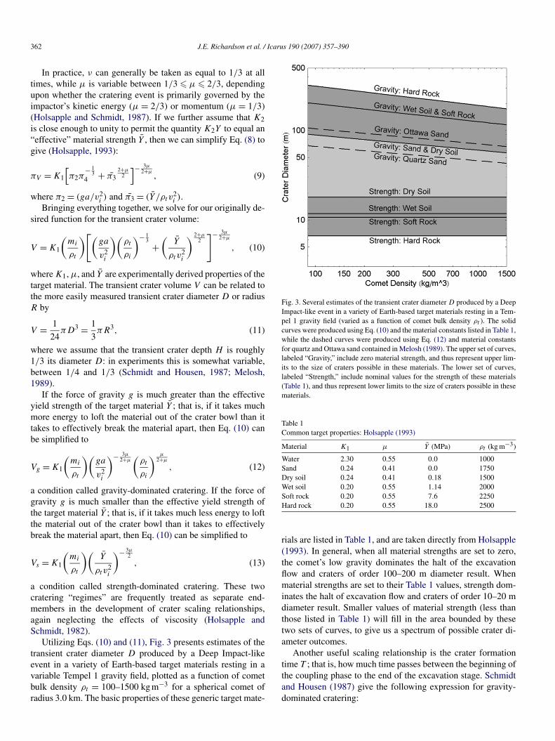
Utilizing Eqs. (10) and (11), Fig. 3 presents estimates of thetransient crater diameter D produced by a Deep Impact-likeevent in a variety of Earth-based target materials resting in avariable Tempel 1 gravity field, plotted as a function of cometbulk density ρt = 100–1500 kg m−3 for a spherical comet ofradius 3.0 km. The basic properties of these generic target mate-
Fig. 3. Several estimates of the transient crater diameter D produced by a DeepImpact-like event in a variety of Earth-based target materials resting in a Tem-pel 1 gravity field (varied as a function of comet bulk density ρt ). The solidcurves were produced using Eq. (10) and the material constants listed in Table 1,while the dashed curves were produced using Eq. (12) and material constantsfor quartz and Ottawa sand contained in Melosh (1989). The upper set of curves,labeled “Gravity,” include zero material strength, and thus represent upper lim-its to the size of craters possible in these materials. The lower set of curves,labeled “Strength,” include nominal values for the strength of these materials(Table 1), and thus represent lower limits to the size of craters possible in thesematerials.
Table 1Common target properties: Holsapple (1993)
Material K1 μ Y (MPa) ρt (kg m−3)
Water 2.30 0.55 0.0 1000Sand 0.24 0.41 0.0 1750Dry soil 0.24 0.41 0.18 1500Wet soil 0.20 0.55 1.14 2000Soft rock 0.20 0.55 7.6 2250Hard rock 0.20 0.55 18.0 2500
rials are listed in Table 1, and are taken directly from Holsapple(1993). In general, when all material strengths are set to zero,the comet’s low gravity dominates the halt of the excavationflow and craters of order 100–200 m diameter result. Whenmaterial strengths are set to their Table 1 values, strength dom-inates the halt of excavation flow and craters of order 10–20 mdiameter result. Smaller values of material strength (less thanthose listed in Table 1) will fill in the area bounded by thesetwo sets of curves, to give us a spectrum of possible crater di-ameter outcomes.
Another useful scaling relationship is the crater formationtime T ; that is, how much time passes between the beginning ofthe coupling phase to the end of the excavation stage. Schmidtand Housen (1987) give the following expression for gravity-dominated cratering:
Deep Impact ejecta plume analysis 363
(14)Tg = KTgl
(a
vi
)(ρt
ρi
)− 13(2+μ)
(ga
v2i
)− 1+μ2+μ
,
along with a more convenient “short-form” solution:
(15)Tg = KTg
√V 1/3
g.
A proportionality constant value of KT gl = 1.6 is given byMelosh (1989), derived from the data presented in Schmidt andHousen (1987), while in Fig. 9 of Schmidt and Housen (1987),an experimentally determined value of KTg = 0.8 is provided.Due to the “self-similarity” of all gravity-scaled craters, theseconstants are applicable to the full spectrum of impact environ-ments and target materials (from sand to hard rock), and weshall make use of constant KTg in Section 2.
With regard to strength-dominated cratering, Schmidt andHousen (1987) give the following long-form equation for thecrater formation time:
(16)Ts = KT sl
(a
vi
)(ρt
ρi
)− 13(
Y
ρtv2i
)− 1+μ2
.
while in Housen et al. (1983) we find the equivalent “short-form” version:
(17)Ts = KT sV13
√ρt
Y.
However, no values for the strength-dominated proportionalityconstants KT sl or KT s have been published in the literature,and even if they were, due to the non-similarity of strength-dominated craters, such constants would be limited to verysimilar experiments only.
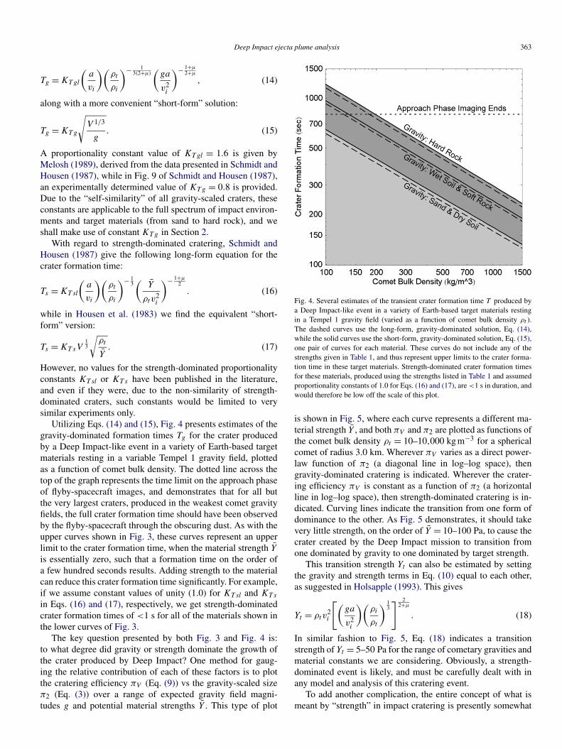
Utilizing Eqs. (14) and (15), Fig. 4 presents estimates of thegravity-dominated formation times Tg for the crater producedby a Deep Impact-like event in a variety of Earth-based targetmaterials resting in a variable Tempel 1 gravity field, plottedas a function of comet bulk density. The dotted line across thetop of the graph represents the time limit on the approach phaseof flyby-spacecraft images, and demonstrates that for all butthe very largest craters, produced in the weakest comet gravityfields, the full crater formation time should have been observedby the flyby-spacecraft through the obscuring dust. As with theupper curves shown in Fig. 3, these curves represent an upperlimit to the crater formation time, when the material strength Y
is essentially zero, such that a formation time on the order ofa few hundred seconds results. Adding strength to the materialcan reduce this crater formation time significantly. For example,if we assume constant values of unity (1.0) for KT sl and KT s
in Eqs. (16) and (17), respectively, we get strength-dominatedcrater formation times of <1 s for all of the materials shown inthe lower curves of Fig. 3.
The key question presented by both Fig. 3 and Fig. 4 is:to what degree did gravity or strength dominate the growth ofthe crater produced by Deep Impact? One method for gaug-ing the relative contribution of each of these factors is to plotthe cratering efficiency πV (Eq. (9)) vs the gravity-scaled sizeπ2 (Eq. (3)) over a range of expected gravity field magni-tudes g and potential material strengths Y . This type of plot
Fig. 4. Several estimates of the transient crater formation time T produced bya Deep Impact-like event in a variety of Earth-based target materials restingin a Tempel 1 gravity field (varied as a function of comet bulk density ρt ).The dashed curves use the long-form, gravity-dominated solution, Eq. (14),while the solid curves use the short-form, gravity-dominated solution, Eq. (15),one pair of curves for each material. These curves do not include any of thestrengths given in Table 1, and thus represent upper limits to the crater forma-tion time in these target materials. Strength-dominated crater formation timesfor these materials, produced using the strengths listed in Table 1 and assumedproportionality constants of 1.0 for Eqs. (16) and (17), are <1 s in duration, andwould therefore be low off the scale of this plot.
is shown in Fig. 5, where each curve represents a different ma-terial strength Y , and both πV and π2 are plotted as functions ofthe comet bulk density ρt = 10–10,000 kg m−3 for a sphericalcomet of radius 3.0 km. Wherever πV varies as a direct power-law function of π2 (a diagonal line in log–log space), thengravity-dominated cratering is indicated. Wherever the crater-ing efficiency πV is constant as a function of π2 (a horizontalline in log–log space), then strength-dominated cratering is in-dicated. Curving lines indicate the transition from one form ofdominance to the other. As Fig. 5 demonstrates, it should takevery little strength, on the order of Y = 10–100 Pa, to cause thecrater created by the Deep Impact mission to transition fromone dominated by gravity to one dominated by target strength.
This transition strength Yt can also be estimated by settingthe gravity and strength terms in Eq. (10) equal to each other,as suggested in Holsapple (1993). This gives
(18)Yt = ρtv2i
[(ga
v2i
)(ρi
ρt
) 13] 2
2+μ
.
In similar fashion to Fig. 5, Eq. (18) indicates a transitionstrength of Yt = 5–50 Pa for the range of cometary gravities andmaterial constants we are considering. Obviously, a strength-dominated event is likely, and must be carefully dealt with inany model and analysis of this cratering event.
To add another complication, the entire concept of what ismeant by “strength” in impact cratering is presently somewhat

364 J.E. Richardson et al. / Icarus 190 (2007) 357–390
Fig. 5. A plot of cratering efficiency πV (Eq. (2)) verses gravity-scaled sizeπ2 (Eq. (3)) for a Deep Impact-like event, where both πV and π2 are plot-ted as functions of comet Tempel 1’s bulk density ρt , ranging from 10 to10,000 kg m−3. Dry soil is used for the basic material parameters, and eachcurve represents a different value of the effective material strength Y . Theupper, bold curve shows the result of Y = 0 Pa and gravity-dominated cra-tering. Increasing this strength incrementally (the remaining curves) revealsa transition zone from gravity to strength domination between about 10 and100 Pa (curved lines), with strength dominating the cratering event completelyat strengths above these values (such as the Y = 1000 Pa line).
fuzzy. Modern theories of dynamic fracture indicate that the ac-tual failure strength of a material should be strongly rate depen-dent (Grady and Kipp, 1987), a factor not included in the deriva-tion of the crater scaling relationships. Additionally, CHD mod-eling indicates that the strength of the material surrounding animpact is often strongly degraded by shock-wave passage longbefore the excavation flow clears this material out of the craterinterior, such that the excavation stage is governed more by atarget’s “post-shock” strength than its initial strength (Croft,1981; Asphaug and Melosh, 1993; Nolan et al., 1996). Fur-thermore, impact energy expended in the compaction of poroustarget material will also manifest itself as a form of “strength,”since our current scaling relationships include only a genericstress variable Y , equivalent to an energy expended per unitvolume during crater formation, which does not specify howthat energy was actually used (Housen and Holsapple, 2003;Holsapple and Housen, 2007). We must therefore be careful torefer to any determined strength for the surface of Tempel 1 asan “effective” strength Y , and note that the value obtained willbe more of a nebulous yield strength (or energy density) than aspecific laboratory-referenced material strength—tensile, com-pressive, shear, or otherwise. With this qualification in mind, inthe next section we continue to make use of derived crateringevent scaling relationships to develop a model of cratering ex-cavation flow, which will include the effects of target materialstrength.
2. Model theoretical development
The primary focus of this study is, in effect, to solve a ballis-tics problem: where in this case we are not able to actually seethe individual projectiles (ejecta particles) in flight, but can in-stead only monitor the collective behavior of the ejecta particlesas they form a hollow, expanding, cone-shaped cloud. Nonethe-less, as with all ballistics problems, the primary variables fallinto two major categories: (1) the particle launch conditions,given by starting position, time, velocity, and launch angle; and(2) the forces on the particle in flight, dominated by the grav-ity field of the comet, but also including smaller forces, suchas solar radiation pressure. It is therefore convenient to breakthe description of the model into two sections, one describingthe theoretical development of the model (this section), whichgoes into establishing the launch conditions of the impact ejectaparticles; and one describing the computational development ofthe model (Section 3), which determines the forces on individ-ual particles once launched, and traces their flight over time toeither landing or escape.
2.1. The Maxwell Z-model of excavation flow
As mentioned in Section 1.1, the excavation flow-field es-tablished by the passage of the initial shock-wave and its sur-face reflection (rarefaction-wave), has very fluid-like (hydro-dynamic) properties. These properties were first modeled andexplored in detail for explosion craters by Maxwell and Seifert(1974) and then extended to impact craters by Maxwell (1977),in what became known as the Maxwell Z-model of crater ex-cavation. While our work is not a direct application of theMaxwell Z-model, there are many features of excavation flowfirst recognized in that model which we will take advantage ofin this work.
As stated in Maxwell (1977), there are two key, experimen-tally observed features of the cratering excavation flow:
• The transit of the ground shock through the incipient crater-ing region initiates a cratering flow-field that persists longafter the impulsive stresses have decayed.
• The associated cratering process can be approximated asincompressible flow along stationary streamlines.
Fig. 6 shows a graphical representation of the early stagesof crater excavation flow using the Maxwell Z-model, and de-picts 18 tracer particles strung like beads along seven differentflow streamlines (the arrowed lines) to illustrate the key fea-tures. These are:
• All particles at a given radial distance r from the impactsite will begin motion at the same speed. This is representedby the three contour lines (isotachs) connecting particles 1and 4, then 2 and 5, and finally 3 and 6, respectively, intime-step (a).
• For a normal-incidence (vertical) impact into a horizon-tally flat target, all streamlines will be axially symmetricabout the impact-point’s surface normal vector, producing

Deep Impact ejecta plume analysis 365
Fig. 6. Graphical representation of the Maxwell Z-model of excavation flow, adapted from a similar figure in Maxwell (1977). Depicted is the motion of 18 tracerparticles (six are numbered) over a short time period from the time of impact, as they move along seven hydrodynamic streamlines (the arrowed lines). All tracerparticles begin motion immediately after impact and flow-field establishment, and fall on three velocity contours: the three lines of constant radius shown in part (a).These streamlines are axially symmetric, producing “streamtubes” in three dimensions, such that the tracer particles will decelerate as they progress along theirrespective streamlines, which maintains the continuity of mass in a 3-D streamtube of increasing area. All particles in a given streamline, emerging from the groundsurface at some distance r from the impact site, will have the same ejection velocity (that of particles 1, 2, and 3).
“streamtubes” in three dimensions. As such, to maintain in-compressible flow and satisfy the continuity equation (con-servation of mass), flow velocity along each streamtubemust necessarily decrease with increasing distance from theimpact site, as the streamtube surface area increases.
• All particles in a given streamline will emerge from thesurface at the same, final, ejection velocity. That is, all par-ticles passing through the original ground surface at someradial distance r from the impact site will have the sameemergence velocity ve (speed and ejection angle). Thus, al-though particles 2 and 4 begin motion at different speeds,they will both be ejected at the same speed (that of par-ticle 2). The same thing holds true for particles 3 and 5,which also emerge at the same speed (that of particle 3).
• Although the flow in each streamline is steady-state and in-compressible, it is not inviscid: frictional forces betweenthe particles, and in particular, between particles in adja-cent streamlines, contribute to slowing the particles as theymove radially outward and curve upward.
• Once the particles in each streamline have moved abovethe original, ground surface level, they are considered tobe ballistically launched and all frictional forces betweenparticles are assumed to become negligible.
Each streamline in Fig. 6 has both a “leading edge,” indi-cated by particles 1, 2, and 3, and a “trailing edge” indicated bythe wall of the expanding crater cavity. As each streamline ap-proaches and then breaks the surface completely, shown by thestreamline containing particle 1 in time-step (b) and then by thestreamline containing particles 2 and 4 in time-step (c), the trail-
ing edge of that streamline will evolve from forming part of thecavity wall, to marking the cavity rim (upon emergence), and fi-nally to forming part of the ballistically launched ejecta plume.Also note that particles on the leading edge of each streamlinebecome ballistic ejecta immediately upon flow-field establish-ment.
With time and the development of computational hydrody-namic (CHD) codes, the Maxwell Z-model lost much of itsutility because at its best, it represents only a good first-orderdescription of cratering excavation flow and lacks many of thefiner variations present in even a simple cratering event (Croft,1980; Austin et al., 1980). Nonetheless, many of the experi-mentally observed features contained in the Maxwell Z-modelcontinue to be valid, and we shall refer to this section frequentlyin the development of our own, scaling-relation based model. Incontrast to the Z-model, our model will deal only with particlebehavior at the point of launch (that is, as the particles leavethe level of the original ground surface), and thereafter. Exca-vation flow-field behavior prior to this point (below the groundsurface) is left to the CHD modelers, who have a much morecapable tool for handling those details.
2.2. Impact ejecta scaling relationships
Our first task is to determine the correct particle ejection(launch) velocities for a given impact event. To accomplish thiswe utilize eight of the equations given in Table 1 of Housen etal. (1983), which were developed using the dimensional analy-sis techniques described in Section 1.3 to scale and model thebehavior of impact ejecta. These scaling relationships, how-
366 J.E. Richardson et al. / Icarus 190 (2007) 357–390
ever, lack numerical values for their proportionality constants,and we must therefore find a way to fix each constant’s valuein terms of some experimentally determined constants. Forthis exercise, we will continue to use the material constant μ
from Section 1.3, and include the constant KTg from Eq. (15)(Schmidt and Housen, 1987).
To describe the launch position, time, and velocity of bothleading and trailing edge ejecta in the gravity-dominated crater-ing regime, we will use four of the relationships from Table 1 ofHousen et al. (1983), beginning with the equation for the craterformation time Tg :
(19)Tg = CTg
√Rg
g,
where Rg is the gravity-dominated transient crater radius deter-mined from Eqs. (10) and (11). We can immediately recognizethe similarity of Eq. (19) to Eq. (15) and determine that
(20)CTg = KTg
(π
3
) 16
,
for a crater in which the transient crater has a depth to diameterratio of 1/3. In effect, CTg ≈ KTg within experimental accu-racy.
Now we take advantage of the relationship of Eq. (19) to thegiven equation for plume position r as a function of time t inHousen et al. (1983):
(21)r(t) = CpgRg
(t
√g
Rg
) μμ+1
,
where t is the time after impact, and we have replaced the givenexponent α with its equivalent form of α = 3μ/(2 + μ) fromHolsapple and Schmidt (1987). There are two important thingsto note about Eq. (21). First, we define the “plume position”referred to in Table 1 of Housen et al. (1983) as the base ofthe trailing edge of the ejecta plume, which progresses in nearpower-law fashion from the impact site toward the transientcrater rim. Second, as discussed in Section 2.1, the base of thetrailing edge of the ejecta plume also marks the cavity rim po-sition, such that the bowl of the growing crater and the trailingedge of the ejecta plume form a continuous, moving surfaceduring crater growth (Fig. 6).
We can solve for the constant Cpg by assuming that the craterexhibits power-law growth all the way out to the transient craterrim at Rg . This is not entirely the case, due to the forces ofstrength and/or gravity slowing the growth near the transientcrater rim (Holsapple and Schmidt, 1987; Schmidt and Housen,1987), but this approximation works reasonably well, especiallysince the cavity rim approaches this point asymptotically. Ac-cepting this assumption, we set t = Tg and r = Rg in Eq. (21)to obtain the following expression for the constant Cpg:
(22)Cpg = C− μ
μ+1Tg .
The cavity rim position expression, Eq. (21), is also usefulin that the speed at which the crater rim advances must neces-sarily be equal to the horizontal velocity component veh of the
ejecta which is, at that moment, just leaving the rim to join theejecta plume (Section 2.1). Thus, by taking the first derivativeof Eq. (21) we obtain:
(23)veh(t) = Cpg
(μ
μ + 1
)√gRg
(t
√g
Rg
)− 1μ+1
.
The total ejection velocity can be obtained if we know theparticle ejection angle ψ (measured from the horizontal) byusing ve = veh secψ . For this constant derivation exercise, weadopt a mean ejection angle of ψ ≈ 45◦, an assumption whichdates back to the original Z-model (Maxwell and Seifert, 1974).Actual ejection angles vary with distance r (Section 2.4), butthis assumption holds reasonably well for the materials that weare considering here. This gives
(24)ve(t) = C− μ
μ+1Tg
√2
(μ
μ + 1
)√gRg
(t
√g
Rg
)− 1μ+1
,
which has the same form as that given in Housen et al. (1983)for the ejection velocity as a function of time:
(25)ve(t) = Cvtg√
gRg
(t
√g
Rg
)− 1μ+1
,
and by comparison we find that
(26)Cvtg = C− μ
μ+1Tg
√2
(μ
μ + 1
).
At this point we have obtained an expression for the parti-cle ejection velocity as a function of time t for the trailing edgeof the ejecta plume (at the advancing cavity rim). However, theejecta on the leading edge of the ejecta plume are launched im-mediately (effectively at time t = 0), so we must next obtain anexpression for the particle ejection velocity ve as a function ofposition r . To do this, we first rearrange the cavity rim positionEq. (21) to solve for the time t :
(27)t (r) = CTg
√Rg
g
(r
Rg
)μ+1μ
.
Note that if we let r go to Rg in Eq. (27), we recover ourprevious expression for the gravity-dominated crater formationtime Tg (Eq. (19)). Equation (27) serves two important purposesin our model: first, it gives us the ejection time t as a functionof rim position r for particles on the trailing edge of the ejectaplume; second, it serves as a good approximation for the craterformation time Ts in strength-dominated cratering events, byletting r = Rs and solving for the time t .
If we substitute the ejection time expression, Eq. (27), intothe ejection velocity expression, Eq. (25), we obtain an expres-sion for the ejection velocity ve as a function of position r :
(28)ve(r) =√
2
CTg
(μ
μ + 1
)√gRg
(r
Rg
)− 1μ
.
Equation (28) has the same form at that given in Housen et al.(1983) for the gravity-dominated ejection velocity as a function
Deep Impact ejecta plume analysis 367
of position:
(29)ve(r) = Cvpg√
gRg
(r
Rg
)− 1μ
,
and by comparison, we obtain an expression for the proportion-ality constant:
(30)Cvpg =√
2
CTg
(μ
μ + 1
).
Thus, we can now describe the launch position, time, andvelocity of both leading and trailing edge ejecta in the gravity-dominated cratering regime. We can perform this same exer-cise for the four equations describing impact ejecta behaviorin the strength-dominated cratering regime, given in Table 1 ofHousen et al. (1983), to obtain:
Crater formation time (strength regime):
(31)Ts = CT sRs
√ρt
Y,
where Rs is the strength-dominated transient crater radius, de-termined using Eqs. (10) and (11), and
(32)CT s = KT s
(π
3
) 13
.
Ejecta plume trailing edge, or cavity rim position (strengthregime):
(33)r(t) = CpsRs
(t
Rs
√Y
ρt
) μμ+1
,
where
(34)Cps = C− μ
μ+1T s .
Ejecta velocity as a function of time for the plume trailingedge (strength regime):
(35)ve(t) = Cvts
√Y
ρt
(t
Rs
√Y
ρt
)− 1μ+1
,
where
(36)Cvts = C− μ
μ+1T s
√2
(μ
μ + 1
).
Ejection velocity as a function of emergence position(strength regime):
(37)ve(r) = Cvps
√Y
ρt
(r
Rs
)− 1μ
,
where
(38)Cvps =√
2
CT s
(μ
μ + 1
).
There is, however, an important distinction between thesefour equations for the strength regime and the previous four
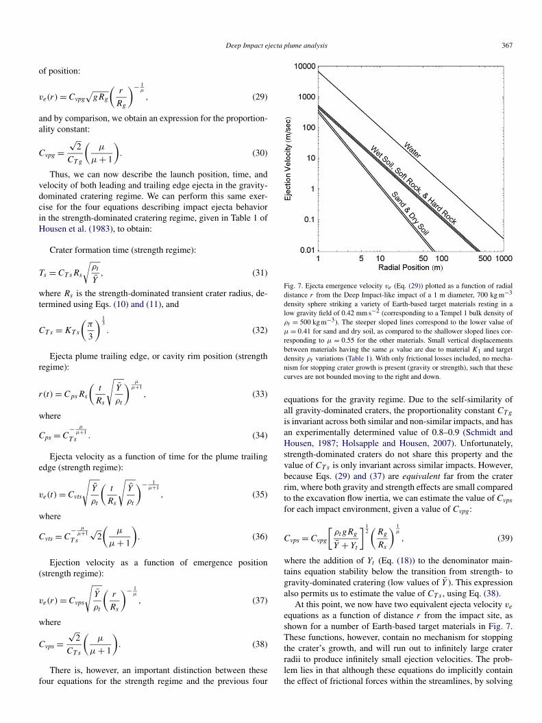
Fig. 7. Ejecta emergence velocity ve (Eq. (29)) plotted as a function of radialdistance r from the Deep Impact-like impact of a 1 m diameter, 700 kg m−3
density sphere striking a variety of Earth-based target materials resting in alow gravity field of 0.42 mm s−2 (corresponding to a Tempel 1 bulk density ofρt = 500 kg m−3). The steeper sloped lines correspond to the lower value ofμ = 0.41 for sand and dry soil, as compared to the shallower sloped lines cor-responding to μ = 0.55 for the other materials. Small vertical displacementsbetween materials having the same μ value are due to material K1 and targetdensity ρt variations (Table 1). With only frictional losses included, no mecha-nism for stopping crater growth is present (gravity or strength), such that thesecurves are not bounded moving to the right and down.
equations for the gravity regime. Due to the self-similarity ofall gravity-dominated craters, the proportionality constant CTg
is invariant across both similar and non-similar impacts, and hasan experimentally determined value of 0.8–0.9 (Schmidt andHousen, 1987; Holsapple and Housen, 2007). Unfortunately,strength-dominated craters do not share this property and thevalue of CT s is only invariant across similar impacts. However,because Eqs. (29) and (37) are equivalent far from the craterrim, where both gravity and strength effects are small comparedto the excavation flow inertia, we can estimate the value of Cvps
for each impact environment, given a value of Cvpg:
(39)Cvps = Cvpg
[ρtgRg
Y + Yt
] 12(
Rg
Rs
) 1μ
,
where the addition of Yt (Eq. (18)) to the denominator main-tains equation stability below the transition from strength- togravity-dominated cratering (low values of Y ). This expressionalso permits us to estimate the value of CT s , using Eq. (38).
At this point, we now have two equivalent ejecta velocity ve
equations as a function of distance r from the impact site, asshown for a number of Earth-based target materials in Fig. 7.These functions, however, contain no mechanism for stoppingthe crater’s growth, and will run out to infinitely large craterradii to produce infinitely small ejection velocities. The prob-lem lies in that although these equations do implicitly containthe effect of frictional forces within the streamlines, by solving
368 J.E. Richardson et al. / Icarus 190 (2007) 357–390
for the streamline emergence velocity ve, they do not containthe effects of gravity and material strength, which are whatultimately halts the growth of the crater. This issue will be ad-dressed in the next section.
2.3. The end of crater excavation
To bring in the effects of gravity g and strength Y and haltthe crater’s growth, we take advantage of a basic concept de-scribed in the Maxwell Z-model (Section 2.1); namely, that theejecta flow emerging from the surface at some radius r fromthe impact site represents a hydrodynamic streamline, which issteady state and incompressible. If we also assume that fric-tional forces beyond those implicit in Eqs. (29) and (37) aresmall compared to the forces of inertia, gravity, and strength(that is, inviscid flow), we can use Bernoulli’s principle at thepoint of ejecta emergence to form an energy balance equation:
(40)1
2ρtv
2ef = 1
2ρtv
2e − Kgρtgr − KsY ,
where ve is the emergence velocity (after losses due to fric-tion), and vef is the effective ejection velocity that we desire(after losses due to gravity and strength). Beginning on the left,the first two terms describe the kinetic energy (or stagnationpressure) of the excavation flow in a single streamline, assum-ing that upon emergence, the hydrostatic pressure in the flow iszero. The third term describes the mean amount of gravitationpotential energy needed to loft each unit volume in the flow (afunction of surface radius r), and the fourth term describes theamount of energy needed to fracture or “break loose” each unitvolume in the flow (a function of effective target strength Y ).We do, however, have two new constants to solve for: Kg
and Ks .By substituting Eq.( 29) for ve in Eq. (40), we can solve for
the value of Kg by setting the target strength Y to zero (assumegravity-dominated cratering) and then let the crater radius r goto Rg as the effective velocity vef goes to zero (halting cratergrowth). This gives us Kg = C2
vpg/2. In similar fashion, we cansubstitute Eq. (37) for ve in Eq. (40), and solve for the valueof Ks by setting the target gravity g to zero (assume strength-dominated cratering) and then let the crater radius r go to Rs asthe effective velocity vef goes to zero. This gives Ks = C2
vps/2.Plugging these values into Eq. (40) yields:
(41)vef (r) =[v2e − C2
vpggr − C2vps
Y
ρt
] 12
.
In examining Eqs. (40) and (41), we can ask: do our valuesfor Kg and Ks make physical sense? The value of Kgr rep-resents a mean streamline excavation depth, and ranges fromr/9.0 (at μ = 0.40) to r/5.8 (at μ = 0.55) for a CTg value of0.85. This implies maximum streamline excavation depths ofr/4.5 to r/2.9, which is certainly reasonable: usual values rangefrom r/5 to r/4 (Melosh, 1989). The value of KsY representsa post-shock “yield” strength for the target material and, due tothe variant nature of CT s , can range from Y /3 to Y /15, withvalues from Y /5 to Y /10 being typical. These values are lessthan the Tresca maximum shear stress criteria of Y/2 (Turcotte
and Schubert, 2002), assuming that the primary stress duringexcavation flow is shear stress between adjacent streamlines,but could be reasonable for such “pre-damaged” target material.Both of these constants (Kg and Ks ) are deliberately consistentwith the previous crater-size scaling relationships (Section 1.3),such that as the computed transient crater rim distance R is ap-proached, determined by Eqs. (10) and (11), ejecta velocitiesare properly slowed to zero.
Another way to check our velocity braking function isto look for “overturn-flap” behavior near the rim of gravity-dominated events (Croft, 1980; Melosh, 1989). That is, near therim of simple, gravity-dominated craters, the last material to beejected and then redeposited moves in such a way as to maintainits radial and vertical integrity, and thus produces a hinge-likeoverturn-flap of material visible at the final crater rim. This canbe described functionally by a simple ballistics equation:
(42)vo =[
2g(Rg − r)
sin(2ψ)
] 12
,
where vo is the velocity necessary to land a particle at the samedistance beyond the transient crater rim as it began inside of thetransient crater rim, in an environment with a flat surface anduniform gravity field. Our effective ejection velocity vef func-tion (Eq. (41)) shows good agreement with this overturn-flapfunction vo (Eq. (42)) over the final 10–20% of crater growth ingravity-dominated events, consistent with the geological obser-vations. Conversely, by insisting upon good agreement with theoverturn-flap function (Eq. (42)) over the final stages of tran-sient crater growth, we can constrain the value of constant KTg
to a range of 0.75–0.95, in good agreement with this constan-t’s experimentally determined values of 0.8–0.9 (Schmidt andHousen, 1987; Holsapple and Housen, 2007).
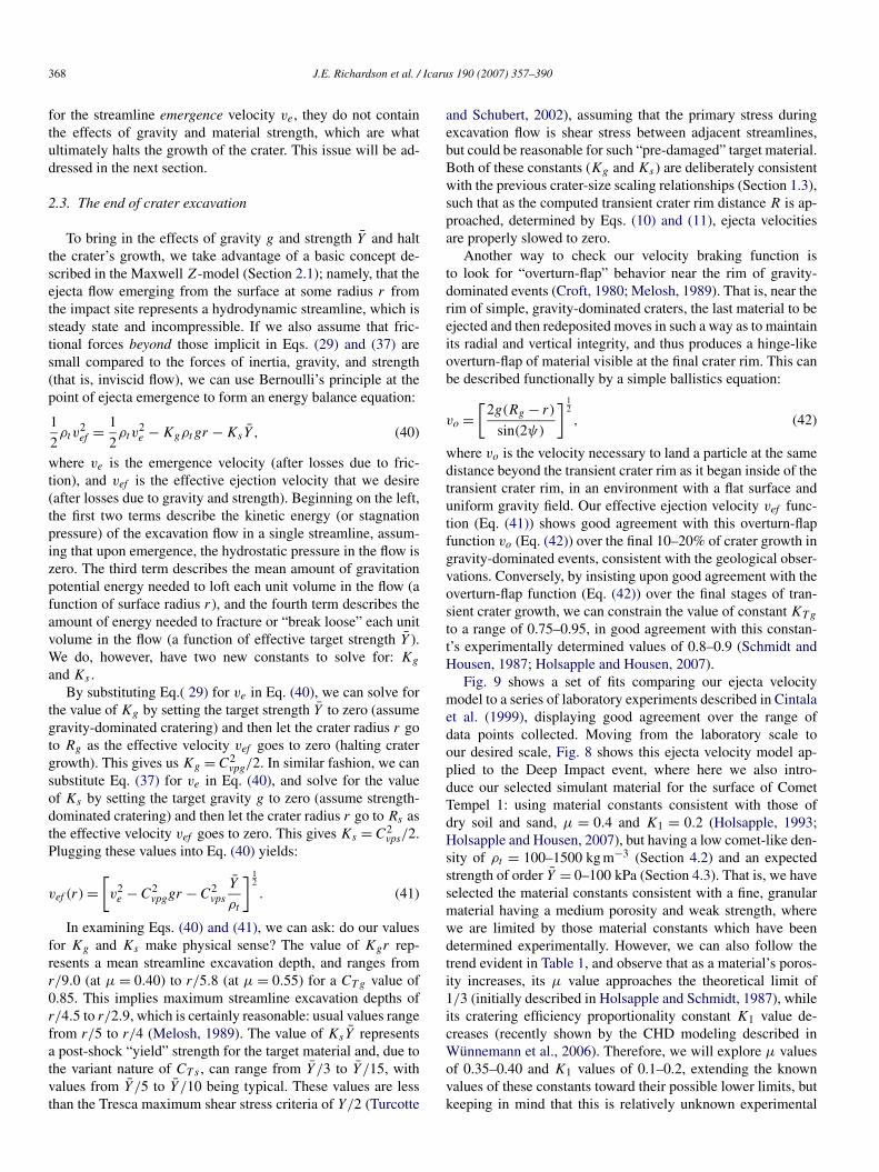
Fig. 9 shows a set of fits comparing our ejecta velocitymodel to a series of laboratory experiments described in Cintalaet al. (1999), displaying good agreement over the range ofdata points collected. Moving from the laboratory scale toour desired scale, Fig. 8 shows this ejecta velocity model ap-plied to the Deep Impact event, where here we also intro-duce our selected simulant material for the surface of CometTempel 1: using material constants consistent with those ofdry soil and sand, μ = 0.4 and K1 = 0.2 (Holsapple, 1993;Holsapple and Housen, 2007), but having a low comet-like den-sity of ρt = 100–1500 kg m−3 (Section 4.2) and an expectedstrength of order Y = 0–100 kPa (Section 4.3). That is, we haveselected the material constants consistent with a fine, granularmaterial having a medium porosity and weak strength, wherewe are limited by those material constants which have beendetermined experimentally. However, we can also follow thetrend evident in Table 1, and observe that as a material’s poros-ity increases, its μ value approaches the theoretical limit of1/3 (initially described in Holsapple and Schmidt, 1987), whileits cratering efficiency proportionality constant K1 value de-creases (recently shown by the CHD modeling described inWünnemann et al., 2006). Therefore, we will explore μ valuesof 0.35–0.40 and K1 values of 0.1–0.2, extending the knownvalues of these constants toward their possible lower limits, butkeeping in mind that this is relatively unknown experimental
Deep Impact ejecta plume analysis 369
Fig. 8. Modeled ejecta velocities as a function of radial distance r from the Deep Impact-like impact of a 1 m diameter, 700 kg m−3 density sphere striking acomet-simulant target (ρt = 500 kg m−3) resting in a low gravity field of 0.42 mm s−2: shown in both linear (left) and log (right) format. Legend: thin solidline = emergence velocity curve ve (Eq. (29)); thin dotted line = overturn-flap function vo (Eq. (42)), hinged at the computed gravity-dominated crater radius Rg ;thick solid line = zero-strength (gravity-dominated) effective velocity curve vef (Eq. (41)); thick dot–dash lines = effective velocity curve vef (Eq. (41)) at strengthsof (0 dot) 0.5 kPa, (1 dot) 5 kPa, (2 dots) 50 kPa, and (3 dots) 500 kPa; thin dashed lines = computed strength-dominated crater radii Rs for these same strengthvalues.
territory. Table 2 lists the input parameters that we have devel-oped for the model so far.
2.4. Impact ejecta launch angles
To determine a useful expression for the particle ejectionangle ψ (measured from the horizontal target surface) as afunction of distance r we will need to rely heavily upon pastexperimental results and fits to their data. There are currentlyno scaling relations known for this aspect of impact cratering,and in fact, Housen et al. (1983) simply assume an unspecified,constant ejection angle. Much of the literature on this topic is inregard to excavation flow studies using the Maxwell Z-model,where the particle ejection angle is related to the parameter Z
by (Maxwell and Seifert, 1974; Maxwell, 1977):
(43)ψ = tan−1(Z − 2),
such that for Z = 3, ψ = 45◦. Most instances in the litera-ture place Z at between 2.5 and 4 near the surface, for ejectionangles of between 27◦ and 63◦. Here is a summary of the high-lights:
• Thomsen et al. (1980b) found that for an impact whichpenetrates below the surface, ejection angles should de-crease as a function of r in hyperbolic fashion; rapidly atfirst, and then leveling off. They obtained Z values of 3–4(ψ = 45◦–63◦) near the surface for their experiment.
• Thomsen et al. (1980a) determined a best-fit surface Z =2.7 (ψ = 35◦) from one experiment.
• Croft (1980) determined a best-fit surface Z = 2.5–2.9(ψ = 35◦–39◦) from crater and ejecta-blanket models ofthe Meteor Crater and Prairie Flat events.
• Austin et al. (1981) found, in Lagrangian calculations ofexcavation flow, that Z-values near the surface fall into therange of Z = 2.5–3.0 (ψ = 35◦–45◦) by simulating smalllaboratory experiments.
• Cintala et al. (1999) used strobed laser-light images to di-rectly measure the flight of large, coarse sand particles innormal-incidence laboratory impacts, to find that ejectionangles generally decrease over crater growth: beginning atabout 45◦–55◦ at 0.2 Rg and dropping to about 35◦–45◦ at0.6 Rg (Figs. 9 and 11).
• Anderson et al. (2003) used a laser imaging system to di-rectly measure the flight of fine sand particles in normal-and oblique-incidence laboratory impacts, to find thatnormal-incidence ejection angles generally decrease overcrater growth: beginning at about 52◦ at 0.2 Rg and drop-ping to about 44◦ at 0.5 Rg .
There seems to be widespread agreement in the literaturethat particle ejection angles decrease over the course of cratergrowth, but the form of that decrease is not so clear. Early mod-elers, such as Thomsen et al. (1980b) assumed that Z near thesurface is constant, but that the initial depth-of-burial of the im-pactor would create initially high ejection angles, which thenrapidly decrease with increasing r to stabilize at some constantvalue. More recent laboratory experiments, such as those de-scribed in Cintala et al. (1999) and Anderson et al. (2003), showa roughly linear decrease in ejection angles over the first half of

370 J.E. Richardson et al. / Icarus 190 (2007) 357–390
Fig. 9. Top row: a comparison of our ejecta velocity model (Eq. (41)) with three of the seven shots described in Cintala et al. (1999), showing good agreementwith each. Legend: thin solid line = emergence velocity curve ve (Eq. (29)); thin dotted line = overturn-flap function vo (Eq. (42)), hinged at the computedgravity-dominated crater radius Rg ; thick solid line = zero-strength (gravity-dominated) effective velocity curve vef (Eq. (41)); thin dashed line = computedgravity-dominated crater radius Rg . Bottom row: linear, least-squares fits to the ejection angle data from three of the seven shots described in Cintala et al. (1999),demonstrating that a linearly decreasing ejection angle as a function of radius r is a reasonable assumption for each shot.
Table 2Model input parameters
Name Symbol Nominal value Value range
Impactor radius a 0.5 m –Impactor density ρi 700 kg m−3 –Impactor mass mi 366 kg –Impactor speed vi 10.2 km s−1 –Impact angle φ 34◦ 29◦–39◦Scaling constant μ 0.4 0.35–0.4Scaling constant K1 0.2 0.1–0.2Scaling constant KTg 0.85 0.75–0.95
cavity growth, but these appear to level off or even turn upwardagain as cavity growth continues. However, because these lab-oratory experiments take place in small target containers, theseexperiments may be seeing the effects of shock-wave reflectionfrom the bottom and sides of those containers. The shock-wavereflection from the bottom of the container would tend to addto the vertical component of ejecta velocities, while the shock-wave reflection from the side of the container would tend tosubtract from the radial component of ejecta velocities: botheffects tending to increase particle ejection angles. The low-
est speed ejecta, near the end of crater growth, would be themost susceptible to this effect, such that the leveling-off, and inparticular, the upturn in ejection angles near the end of cratergrowth may be an artifact of the laboratory environment.
Very recent CHD modeling, described in Collins and Wün-nemann (2007), indicates a continuous, monotonically decreas-ing ejection angle with cavity growth. Their numerical simu-lations display a drop of about 5◦–10◦ between 0.2 and 08 Rg ,without any leveling-off or upturn, and where the initial ejectionangle is dependent upon the material’s internal friction coef-ficient. For our first-order ejecta plume model, therefore, weadopt a simple, linearly decreasing ejection angle ψn for im-pacts at normal incidence, as a function of distance r from theimpact site:
(44)ψn(r) = ψo − ψd
(r
Rg
),
where the values for the starting angle ψo and total drop ψd willbe adjusted during the course of our forward model iterations(Section 4.1.2). As a starting point, we will use the seven labo-ratory shots described in Cintala et al. (1999), which in their lin-ear, least-squares fits show starting angles of ψo = 52.4◦ ± 6.1◦

Deep Impact ejecta plume analysis 371
and total angular drops of ψd = 18.4◦ ± 8.2◦, using 2σ errors(Fig. 9).
2.5. The effects of oblique impact
The last ingredient needed prior to handing the model off tothe three-dimensional motion integrator (Section 3) is to add inthe first-order effects of an oblique impact. This is importantto this study because the impactor–spacecraft for Deep Impactstruck the regional surface at an impact angle of φ = 34◦ ± 5◦(measured from the horizontal). Such an oblique impact willaffect the cratering event in four basic ways: the transient cratervolume and size will be smaller; particle ejections angles willbe lowered on the down-range side of the ejecta plume; particleejection velocities will be higher on the down-range side of theejecta plume; and the ejecta plume mass-loading will be shiftedtoward the down-range side. The first three of these effects canbe reasonably approximated and included in our model.
For some time now, it has been recognized that craters pro-duced by oblique impacts will maintain their circular shape andparaboloid profiles all the way down to impact angles of φ ≈10◦–15◦ (Gault and Wedekind, 1978; Pierazzo and Melosh,2000). This is because, as described in Sections 1.1 and 2.1, theestablished excavation flow-field is a function of two things:the outwardly propagating shock-wave generated by the im-pact, which will maintain a hemispherical shape and appear tooriginate from a point-source even in oblique impacts; and therarefaction-wave, which is a function of shock-wave reflectionfrom the free surface of the target (regardless of impact angle).The obliqueness of the impact does, however, play an impor-tant role in determining the amount of impactor energy andmomentum which goes into setting up the overall crater excava-tion. In an extensive series of experiments, Gault and Wedekind(1978) showed that it is the vertical component of the im-pactor’s kinetic energy and momentum which governs the cratersize, following a simple sine relationship: a result also sup-ported by more recent work (Chapman and McKinnon, 1986;Elbeshausen et al., 2007). As such, our applications of the crater(Section 1.3) and ejecta (Section 2.2) scaling relations will usevi sinφ to obtain the applicable component of the impactor’svelocity.
On the other hand, some fraction of the horizontal compo-nent of the impactor’s kinetic energy and momentum is trans-ferred to the excavation flow-field, such that it causes an in-crease in down-range directed, horizontal particulate motionand manifests itself as an overall increase in velocities and alowering of particle ejection angles on the down-range side ofthe ejecta plume. With regard to how much ejection angles andvelocities change with impact obliqueness, there are no scal-ing relationships to draw upon: only direct experimentation andsome three-dimensional CHD models. For this work, we willmake use of the recently published experimental data on ejec-tion angles and velocities contained in Anderson et al. (2003),Anderson et al. (2004), and Schultz et al. (2005) to producean empirical rule for use in our model. This function uses analtitude-azimuth coordinate system, where r is the particle dis-tance from the impact site, θ is the particle azimuth as mea-
sured from the direction of the incoming projectile, and φ isthe impact angle of the projectile (normal incidence occurs atφ = 90◦):
(45)ψf (r, θ) = ψn −[
30◦(cosφ)
(1 − cos θ
2
)(1 − r
Rg
)2].
The change in the overall ejection velocity for a particleis determined directly from this change to its ejection angle(Eq. (45)), assuming that all of this ejection angle change is theresult of an addition made to the horizontal velocity componentof the particle. The final ejection velocity vf at oblique-impactincidence, as a function of the final ejection angle ψf , is thusgiven by:
(46)vf (r, θ) =[(vef sinψn)
2 +(
vef sinψn
tanψf
)2] 1
2
.
Fig. 10 shows a plot of Eqs. (45) and (46) for a projectilecoming in at φ = 30◦, as compared to the experimental datapublished in Anderson et al. (2003). While the fit is reason-able, it is certainly not excellent, particularly where velocitiesare concerned in the later stages of measured plume expansion.However, this is at least a first step toward incorporating theseeffects into an impact ejecta model, and the fit does verify thatthe majority of the change in ejection angles and velocities oc-curs through a down-range directed addition to the horizontalvelocity component of the ejecta.
One final effect which will not be included in this modelis the down-range shift in ejecta plume mass-loading that isseen both in experiments and in its effect on the ejecta blan-kets of existing simple craters (Melosh, 1989; Pierazzo andMelosh, 2000). Below about φ = 45◦, the ejecta plume (and re-sulting ejecta deposit) becomes increasingly asymmetrical andbegins to develop a gap in its up-range side, called a “forbid-den zone” or “zone-of-avoidance.” This gap becomes largerand more prominent at lower impact angles, and at very lowimpact angles (φ < 5◦), the ejecta plume also develops a down-range gap, which produces a “butterfly” pattern in the resultingejecta blanket (Pierazzo and Melosh, 2000). The Deep Impactevent, impacting at φ = 34◦ ± 5◦ above the regional horizon,almost certainly produced an asymmetrical ejecta distribution,and hints of an up-range gap can be seen in the ejecta plume im-ages. However, at this stage in the science, we lack the meansto include even a simple, empirically based modification to themodel to incorporate this effect, and this omission should bekept in mind when comparing the simulation to the actual im-ages.
3. Model computational development
Up to this point, we have described only the theoreticaldevelopment of the model, which goes into establishing thelaunch conditions of the impact ejecta particles. In this sec-tion, we describe the computational development of the model,which determines the forces on the individual particles oncelaunched, and traces their flight over time to either landing orescape.

372 J.E. Richardson et al. / Icarus 190 (2007) 357–390
Fig. 10. The effects of a φ = 30◦ oblique impact on particle ejection angles (left) and normalized ejection velocities (right), both shown as a functions of azimuthangle from the impactor direction θ , where each pair of curves shows the effect on ejecta produced at different distances r from the impact site. The data points aretaken from Anderson et al. (2003), shown with 1σ error bars, while the curves represent our empirical function fit to this data set, given by Eqs. (45) and (46). Forthis data set, the best fit to ψn (Eq. (44)) occurs at ψo = 60◦ and ψd = 30◦ .
3.1. Ejecta plume behavior in two dimensions
The simplest form of this ejecta behavior model is one whichoperates in two spatial dimensions (horizontal and vertical mo-tion only), under the influence of a uniform gravity field. Thispermits us to use the standard equations of motion for ballis-tic flight (flat target-surface and no atmospheric drag effects)to simulate the ejecta behavior produced by small, vacuum-chamber, laboratory experiments done on Earth. Under thesesimple conditions, the equations of motion become:
(47)x(t) = xl + vf cosψf (t − tl),
(48)y(t) = vf sinψf (t − tl) − 1
2g(t − tl)
2,
where x and y are the horizontal and vertical ejecta particlepositions, respectively; xl is the horizontal launch position ofthe ejecta particle; and tl is the launch time of the ejecta particle.
To start the model, ten inputs are required: four for the im-pactor (a, ρi , vi , φ), four for the target surface (ρt , Y , μ,K1), the gravity field magnitude g, and the crater-centered az-imuth of the ejecta plume “slice” to be studied θ . From theseinputs, the transient crater volumes Vg and Vs are computed us-ing Eq. (10), for both the condition of zero strength and theuser supplied strength value Y . These two volumes are thenconverted to transient crater radii Rg and Rs (Eq. (11)), respec-tively, where both crater radii are needed by the ejecta scaling
relationships (Sections 2.2 and 2.3). Next, the desired crater ra-dius r is populated with two sets of several thousand tracer par-ticles, each assigned a launch position xl between the projectileradius a and transient crater radius Rs , with a launch veloc-ity vf (Eq. (46)) and ejection angle ψf (Eq. (45)) computed foreach particle. One set of tracer particles are used to mark the po-sition of the leading edge of the ejecta plume, and are launchedat time tl = 0. The second set of tracer particles are used tomark the position of the trailing edge of the ejecta plume, andare launched sequentially at time tl = t (r) from Eq. (27). Thisform of the model is easily handled by a computational mathe-matics package, such as Maple, Matlab, or Mathematica, withthe result displayed using standard plotting techniques.
Fig. 11 shows a comparison of this form of the model to asmall laboratory shot described in Cintala et al. (1999). The up-per two panels of this figure show a one-to-one matching of themodel to the photograph of shot 4035, with excellent agreement(only the leading edge of the ejecta plume is depicted in thesepanels). The lower two panels expand upon this laboratory-shot recreation and show both the leading and trailing edgesof the ejecta plume, along with the trajectories of some indi-vidual tracer particles, under conditions of both gravity- andstrength-dominated cratering. The model does a very good jobof displaying the evolution of the ejecta plume shape through-out crater growth, without having to model the streamline flowbelow ground level (compare the lower left panel of Fig. 11

Deep Impact ejecta plume analysis 373
Fig. 11. (Upper left) A photograph of shot 4035 from Cintala et al. (1999), into fine sand, where the leading edge of the impact ejecta plume is illuminated fromthe right by a vertical sheet of laser light, which was turned on for 0.2 ms at 2 ms intervals. The large arrow marks the approximate location of the transient craterrim, while small arrows mark the ballistic path of a few large particles. (Upper right) A model recreation of shot 4035 (Cintala et al., 1999), with the position ofthe ejecta plume’s leading edge shown at 2 ms intervals. The bold line marks the position of the plume at crater formation time Tg . All distances in these plots arenormalized to the crater radius Rg . (Lower left) A model of the same shot, only in these lower plots, larger scales are shown and both leading and trailing ejectaplume edges are modeled (and filled between). Dotted lines mark the ballistic path of the particles in nine individual streamlines. All times are normalized to thecrater formation time Tg . (Lower right) A model of the same shot again, but with Y = 10 kPa of strength added to the target. Although this creates a crater of abouthalf the diameter as before, and a much thinner ejecta plume, the plume advances at roughly the same rate.
to Fig. 6). Of key importance to the analysis of the Deep Im-pact event is the effect of adding strength to the model (thelower right panel): while the mass-loading in the ejecta plumeis significantly decreased, resulting in a thinner ejecta plume inthe simulation, the advancement rate of the plume is not sig-nificantly affected. This is because the particles which makeup the plume in its later advancement stages are ejected earlyenough in the process to have a high inertia (kinetic energy)and are not significantly effected by either strength or grav-ity in Eq. (41). To simulate the Deep Impact event, however,a more sophisticated form of the model is required, which op-erates in three spatial dimensions and can trace the motion ofeach tracer particle under the influence of the non-uniform grav-ity field produced by a small, rotating, irregular target body.
3.2. The ejecta plume as a polygon shape-model
To bring our ejecta plume model into three dimensions, weintroduce the concept of modeling the ejecta plume as a poly-
gon shape-model. Rather than using thousands of randomlyplaced tracer particles to mark the ejecta plume, such as in pre-vious studies (Geissler et al., 1996; Durda, 2004), we insteadlaunch two networks of tracer particles, one network to depictthe leading edge of the ejecta plume, and one to depict thetrailing edge of the ejecta plume. The tracer particles in eachnetwork are connected to form the vertices of triangular poly-gons which are, in turn, connected to form a continuous surfacefor both leading and trailing sides of the plume. To be more spe-cific, the polygon ejecta plume is made by placing two meshesof 1800 regularly spaced tracer particles on the starting surfacearea of the computed transient crater, such that 3540 triangu-lar polygons are formed in each mesh (these meshes initially lieone directly on top of the other). For each mesh, this arrange-ment creates 59 radial rings of 60 polygons each, ranging fromone projectile diameter d to the transient crater radius Rs in dis-tance from the impact site. The 2d diameter hole in the centerof the mesh is intentional, to avoid the region of potential va-por plume creation (Section 1.1). Particles in the top mesh are

374 J.E. Richardson et al. / Icarus 190 (2007) 357–390
ejected immediately after impact (time t = 0) and mark the po-sition of the leading edge of the ejecta plume, while particlesin the bottom mesh are ejected sequentially at time t (r) fromEq. (27), and mark the position of the trailing edge of the ejectaplume.
An opacity (or transparency) is computed for each plumepolygon at each time-step in the simulation, which is a functionof three things: (a) its mass-loading, (b) its surface area, and(c) the ejecta particle size distribution (PSD). That is, as theejecta plume expands and the mass of ejecta represented by agiven plume polygon is spread out over a much larger area, theopacity of that polygon will decrease.
We calculate the mass of ejecta that each polygon representsby dividing the excavated portion of the transient crater into aseries of simple paraboloid shells. The mass of material injectedinto each ring of polygons is thus given by
(49)mri = 1
9πρt
(r3i+1 − r3
i
),
where mri is the mass injected into ring i and we assume thatthe excavation depth of the transient crater is about D/9 orR/4.5 (Melosh, 1989). This paraboloid shell approach is anapproximation to the more exact way of computing the ex-cavated mass, done by using a numerical integration betweenstreamtubes in the Maxwell Z-model (Section 2.1). Compar-ison between the two methods has shown that the paraboloidshell approximation yields results that are within 3–4% of thenumerical Z-model integration (depending up Z value), suchthat the added accuracy of a full integration was deemed notworth the additional computation time.
We define the mass per individual polygon in a given ringas mΔ = mri/120 (there are 2 × 60 = 120 polygons per ring),with the mass divided equally between leading and trailing edgeplume polygons. This mass-loading per polygon mΔ will re-main constant throughout the simulation, while the surface areaof each polygon ΛΔ will change dramatically throughout itsflight.
Along with the target density ρt and an individual particledensity ρp , the model also requires a particle size distribution(PSD) description, given in the form of a segmented (piece-wise), cumulative power law. This is done by providing valuesfor the smallest and largest particle diameters at the boundaryof each segment in the PSD, along with a cumulative power-lawexponent for that segment. Each segment of the distribution isdescribed by the expression:
(50)dN = Km−bp dmp,
where N is the cumulative number of particles, K is a tem-porary constant, mp is the particle mass, and b is the suppliedpower-law exponent.
From this expression, we can derive the basic optical scatter-ing properties of each ejecta plume polygon, which is a functionof the optical scattering properties of each individual particle.The reflection-surface area of an individual particle is given by
(51)Λp = π
(3mp
4πρp
) 23
.
Building upon this, the plume’s surface area per unit volumeΛv can be found by solving the differential equation dΛv =Λp dN , which yields
(52)Λv = π
(3
4πρp
) 23[
K
53 − b
][m
53 −b
l − m53 −bs
],
where ml and ms are the mass of the largest and smallest parti-cles, respectively, in that segment of the particle distribution.
We can eliminate the temporary constant K by first placingit in terms of the plume’s mass per unit volume mv , which isfound by solving the differential equation dmv = mp dN . Thisgives
(53)mv =[
K
2 − b
][m2−b
l − m2−bs
].
We now divide the expression for the surface area per unitvolume, Λv (Eq. (52)), by the expression for the mass per unitvolume mv (Eq. (53)) to eliminate K and obtain an expressionfor the plume’s surface area per unit mass Λm. This gives
(54)Λm = Λv
mv
= π
(3
4πρp
) 23[
2 − b
53 − b
][m
53 −b
l − m53 −bs
m2−bl − m2−b
s
],
where the surface area per unit mass Λm is an intrinsic prop-erty of the ejecta plume, independent of the mass-loading mΔ
or surface area ΛΔ of each plume polygon. This calculation isdone for each segment of the particle distribution, and the re-sults combined linearly, such that Λm = Λm1 + Λm2 + · · · .
To determine the opacity of an individual ejecta plume poly-gon as a function of its changing surface area ΛΔ, we make useof the Lambert exponential absorption law (Chamberlain andHunten, 1987):
(55)If = Ioe− ΛmmΔ
ΛΔ ,
where Io is the initial light intensity, and If is the final light in-tensity. The exponent (ΛmmΔ)/ΛΔ is dimensionless and equiv-alent to the optical depth of the plume polygon. Normalizingthis light intensity gives us an opacity OΔ equation for eachejecta plume polygon:
(56)OΔ = 1 − e− ΛmmΔ
ΛΔ ,
where ΛΔ is a function of time and the position of the threetracer particles which make up the plume polygon’s vertices,while Λm and mΔ remain constant. In addition to computingits opacity OΔ, the rendering of each plume polygon (in eachmodel-produced synthetic image) includes a simple Lambertianphotometric function (McEwen, 1991) as part of the OpenGLmodel viewer. This plume brightness computation, however,does not take into account the variable albedo of the particlesto different light wavelengths, nor the difference in scatteringproperties between back-scattered and forward-scattered lightat various phase angles. Therefore, our simple plume brightnessmodel represents only a first approximation to an actual ejectaplume; and as such, the results presented in Section 4 will bequalified to take this into account.

Deep Impact ejecta plume analysis 375
Fig. 12. A three-dimensional model of a small laboratory shot (a 3 mm impactor traveling at 1.25 km s−1 striking a fine-grade sand target) for both normal-impactincidence φ = 90◦ (upper images) and oblique-impact incidence φ = 30◦ (lower images). The projectile enters from the left (0◦ East azimuth) in both simulations.The ejecta plume is rendered via OpenGL, using two networks of tracer particles to mark both its leading and trailing edges, which are then connected to form trian-gular polygons. The opacity of each plume polygon is a function of its changing surface area, its initial mass-loading, and the given particle size distribution (PSD).In this case, sand particles of 0.5–1.0 mm diameter were simulated, with a power-law exponent of b = 1.0 and an individual particle density of ρp = 2500 kg m−3.
Fig. 12 shows a demonstration of this three-dimensionalpolygon-plume ejecta model for two simulated laboratory ex-periments: one at normal incidence, and one at oblique inci-dence (displaying the effects described in Section 2.5). Theoblique impact produces a crater which is smaller, and the re-sulting ejecta plume is therefore thinner and less opaque thanthe one produced by the impact at normal incidence. In bothcases, a fine grade (0.5–1.0 mm diameter grain) sand target wassimulated, with an assumed power-law exponent of b = 1.0 anda grain density of ρp = 2500 kg m−3.
3.3. The comet as a polygon shape-model
As part of the Deep Impact mission, mapping and shape-modeling were performed for the nucleus of Comet 9P/Tempel 1using the methodology described in Thomas et al. (2005) andwith the final results described in Thomas et al. (2007). For ourejecta plume modeling, we make use of the 6◦ (∼300 m) res-olution polygon shape-model of Tempel 1 produced from thatwork, which is now part of the Planetary Data System (PDS). Inaddition, we make use of the provided information on the im-pact site, mean radius, and rotation state of the comet (Thomaset al., 2007). This information allows us to simulate the ejectaplume produced by an impact on the rotating shape-model ata given location on the body, from an impactor coming in ata given speed and direction, with the entire scene illuminatedfrom a specified sun direction. What is needed next then, is amethod for computing the non-uniform gravitational force from
this small, irregular body on each ejecta tracer particle, at eachtime-step after launch.
The most common method for computing the gravitationalacceleration at some given location outside of an irregular bodyis to perform a numerical integration over the volume of thebody, which has been filled with thousands of tiny, individualmass elements (Geissler et al., 1996). This method is computa-tionally expensive, however, and for this study we make use ofthe surface-polyhedron gravity technique developed by Werner(1994), which takes advantage of Gauss’s Law applied to ashape whose surface has been divided into individual polyhe-dron elements. Using this method, the integration occurs overthe surface area of the body, which saves significant computa-tion time and produces a result which is of better quality thanmost volume integrators (Werner, 1994). In addition to comput-ing the gravitation force on each tracer particle, the model caninclude a specified acceleration due to solar radiation pressure,which will be applied to each tracer particle (not in the comet’sshadow) in the anti-solar direction. At each time-step in the sim-ulation, these two forces are computed for each tracer particle,with the particle’s ballistic flight then tracked using a standardBulirsh–Stoer ODE integrator (Press et al., 1992). The modeltracks all tracer particles until they have either left the gravi-tational sphere of influence of the nucleus (escaped) or landedagain on the comet’s surface.
In addition to modeling the comet nucleus, its gravity field,and the ejecta plume resulting from Deep Impact as a func-tion of time, we make use of the instrument specificationsdescribed in Hampton et al. (2005), the comet and spacecraft
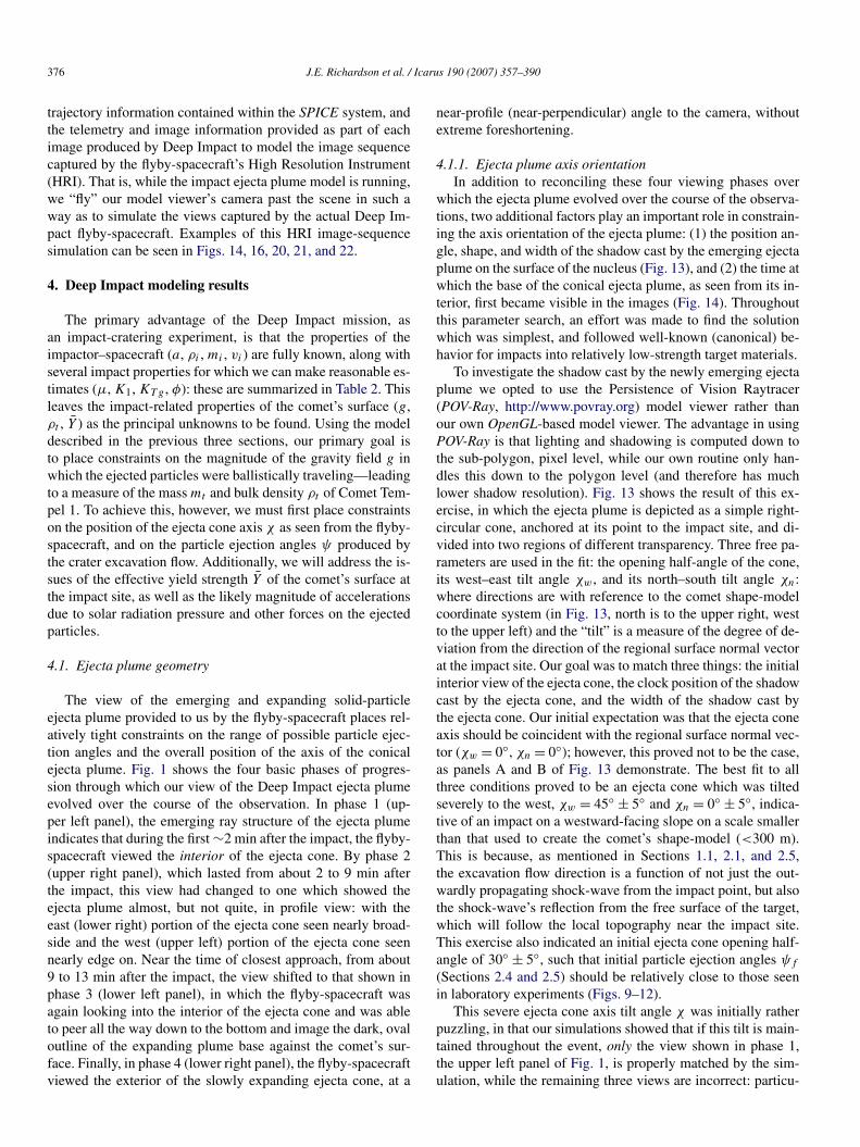
376 J.E. Richardson et al. / Icarus 190 (2007) 357–390
trajectory information contained within the SPICE system, andthe telemetry and image information provided as part of eachimage produced by Deep Impact to model the image sequencecaptured by the flyby-spacecraft’s High Resolution Instrument(HRI). That is, while the impact ejecta plume model is running,we “fly” our model viewer’s camera past the scene in such away as to simulate the views captured by the actual Deep Im-pact flyby-spacecraft. Examples of this HRI image-sequencesimulation can be seen in Figs. 14, 16, 20, 21, and 22.
4. Deep Impact modeling results
The primary advantage of the Deep Impact mission, asan impact-cratering experiment, is that the properties of theimpactor–spacecraft (a, ρi , mi , vi ) are fully known, along withseveral impact properties for which we can make reasonable es-timates (μ, K1, KTg , φ): these are summarized in Table 2. Thisleaves the impact-related properties of the comet’s surface (g,ρt , Y ) as the principal unknowns to be found. Using the modeldescribed in the previous three sections, our primary goal isto place constraints on the magnitude of the gravity field g inwhich the ejected particles were ballistically traveling—leadingto a measure of the mass mt and bulk density ρt of Comet Tem-pel 1. To achieve this, however, we must first place constraintson the position of the ejecta cone axis χ as seen from the flyby-spacecraft, and on the particle ejection angles ψ produced bythe crater excavation flow. Additionally, we will address the is-sues of the effective yield strength Y of the comet’s surface atthe impact site, as well as the likely magnitude of accelerationsdue to solar radiation pressure and other forces on the ejectedparticles.
4.1. Ejecta plume geometry
The view of the emerging and expanding solid-particleejecta plume provided to us by the flyby-spacecraft places rel-atively tight constraints on the range of possible particle ejec-tion angles and the overall position of the axis of the conicalejecta plume. Fig. 1 shows the four basic phases of progres-sion through which our view of the Deep Impact ejecta plumeevolved over the course of the observation. In phase 1 (up-per left panel), the emerging ray structure of the ejecta plumeindicates that during the first ∼2 min after the impact, the flyby-spacecraft viewed the interior of the ejecta cone. By phase 2(upper right panel), which lasted from about 2 to 9 min afterthe impact, this view had changed to one which showed theejecta plume almost, but not quite, in profile view: with theeast (lower right) portion of the ejecta cone seen nearly broad-side and the west (upper left) portion of the ejecta cone seennearly edge on. Near the time of closest approach, from about9 to 13 min after the impact, the view shifted to that shown inphase 3 (lower left panel), in which the flyby-spacecraft wasagain looking into the interior of the ejecta cone and was ableto peer all the way down to the bottom and image the dark, ovaloutline of the expanding plume base against the comet’s sur-face. Finally, in phase 4 (lower right panel), the flyby-spacecraftviewed the exterior of the slowly expanding ejecta cone, at a
near-profile (near-perpendicular) angle to the camera, withoutextreme foreshortening.
4.1.1. Ejecta plume axis orientationIn addition to reconciling these four viewing phases over
which the ejecta plume evolved over the course of the observa-tions, two additional factors play an important role in constrain-ing the axis orientation of the ejecta plume: (1) the position an-gle, shape, and width of the shadow cast by the emerging ejectaplume on the surface of the nucleus (Fig. 13), and (2) the time atwhich the base of the conical ejecta plume, as seen from its in-terior, first became visible in the images (Fig. 14). Throughoutthis parameter search, an effort was made to find the solutionwhich was simplest, and followed well-known (canonical) be-havior for impacts into relatively low-strength target materials.
To investigate the shadow cast by the newly emerging ejectaplume we opted to use the Persistence of Vision Raytracer(POV-Ray, http://www.povray.org) model viewer rather thanour own OpenGL-based model viewer. The advantage in usingPOV-Ray is that lighting and shadowing is computed down tothe sub-polygon, pixel level, while our own routine only han-dles this down to the polygon level (and therefore has muchlower shadow resolution). Fig. 13 shows the result of this ex-ercise, in which the ejecta plume is depicted as a simple right-circular cone, anchored at its point to the impact site, and di-vided into two regions of different transparency. Three free pa-rameters are used in the fit: the opening half-angle of the cone,its west–east tilt angle χw , and its north–south tilt angle χn:where directions are with reference to the comet shape-modelcoordinate system (in Fig. 13, north is to the upper right, westto the upper left) and the “tilt” is a measure of the degree of de-viation from the direction of the regional surface normal vectorat the impact site. Our goal was to match three things: the initialinterior view of the ejecta cone, the clock position of the shadowcast by the ejecta cone, and the width of the shadow cast bythe ejecta cone. Our initial expectation was that the ejecta coneaxis should be coincident with the regional surface normal vec-tor (χw = 0◦, χn = 0◦); however, this proved not to be the case,as panels A and B of Fig. 13 demonstrate. The best fit to allthree conditions proved to be an ejecta cone which was tiltedseverely to the west, χw = 45◦ ± 5◦ and χn = 0◦ ± 5◦, indica-tive of an impact on a westward-facing slope on a scale smallerthan that used to create the comet’s shape-model (<300 m).This is because, as mentioned in Sections 1.1, 2.1, and 2.5,the excavation flow direction is a function of not just the out-wardly propagating shock-wave from the impact point, but alsothe shock-wave’s reflection from the free surface of the target,which will follow the local topography near the impact site.This exercise also indicated an initial ejecta cone opening half-angle of 30◦ ± 5◦, such that initial particle ejection angles ψf
(Sections 2.4 and 2.5) should be relatively close to those seenin laboratory experiments (Figs. 9–12).
This severe ejecta cone axis tilt angle χ was initially ratherpuzzling, in that our simulations showed that if this tilt is main-tained throughout the event, only the view shown in phase 1,the upper left panel of Fig. 1, is properly matched by the sim-ulation, while the remaining three views are incorrect: particu-
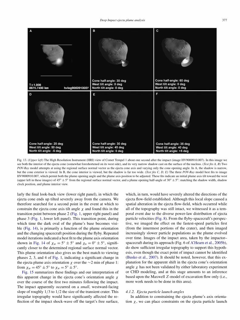
Deep Impact ejecta plume analysis 377
Fig. 13. (Upper left) The High Resolution Instrument (HRI) view of Comet Tempel 1 about one second after the impact (image HV9000910.007). In this image wesee both the interior of the ejecta cone (somewhat foreshortened on its west side), and its very narrow shadow cast on the surface of the nucleus. (Test fits A, B) TwoPOV-Ray model attempts at using the regional surface normal vector as the ejecta cone axis and varying only the cone opening angle. In A, the shadow is narrow,but the cone exterior is viewed. In B, the cone interior is viewed, but the shadow is far too wide. (Test fits C, D, E) The three POV-Ray model best fits to imageHV9000910.007, which permit both the plume opening angle and the plume axis position to be adjusted. These fits indicate an initial plume axis tilt toward the west(upper left in these images) of 45◦ ± 5◦ from the regional surface normal vector, and a plume opening half-angle of 30◦ ± 5◦: matching the shadow width, shadowclock position, and plume interior view.
larly the final look-back view (lower right panel), in which theejecta cone ends up tilted severely away from the camera. Wetherefore searched for a second point in the event at which toconstrain the ejecta cone axis tilt angle χ and found this in thetransition point between phase 2 (Fig. 1, upper right panel) andphase 3 (Fig. 1, lower left panel). This transition point, duringwhich time the dark oval of the plume’s base becomes visi-ble (Fig. 14), is primarily a function of the plume orientationand the changing spacecraft position during the flyby. Repeatedmodel iterations indicated a best fit to the plume axis orientationshown in Fig. 14 of χw = 5◦ ± 5◦ and χn = 0◦ ± 5◦, signifi-cantly closer to the determined regional surface normal vector.This plume orientation also gives us the best match to viewingphases 2, 3, and 4 of Fig. 1, indicating a significant change inthe ejecta plume axis orientation χ over the ∼2 min of phase 1:from χw = 45◦ ± 5◦ to χw = 5◦ ± 5◦.
Fig. 15 summarizes these findings and our interpretation ofthis apparent change in the ejecta cone’s orientation angle χ
over the course of the first two minutes following the impact.The impact apparently occurred on a small, westward-facingslope of roughly 1/3 to 1/2 the size of the transient crater. Thisirregular topography would have significantly affected the re-flection of the impact shock-wave off the target’s free surface,
which, in turn, would have severely altered the directions of theejecta flow-field established. Although this local slope caused aspatial alteration in the ejecta flow-field, which occurred whileall of the topography was still intact, we witnessed it as a tem-poral event due to the diverse power-law distribution of ejectaparticle velocities (Fig. 8). From the flyby-spacecraft’s perspec-tive, we imaged the effect on the fastest-speed particles first(from the innermost portions of the crater), and then imagedincreasingly slower particle populations as the plume evolvedover time. Images of the impact area, taken by the impactor–spacecraft during its approach (Fig. 6 of A’Hearn et al., 2005b),do show sufficient irregular topography to support this hypoth-esis, even though the exact point of impact cannot be identified(Busko et al., 2007). It should be noted, however, that this ex-planation for the apparent shift in the ejecta cone’s orientationangle χ has not been validated by either laboratory experimentor CHD modeling, and at this stage amounts to an inferencebased upon the Maxwell Z-model of excavation flow only (i.e.,more work needs to be done in this area).
4.1.2. Ejecta particle launch anglesIn addition to constraining the ejecta plume’s axis orienta-
tion χ , we can place constraints on the ejecta particle launch
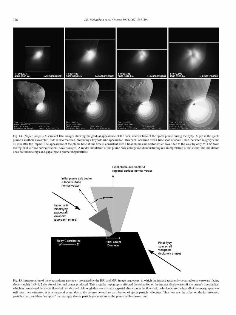
378 J.E. Richardson et al. / Icarus 190 (2007) 357–390
Fig. 14. (Upper images) A series of HRI images showing the gradual appearance of the dark, interior base of the ejecta plume during the flyby. A gap in the ejectaplume’s southern (lower left) side is also revealed, producing a keyhole-like appearance. This event occurred over a time span of about 1 min, between roughly 9 and10 min after the impact. The appearance of the plume base at this time is consistent with a final plume axis vector which was tilted to the west by only 5◦ ± 5◦ fromthe regional surface normal vector. (Lower images) A model simulation of the plume base emergence, demonstrating our interpretation of the event. The simulationdoes not include rays and gaps (ejecta plume irregularities).
Fig. 15. Interpretation of the ejecta plume geometry presented by the HRI and MRI image sequences, in which the impact apparently occurred on a westward-facingslope roughly 1/3–1/2 the size of the final crater produced. This irregular topography affected the reflection of the impact shock-wave off the target’s free surface,which in turn altered the ejecta flow-field established. Although this was actually a spatial alteration in the flow-field, which occurred while all of the topography wasstill intact, we witnessed it as a temporal event, due to the diverse power-law distribution of ejecta particle velocities. Thus, we saw the affect on the fastest-speedparticles first, and then “sampled” increasingly slower particle populations as the plume evolved over time.

Deep Impact ejecta plume analysis 379
Fig. 16. A series of model simulations used to fit the ejecta plume side angles shown in image HV9010003.001, by varying the parameters of ψn (Eq. (44)) in suchas way as to keep the mean ejection angle at ψ ≈ 45◦ . Although the boundaries of the actual ejecta plume are somewhat diffuse, a reasonable fit is achieved atstarting angles of ψo = 60◦ ± 5◦ and a total angular drop of ψd = 30◦ ± 10◦ .
angles ψ . As mentioned earlier, the HRI image of the newlyemerging plume (Fig. 13) is best modeled by an ejecta coneopening angle which is consistent with experimentally pro-duced ejecta plumes (Cintala et al., 1999; Anderson et al.,2003, 2004). To further constrain this, we took advantage ofthe near-profile view of the ejecta plume afforded by the firstlook-back images (phase 4). As shown in Fig. 16, repeatedmodel iterations indicated that the most straight-forward wayto fit the ejecta plume side positions was achieved by vary-ing the parameters of ψn (Eq. (44)) in such as way as to keepthe mean ejection angle at ψ ≈ 45◦. Although the boundariesof the actual ejecta plume are somewhat diffuse, a reasonablefit is achieved at starting angles of ψo = 60◦ ± 5◦ and totalangular drops of ψd = 30◦ ± 10◦. There are two reasons forkeeping the mean ejection angle at ψ ≈ 45◦: first, it keepsour model consistent with experimental findings, in which ψ
is generally within the range of 40◦–45◦ (Section 2.4); andsecond, it keeps our model consistent with our ejecta veloc-ity constant derivation assumptions (Section 2.2) and those ofthe original Maxwell Z-model (Maxwell and Seifert, 1974;Maxwell, 1977). It should be noted, however, that our solu-tion is non-unique, and we have therefore selected the solutionwhich is most consistent with past experiments and our currentmodel derivation.
4.2. Tempel 1 gravity and bulk density
With the ejecta plume axis orientation χ and particle ejec-tion angles ψ reasonably constrained, the next phase of theanalysis was to determine the magnitude of the gravity fieldin which these particles were ballistically traveling (a functionof the comet’s bulk density). During the excavation and falloutphases of an impact event, the ejecta plume forms an inverted,hollow cone, and marks the position locus of the solid ejectaparticles in flight at that time (Fig. 11): its bottom region iscomposed of particles nearing the end of their flight and fallingout of the plume; its middle region is composed of particlesmidway through their ballistic flight and traveling nearly radialto the ejecta cone’s axis; and its upper region is composed ofparticles which have not yet reached the apex of their ballisticflights, with the uppermost particles traveling faster than the es-cape velocity of the comet and therefore never returning to thesurface. Because each ejecta particle is following its own bal-listic trajectory under the influence of Tempel 1’s gravity field,the lateral expansion rate of the collective ejecta plume is alsoa function of the comet’s gravity field (Melosh, 2001).
To measure the lateral expansion rate of the ejecta plumeproduced by Deep Impact, we use the plume’s base as our com-mon point of reference and monitor the plume base diameteras a function of time. Fig. 17 shows several model examples
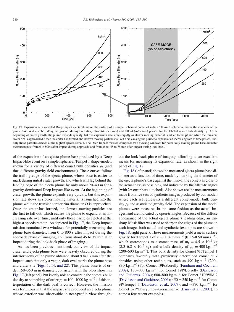
380 J.E. Richardson et al. / Icarus 190 (2007) 357–390
Fig. 17. Expansion of a modeled Deep Impact ejecta plume on the surface of a simple, spherical comet of radius 3.0 km. Each curve marks the diameter of theplume base as it marches along the ground, during both its ejection (dashed line) and fallout (solid line) phases, for the labeled comet bulk density ρt . At thebeginning of crater growth, the plume expands quickly, but this expansion rate slows rapidly as slower moving material is added to the plume while the transientcrater rim is approached. Once the crater has formed, the slowest moving particles fall out first, causing the plume to expand at an increasing rate as time passes, untilonly those particles ejected at the highest speeds remain. The Deep Impact mission comprised two viewing windows for potentially making plume base diametermeasurements: from 0 to 800 s after impact during approach, and from about 45 to 75 min after impact during look-back.
of the expansion of an ejecta plume base produced by a DeepImpact-like event on a simple, spherical Tempel 1 shape-model,shown for a variety of different comet bulk densities ρt (andthus different gravity field environments). These curves followthe trailing edge of the ejecta plume, whose base is easier tomark during initial crater growth, and which will lag behind theleading edge of the ejecta plume by only about 20–40 m for agravity-dominated Deep Impact-like event. At the beginning ofcrater growth, the plume expands very quickly, but this expan-sion rate slows as slower moving material is launched into theplume while the transient crater rim diameter D is approached.Once the crater has formed, the slowest moving particles arethe first to fall out, which causes the plume to expand at an in-creasing rate over time, until only those particles ejected at thehighest speeds remain. As depicted in Fig. 17, the Deep Impactmission contained two windows for potentially measuring theplume base diameter: from 0 to 800 s after impact during theapproach phase of imaging, and from about 45 to 75 min afterimpact during the look-back phase of imaging.
As has been previous mentioned, our view of the impactcrater and ejecta plume base were heavily obscured during theinterior views of the plume obtained about 9 to 13 min after theimpact, such that only a vague, dark oval marks the plume baseand crater site (Figs. 1, 14, and 22). This plume base is of or-der 150–350 m in diameter, consistent with the plots shown inFig. 17 (left panel), but is only able to constrain the comet’s bulkdensity to something of order ρt = 100–1000 kg m−3, if this in-terpretation of the dark oval is correct. However, the missionwas fortuitous in that the impact site produced an ejecta plumewhose exterior was observable in near-profile view through-
out the look-back phase of imaging, affording us an excellentmeans for measuring its expansion rate, as shown in the rightpanel of Fig. 17.
Fig. 18 (left panel) shows the measured ejecta plume base di-ameter as a function of time, made by marking the diameter ofthe ejecta plume’s base against the limb of the comet (as close tothe actual base as possible), and indicated by the filled-triangles(with 2σ error bars attached). Also shown are the measurementsmade from five sets of synthetic images produced by our model,where each set represents a different comet-model bulk den-sity ρt and associated gravity field. The expansion of the modelplumes were measured in the same fashion as the actual im-ages, and are indicated by open-triangles. Because of the diffuseappearance of the actual ejecta plume’s leading edge, an Un-sharp Mask filter was used to sharpen the edges of the plume ineach image, both actual and synthetic (examples are shown inFig. 18, right panel). These measurements yield a mean surfacegravity for Tempel 1 of g = 0.34 mm s−2 (0.17–0.50 mm s−2),which corresponds to a comet mass of mt = 4.5 × 10¹³ kg(2.3–6.8 × 10¹³ kg) and a bulk density of ρt = 400 kg m−3
(200–600 kg m−3). This bulk density for Comet 9P/Tempel 1compares favorably with previously determined comet bulkdensities using other techniques, such as 490 kg m−3 (290–830 kg m−3) for Comet 19P/Borrelly (Farnham and Cochran,2002); 180–300 kg m−3 for Comet 19P/Borrelly (Davidssonand Gutiérrez, 2004); 600–800 kg m−3 for Comet 81P/Wild 2(Davidsson and Gutiérrez, 2006); 450 ± 250 kg m−3 for Comet9P/Tempel 1 (Davidsson et al., 2007); and ∼370 kg m−3 forComet 67P/Churyumov–Gerasimenko (Lamy et al., 2007), toname a few recent examples.

Deep Impact ejecta plume analysis 381
Fig. 18. (Left) Expansion of the actual Deep Impact ejecta plume, measured by marking the diameter of the plume base against the limb of the comet during thelook-back phase of imaging. Filled black triangles are measurements from the actual images (HV9010003.001–HV9010052.001), shown with 2σ error bars. Opentriangles are measurements made from model-produced synthetic images, at five different comet-model bulk densities ρt . Each set of measurements is connectingusing a least-squares polynomial fit, the dotted line for the actual image measurements and the solid lines for the synthetic image measurements, with a verygood match occurring at a model bulk density of ρt = 400 kg m−3 (200–600 kg m−3). (Right) Four examples of the images used to create this plot, as shown inedge-sharpened, re-scaled actual images (upper) and synthetic model images (lower). The left-hand images are from the beginning of the look-back phase (45 minafter impact), while the right-hand images are from the end of the look-back phase (75 min after impact).
Although the agreement of our results with these previousestimates is good, all of these estimates are based on the com-putation of non-gravitational forces for the various cometarynuclei, computations that involve many assumptions and aregenerally regarded as very uncertain (Weissman et al., 2004).Because all spacecraft encounters with comets to date, includ-ing Deep Impact, have been fast flybys at distances of manynuclear radii, it has not been possible to compute the massdirectly from the deflection of the spacecraft. Other methods,such as modeling the unique tidal breakup of Comet SL/9, re-lations between the rotation period and shape of comet nuclei,and estimates from the density of cometary dust particles plusassumptions about how comets are assembled all yield similar,but also uncertain density estimates (Weissman et al., 2004).Our method of modeling ejecta plume expansion is differentthan previous methods, but it suffers similarly from many un-certainties, as explained in this paper. Before the Deep Impactencounter with Tempel 1 we had anticipated the ability to trackdiscrete boulders ejected from the impact (Richardson et al.,2005). Indeed, the image sequence we adopted, particularly thelook-back imaging, was planned with the expectation of beingable to track ballistically ejected boulders and thus get goodestimates of the gravitational acceleration near Tempel 1’s nu-cleus. Modeling the ejecta plume expansion to determine grav-ity was regarded as a “last-ditch” option that we hoped wewould not have to exercise, but we developed it in case all elsefailed. As events turned out, however, boulders were not de-tected in the ejecta plume, nor did we see coherent boulderson the surface of Tempel 1 at our highest resolution. While
this observation has important consequences for the geology ofTempel 1, it is an unfortunate circumstance for gravity determi-nation. Nevertheless, our careful modeling of the ejecta plumehas yielded useful constrains on the density of Tempel 1 thatare completely independent of other methods of density deter-mination.
There are four potential sources for error in this comet den-sity estimate: image measurement errors (shown in Fig. 18),comet shape-model errors (Thomas et al., 2007), ejecta plumemodel errors (this work), and non-gravitational forces (Sec-tion 4.4). The rather diffuse plume edge appearance in the HRIlook-back images meant that different amounts of edge sharp-ening change the apparent plume width slightly: creating up toa 50% fractional error in the density measurement (2σ ). Thecomet shape-model from Thomas et al. (2007), with a mean ra-dius of 3.0±0.1 km, has a volume error of 10%, but in terms ofthe density (which goes as 1/radius) this produces a fractionalerror of only 3.3% in the density measurement. Model-plumewidth variations in the synthetic images, created by exercisingour model parameters over their full ranges (Tables 2 and 4),produce up to a 10% fractional error in the density measure-ment. Combining all three quantified sources of error yields atotal fractional error of 51% in the density measurement, suchthat the measurement errors from the HRI look-back imagescompletely outweigh the other potential sources discussed here.The effects of non-gravitational forces on the ejecta plume ex-pansion rate, however, are more difficult to quantify, with thepotential effect of coma gas pressure being the most problem-atic. This will be discussed further in Section 4.4.
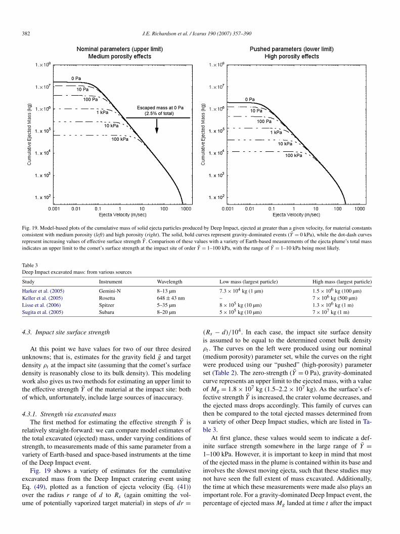
382 J.E. Richardson et al. / Icarus 190 (2007) 357–390
Fig. 19. Model-based plots of the cumulative mass of solid ejecta particles produced by Deep Impact, ejected at greater than a given velocity, for material constantsconsistent with medium porosity (left) and high porosity (right). The solid, bold curves represent gravity-dominated events (Y = 0 kPa), while the dot-dash curvesrepresent increasing values of effective surface strength Y . Comparison of these values with a variety of Earth-based measurements of the ejecta plume’s total massindicates an upper limit to the comet’s surface strength at the impact site of order Y = 1–100 kPa, with the range of Y = 1–10 kPa being most likely.
Table 3Deep Impact excavated mass: from various sources
Study Instrument Wavelength Low mass (largest particle) High mass (largest particle)
Harker et al. (2005) Gemini-N 8–13 µm 7.3 × 10⁴ kg (1 µm) 1.5 × 10⁶ kg (100 µm)Keller et al. (2005) Rosetta 648 ± 43 nm – 7 × 10⁶ kg (500 µm)Lisse et al. (2006) Spitzer 5–35 µm 8 × 10⁵ kg (10 µm) 1.3 × 10⁶ kg (1 m)Sugita et al. (2005) Subaru 8–20 µm 5 × 10⁵ kg (10 µm) 7 × 10⁷ kg (1 m)
4.3. Impact site surface strength
At this point we have values for two of our three desiredunknowns; that is, estimates for the gravity field g and targetdensity ρt at the impact site (assuming that the comet’s surfacedensity is reasonably close to its bulk density). This modelingwork also gives us two methods for estimating an upper limit tothe effective strength Y of the material at the impact site: bothof which, unfortunately, include large sources of inaccuracy.
4.3.1. Strength via excavated massThe first method for estimating the effective strength Y is
relatively straight-forward: we can compare model estimates ofthe total excavated (ejected) mass, under varying conditions ofstrength, to measurements made of this same parameter from avariety of Earth-based and space-based instruments at the timeof the Deep Impact event.
Fig. 19 shows a variety of estimates for the cumulativeexcavated mass from the Deep Impact cratering event usingEq. (49), plotted as a function of ejecta velocity (Eq. (41))over the radius r range of d to Rs (again omitting the vol-ume of potentially vaporized target material) in steps of dr =
(Rs − d)/104. In each case, the impact site surface densityis assumed to be equal to the determined comet bulk densityρt . The curves on the left were produced using our nominal(medium porosity) parameter set, while the curves on the rightwere produced using our “pushed” (high-porosity) parameterset (Table 2). The zero-strength (Y = 0 Pa), gravity-dominatedcurve represents an upper limit to the ejected mass, with a valueof Mg = 1.8 × 10⁷ kg (1.5–2.2 × 10⁷ kg). As the surface’s ef-fective strength Y is increased, the crater volume decreases, andthe ejected mass drops accordingly. This family of curves canthen be compared to the total ejected masses determined froma variety of other Deep Impact studies, which are listed in Ta-ble 3.
At first glance, these values would seem to indicate a def-inite surface strength somewhere in the large range of Y =1–100 kPa. However, it is important to keep in mind that mostof the ejected mass in the plume is contained within its base andinvolves the slowest moving ejecta, such that these studies maynot have seen the full extent of mass excavated. Additionally,the time at which these measurements were made also plays animportant role. For a gravity-dominated Deep Impact event, thepercentage of ejected mass Mg landed at time t after the impact
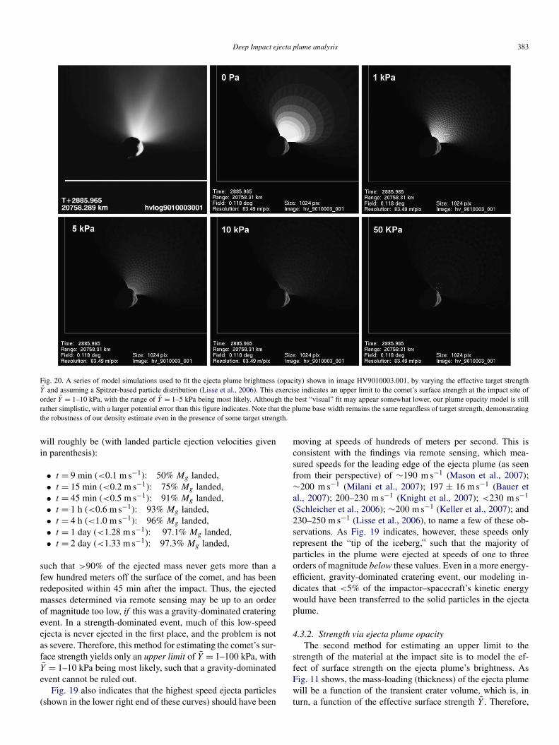
Deep Impact ejecta plume analysis 383
Fig. 20. A series of model simulations used to fit the ejecta plume brightness (opacity) shown in image HV9010003.001, by varying the effective target strengthY and assuming a Spitzer-based particle distribution (Lisse et al., 2006). This exercise indicates an upper limit to the comet’s surface strength at the impact site oforder Y = 1–10 kPa, with the range of Y = 1–5 kPa being most likely. Although the best “visual” fit may appear somewhat lower, our plume opacity model is stillrather simplistic, with a larger potential error than this figure indicates. Note that the plume base width remains the same regardless of target strength, demonstratingthe robustness of our density estimate even in the presence of some target strength.
will roughly be (with landed particle ejection velocities givenin parenthesis):
• t = 9 min (<0.1 m s−1): 50% Mg landed,• t = 15 min (<0.2 m s−1): 75% Mg landed,• t = 45 min (<0.5 m s−1): 91% Mg landed,• t = 1 h (<0.6 m s−1): 93% Mg landed,• t = 4 h (<1.0 m s−1): 96% Mg landed,• t = 1 day (<1.28 m s−1): 97.1% Mg landed,• t = 2 day (<1.33 m s−1): 97.3% Mg landed,
such that >90% of the ejected mass never gets more than afew hundred meters off the surface of the comet, and has beenredeposited within 45 min after the impact. Thus, the ejectedmasses determined via remote sensing may be up to an orderof magnitude too low, if this was a gravity-dominated crateringevent. In a strength-dominated event, much of this low-speedejecta is never ejected in the first place, and the problem is notas severe. Therefore, this method for estimating the comet’s sur-face strength yields only an upper limit of Y = 1–100 kPa, withY = 1–10 kPa being most likely, such that a gravity-dominatedevent cannot be ruled out.
Fig. 19 also indicates that the highest speed ejecta particles(shown in the lower right end of these curves) should have been
moving at speeds of hundreds of meters per second. This isconsistent with the findings via remote sensing, which mea-sured speeds for the leading edge of the ejecta plume (as seenfrom their perspective) of ∼190 m s−1 (Mason et al., 2007);∼200 m s−1 (Milani et al., 2007); 197 ± 16 m s−1 (Bauer etal., 2007); 200–230 m s−1 (Knight et al., 2007); <230 m s−1
(Schleicher et al., 2006); ∼200 m s−1 (Keller et al., 2007); and230–250 m s−1 (Lisse et al., 2006), to name a few of these ob-servations. As Fig. 19 indicates, however, these speeds onlyrepresent the “tip of the iceberg,” such that the majority ofparticles in the plume were ejected at speeds of one to threeorders of magnitude below these values. Even in a more energy-efficient, gravity-dominated cratering event, our modeling in-dicates that <5% of the impactor–spacecraft’s kinetic energywould have been transferred to the solid particles in the ejectaplume.
4.3.2. Strength via ejecta plume opacityThe second method for estimating an upper limit to the
strength of the material at the impact site is to model the ef-fect of surface strength on the ejecta plume’s brightness. AsFig. 11 shows, the mass-loading (thickness) of the ejecta plumewill be a function of the transient crater volume, which is, inturn, a function of the effective surface strength Y . Therefore,

384 J.E. Richardson et al. / Icarus 190 (2007) 357–390
Table 4Model determined parameters
Name Symbol Nominal value Value range
Initial plume axis N–S tilt χno 0◦ ±5◦Initial plume axis W–E tilt χwo 45◦ ±5◦Final plume axis N–S tilt χnf 0◦ ±5◦Final plume axis W–E tilt χwf 5◦ ±5◦Initial particle ejection angle ψo 60◦ ±5◦Particle ejection angle drop ψd 30◦ ±10◦Impact site surface strength Y 0–5 kPa 0–10 kPaTempel 1 mean gravity g 0.34 mm s−2 0.17–0.90 mm s−2
Tempel 1 bulk density ρt 400 kg m−3 200–1000 kg m−3
Tempel 1 mass mt 4.5 × 10¹³ kg 2.3–12.0 × 10¹³ kg
Crater diameter (Y = 0 Pa) Dg 100 m 85–140 mCrater formation time(Y = 0 Pa)
Tg 330 s 250–550 s
Crater excavated mass(Y = 0 Pa)
Mg 1.8 × 10⁷ kg 1.5–2.2 × 10⁷ kg
Crater diameter (Y = 1 kPa) Ds 37 m 35–41 mCrater formation time(Y = 1 kPa)
Ts 11 s 8–12 s
Crater excavated mass(Y = 1 kPa)
Ms 0.91 × 10⁶ kg 0.60–1.2 × 10⁶ kg
Crater diameter (Y = 10 kPa) Ds 24 m 22–26 mCrater formation time(Y = 10 kPa)
Ts 2 s 1–3 s
Crater excavated mass(Y = 10 kPa)
Ms 2.3 × 10⁵ kg 1.5–2.9 × 10⁵ kg
we can use the opacity of the ejecta plume (Eq. (56)) as a meansto gauge its mass-loading, provided that we have an indepen-dent means for determining the ejecta particle size distribution(PSD).
Fig. 20 shows a comparison between the first look-back im-age obtained by the HRI instrument and several model runs ofvarying effective surface strength Y . Each of these syntheticimages uses the particle size distribution (PSD) determined viathe space-based Spitzer telescope (Lisse et al., 2006), whichuses an ejecta particle size range of 0.1 to at least 20 µm,with a peak at 1.0 µm. We have also assumed an individualparticle density of ρp = 1750 kg m−3: a 50% mixture of iceand silicate dust (Sunshine et al., 2007). These synthetic im-age comparisons place an upper limit on the comet’s surfacestrength at the impact site of Y = 1–10 kPa, with the rangeof Y = 1–5 kPa being most likely; where again, a gravity-dominated event cannot be ruled out. This strength determina-tion is consistent with the estimate from the cumulative exca-vated mass model (Section 4.3.1), and the strength determinedby Holsapple and Housen (2007). Note that although the best“visual” fit occurs in the top images of Fig. 20, for Y values ofup to 1 kPa, our current ejecta plume opacity model is some-what simplistic (Section 3.2), and the potential error remainslarge at this point.
4.4. The effects of non-gravitational forces
Up to this point, the ejecta ballistics model has containedonly the acceleration due to gravity g as an external force act-
ing on the ejecta particles once they are launched. However,because Deep Impact occurred on a cometary nucleus, and pro-duced an ejecta plume composed of very fine particles, thereare five potential sources for additional forces on the ejectaparticles in flight which need to be considered, especially withregard to their potential effect on the Tempel 1 gravity and bulkdensity estimate (Section 4.2). Two of these potential sources,solar radiation pressure and coma gas pressure, are inherent tothe cometary environment in which the impact took place. Theremaining three potential sources were produced by the im-pact event itself: the initial vapor plume, water-gas sublimationfrom icy grains within the ejecta plume, and impact-inducedcometary activity following the cratering event.
4.4.1. Solar radiation pressureSolar radiation pressure will show its effect as an accelera-
tion in the anti-solar direction, affecting all insolated ejecta par-ticles proportional to their (surface area) × (photon absorption-scattering efficiency)/(mass) product. The most pronounced ef-fect will be on small particles with sizes 0.1–1.0 µm, whichhave very little mass but possess high scattering efficiency dueto a similar size to the wavelengths of visual light. The rela-tive effect of solar radiation pressure is usually expressed incomparison to the force of solar gravity at the comet’s loca-tion: β = FRadiation pressure/FSolar gravity. Beta is also related tothe surface/volume ratio of a dust particle, since the radiationpressure force depends on the surface area of the particle ab-sorbing sunlight, while the gravitational force depends on theparticle’s volume. Typical values of Beta are ∼1 for particles of0.5–1.5 µm in radius, falling off inversely with radius for largerparticles, and typical time scales for the importance of this ef-fect in cometary dust comae and tails at 1 AU is on the order ofdays to weeks (Lisse et al., 1998). Since the measured Deep Im-pact ejecta size distribution consisted of a majority of particlesof this size (Lisse et al., 2006), we expect this to be an impor-tant force, but since the timescale over which the observationswere made was short, 1/50th to 1/500th the typical amount oftime, the overall effect may not be very large.
In examining the Deep Impact HRI images, we do find in-dications of a small, anti-solar drift in the ejecta plume baseby the time of the first look-back images, when compared tomodel-produced synthetic images (Figs. 18 and 20). This driftis not more than about 400–800 m, which corresponds to an ac-celeration of 0.1–0.2 mm s−2 in the anti-solar direction. Notehowever, that this motion appears to involve all particles in theejecta plume, such that the entire plume is slightly displaced,and thus the ejecta cone’s expansion rate (used in the gravityestimate) is not affected. Additional model iterations were per-formed which included this apparent acceleration (Section 3.3),and although there are small measurement changes due to themodel plume being located behind a slightly different portionof the comet’s limb, these changes do not effect the overall ex-pansion rate or best-fit gravity/density solution.
The observed small drift in ejecta plume position can, how-ever, be used to estimate the mean particle size in the ejectaplume at the time of the look-back observations. At the distanceof Tempel 1 from the sun at the time of encounter, an anti-solar
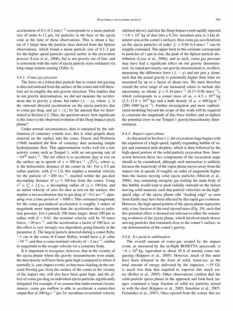
Deep Impact ejecta plume analysis 385
acceleration of 0.1–0.2 mm s−2 corresponds to a mean particlesize of order 6–12 µm, for particles in the base of the ejectacone at the time of these observations. This is about a fac-tor of 3 larger than the particle sizes derived from the Spitzerobservations, which found a mean particle size of 0.1–2 µmfor the higher speed particles ejected earlier in the excavationprocess (Lisse et al., 2006), but is not grossly out of line, andis consistent with the suite of ejecta particle sizes estimated vialong-range remote sensing (Table 3).
4.4.2. Coma gas pressureThe force on a lofted dust particle due to comet out-gassing
is directed outward from the surface of the comet and will there-fore act in roughly the anti-gravity direction. This implies thatin our gravity determination, we did not measure the acceler-ation due to gravity g alone, but rather (fc − g), where fc isthe outward directed acceleration on the ejecta particles dueto coma gas drag, and |g| > |fc| by the amount that we deter-mined in Section 4.2. Thus, the question arises: how significantis this force to the observed evolution of the Deep Impact ejectaplume?
Under normal circumstances, dust is entrained by the sub-limation of cometary volatile ices: this is what propels dustymaterial on the surface into the coma. Finson and Probstein(1968) modeled the flow of cometary dust assuming simplehydrodynamic flow. This approximation works well for a lowactivity comet such as Tempel 1, with an out-gassing rate of∼1028 mol s−1. The net effect is to accelerate dust at rest onthe surface up to speeds of v = 300 m s−1 √
β/rh, where rhis the heliocentric distance of the comet in AU. For a 0.5 µmradius particle, with β ≈ 1.0, this implies a terminal velocityfor the particle of ∼200 m s−1, reached within the gas-dustdecoupling distance of rd ≈ 100 km from the comet. Usingv2 = v2
o + 2fcrd , a decoupling radius of rd = 100 km, andan initial velocity of zero for dust at rest on the surface, thisimplies a net acceleration due to gas drag of ∼0.2 m s−2, oper-ating over a time period of ∼1000 s. This estimated magnitudefor the coma gas-induced acceleration is roughly 3 orders ofmagnitude more important than the acceleration due to radia-tion pressure. For a particle 100 times larger, about 100 µm inradius with β ∼ 0.01, the terminal velocity will be 10 timeslower, ∼20 m s−1, and the acceleration a factor of 100 less: sothis effect is very strongly size dependent, going linearly in theparameter β . The largest particle detected during a comet flyby,∼1 cm in the coma of Comet Halley, would have a β value∼10−4, and thus a coma terminal velocity of ∼2 m s−1, similarin magnitude to the escape velocity for a cometary body.
It is important to recognize, however, that in the vicinity ofthe ejecta plume where the gravity measurements were made,the dust density will have been quite high (compared to where itnormally is, sans impact event), so that mass-loading on the out-ward flowing gas, from the surface of the comet in the vicinityof the impact site, will also have been quite high, and the af-fect of coma gas drag on individual ejecta particles significantlymitigated. For example, if we assume that under normal circum-stances, coma gas outflow is able to accelerate a comet-dustoutput flux of 200 kg s−1 per 2π steradians to terminal velocity
(defined above), and that the Deep Impact event rapidly injected∼1.0 × 10⁷ kg of dust into a 0.24π steradian area (a 3 km di-ameter area at the comet’s surface), then coma gas accelerationson the ejecta particles of order fc = 0.04–0.4 mm s−2 can beroughly estimated. The upper limit in this estimate correspondsto particles of 1 µm in size, the peak of the Spitzer particle dis-tribution (Lisse et al., 2006), and as such, coma gas pressuremay have had a significant effect on our gravity determina-tion. As stated previously, our gravity measurement is, in effect,measuring the difference force (fc − g) and not just g alone,such that the actual gravity is potentially higher than what wemeasured by up to a factor of about two. We must thereforeextend the error range of our measured values to include thisuncertainty, to obtain: g = 0.34 mm s−2 (0.17–0.90 mm s−2),which corresponds to a comet mass of mt = 4.5 × 10¹³ kg(2.3–12.0 × 10¹³ kg) and a bulk density of ρt = 400 kg m−3
(200–1000 kg m−3). Further investigation and more sophisti-cated modeling beyond the scope of this work will be requiredto constrain the magnitude of this force further, and re-tightenthe potential error in our Tempel 1 gravity/mass/density deter-mination.
4.4.3. Impact vapor plumeAs discussed in Section 1.1, the excavation stage begins with
the expulsion of a high-speed, rapidly expanding bubble of va-por and entrained melt droplets, which is then followed by thehigh-speed portion of the solid-particle excavation flow. Inter-action between these two components of the excavation stageshould to be considered, although such interaction is unlikelybecause the main body of the vapor plume moves away from theimpact site at speeds of roughly an order of magnitude higherthan the fastest moving solid ejecta particles (Melosh et al.,2006). Any remaining energetic gas trailing the main body ofthis bubble would tend to push radially outward on the fastestmoving solid material, such that particle velocities on the high-speed edge of the ejecta plume (the “leading edge” as seenfrom Earth) may have been affected by this rapid gas evolution.However, the high-speed portion of the ejecta plume representsonly a tiny fraction of the total ejected mass (Fig. 19), such thatthis potential effect is deemed not relevant to either the remain-ing evolution of the ejecta plume, which involved much slowermoving particles that remained close to the comet’s surface, orour determination of the comet’s gravity.
4.4.4. Ice particle sublimationThe overall amount of water-gas created by the impact
event, as measured by the in-flight ROSETTA spacecraft, is∼6 × 10⁵ kg: equivalent to about 10 h of normal coma out-gassing (Küppers et al., 2005). However, much of this musthave been released in the form of solid, water-ice, as thetotal amount of energy delivered by the impactor, ∼19 GJ,is much less than that required to vaporize this much wa-ter (Keller et al., 2005). Other observations confirm that thesolid-particle ejecta plume in the approach and look-back im-ages contained a large fraction of solid ice particles mixedin with the dust (Küppers et al., 2005; Sunshine et al., 2007;Fernández et al., 2007). Once ejected from the comet, this ice
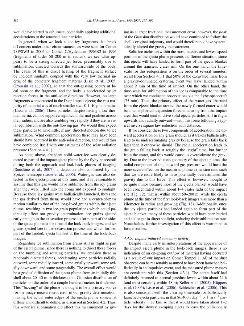
386 J.E. Richardson et al. / Icarus 190 (2007) 357–390
would have started to sublimate, potentially applying additionalaccelerations to the attached dust particles.
In general, when we look at the icy fragments that breakoff comets under other circumstances, as were seen for Comet73P/SW3 in 2006 or Comet C/Hyakutake 1996B2 in 1996(fragments of order 50–200 m in radius), we see what ap-pears to be a strong directed jet force, presumably due tosublimation, directed towards the sunward side of the body.The cause of this is direct heating of the fragment surfaceby incident sunlight, coupled with the very low thermal in-ertia of the cometary fragment material (Lisse et al., 2005;Groussin et al., 2007), so that the out-gassing occurs at lo-cal noon on the fragment, and the body is accelerated by jetreaction forces in the anti-solar direction. However, no largefragments were detected in the Deep Impact ejecta; the vast ma-jority of material was of much smaller size, 0.1–10 µm in radius(Lisse et al., 2006). These particles, despite having a low ther-mal inertia, cannot support a significant thermal gradient acrosstheir radius, and are also tumbling very rapidly if they are in vir-ial equilibrium with the out-flowing gas. We would thus expectthese particles to have little, if any, directed motion due to icesublimation. What common acceleration there may have beenshould have occurred in the anti-solar direction, and would thushave combined itself with our estimates of the solar radiationpressure (Section 4.4.1).
As noted above, abundant solid-water ice was clearly de-tected as part of the impact ejecta plume by the flyby-spacecraftduring both the approach and look-back phases of imaging(Sunshine et al., 2007), a detection also confirmed by theSpitzer telescope (Lisse et al., 2006). Water-gas was also de-tected in the ejecta plume at this time, and it is reasonable toassume that this gas would have sublimed from the icy grainsafter they were lifted into the coma and exposed to sunlight.Because these icy grains were ballistically launched, they (andthe gas derived from them) would have had a center-of-massmotion similar to that of the long-lived grains within the ejectaplume, resulting in two ice-grain populations which could po-tentially affect our gravity determination: ice grains ejectedearly enough in the excavation process to form part of the sidesof the ejecta plume at the time of the look-back images, and icegrains ejected late in the excavation process and which formedpart of the landed, ejecta blanket at the time of the look-backimages.
Regarding ice sublimation from grains still in flight as partof the ejecta plume, since there is nothing to direct these forceson the tumbling and rotating particles, we envision these asrandomly directed forces, accelerating some particles radiallyoutward, some radially inward, some axially upward, some axi-ally downward, and some tangentially. The overall effect wouldbe a gradual diffusion of the ejecta plume from an initially thinshell about 20–40 m in thickness to a Gaussian distribution ofparticles on the order of a couple hundred meters in thickness.This “fuzzing” of the plume is thought to be a primary sourcefor the image-measurement error in our gravity determination,making the actual outer edges of the ejecta plume somewhatdiffuse and difficult to define, as discussed in Section 4.2. Thus,this water ice sublimation did affect this measurement by giv-
ing us a larger fractional measurement error; however, the peakof the Gaussian distribution would have continued to follow theshell’s original trajectory, and would therefore not have system-atically altered the gravity measurement.
Solid ice inclusion within the most massive and lowest speedportions of the ejecta plume presents a different situation, sincethis ejecta will have landed to form part of the ejecta blanketaround the transient crater rim. On the one hand, the time-scale for this redeposition is on the order of several minutes:recall from Section 4.3.1 that 50% of the excavated mass froma gravity-dominated cratering event will have landed withinabout 9 min of the time of impact. On the other hand, thetime-scale for sublimation of this ice is comparable to the timeover which we conducted observations via the flyby-spacecraft(75 min). Thus, the primary effect of the water-gas liberatedfrom the ejecta blanket around the newly-formed crater wouldbe a hemispherical expansion force emanating from the impactarea that would tend to drive solid ejecta particles still in flightupwards and radially outward—with this force following a typ-ical inverse square law reduction with distance.
If we consider these two components of acceleration, the up-ward acceleration on any grain should, as it travels ballistically,lead to us underestimating gravity because the grain falls backlater than it otherwise should. The radial acceleration leads tothe grain falling back at roughly the “right” time, but furtherfrom the crater, and this would cause us overestimate the grav-ity. Due to the inverted-cone geometry of the ejecta plume, theradial component of this outward gas pressure would have themore severe effect on the measured plume expansion rate, suchthat we are more likely to have potentially overestimated thegravity due to this force. This effect is, however, thought tobe quite minor because most of the ejecta blanket would havebeen concentrated within about 1–4 crater radii of the impactsite (Fig. 12), that is, within about 50–200 m, while the ejectaplume at the time of the first look-back images was more than akilometer in radius and growing (Fig. 18). Additionally, oncethe icy ejecta particles had landed again to form part of theejecta blanket, many of these particles would have been buriedand no longer in direct sunlight, reducing their sublimation rate.Nonetheless, further investigation of this effect is warranted infuture studies.
4.4.5. Impact-induced cometary activityDespite many early misinterpretations of the appearance of
the impact ejecta plume in the look-back images, there is noindication of an on-going outflow of material having occurredas a result of our impact on Comet Tempel 1. All of the dustobserved can be reasonably assumed to have been launched bal-listically in an impulsive event, and the measured plume massesare consistent with this (Section 4.3.1). The comet itself haddefinitely returned to normal gas/dust levels within about 24 h(and most certainly within 48 h); Keller et al. (2005); Küpperset al. (2005); Lisse et al. (2006); Schleicher et al. (2006). Thisis also consistent with the clearing timescale for ballisticallylaunched ejecta particles, in that 86,400 s day−1 × 1 m s−1 par-ticle velocity = 87 km, so that it would have taken about 1–2days for the slowest escaping ejecta to leave the collisionally
Deep Impact ejecta plume analysis 387
Fig. 21. Deep Impact image sequence, part 1: a comparison between the actual HRI image sequence (upper images) and the best-fit modeled image sequence (lowerimages), using a Spitzer-based particle distribution (Lisse et al., 2006). The two pairs of images on the left show the early interior view of the ejecta plume (phase1), while the two pairs of images on the right show a near edge-on view of the plume’s west (upper left) side (phase 2).
thick zone of the coma and decouple fully from the nucleusoutflow. Also note that sublimation of water ice from the ejectablanket around the impact crater (Section 4.4.4) would appearto act like impact-induced activity from the crater itself, so carein identifying the correct source is necessary. Barring additionalevidence to the contrary, impact-induced cometary activity isnot considered to have had a significant effect on the observedejecta plume behavior.
5. Conclusion
In the process of this work, we felt it important to keepour model conservative with regard to the number of modelparameters, self-consistent throughout, and well grounded the-oretically: from the application of the π group scaling relation-ships for crater volume and formation time (Section 1.3), to theapplication of the Maxwell Z-model of excavation flow (Sec-tion 2.1), to the development of constants for the ejecta velocityscaling relationships (Section 2.2), to the addition of gravity andstrength affects to the model (Section 2.3), and finally to theempirically-based determination of ejecta launch angles (Sec-tions 2.4 and 2.5). Throughout its development, the number ofexperimentally determined constant values used by the modelhas been kept to a minimum, making use only of constantswhich are widely accepted and applicable to a wide range ofimpact environments (Table 2). At each point possible, we havechecked our model against previous work and the ejecta behav-ior recorded in recent experimental studies (Figs. 9–11).
Following model development, our stated goal in Section 1was to adjust the parameters of this model (over many iter-ations) to match the flyby-spacecraft observations of the ac-
tual plume behavior, image by image. Figs. 21 and 22 showeight examples from the final HRI image-sequence simulation,using the nominal model inputs from Table 2 and the deter-mined model parameters listed in Table 4. Also included is theSpitzer-based particle size distribution (PSD) from Lisse et al.(2006). The result is a synthetic image sequence which agreesquite well with the actual image sequence, despite the fact thatsecond-order effects, such as gaps and rays in the ejecta plume,have not been included: the ejecta plume goes smoothly throughall four viewing phases initially introduced in Fig. 1. While fur-ther refinements could be made, particularly in the area of ejectaplume opacity, the first-order match between actual and syn-thetic image sets is sufficient to meet the goals of this study.
This modeling exercise has indicated that Deep Impact pro-duced a reasonably “well-behaved” oblique-impact crateringevent: one in which the impactor–spacecraft apparently strucka small, westward-facing slope of roughly 1/3–1/2 the size ofthe final crater produced (determined from the initial ejectaplume geometry), and possessing an effective yield strengthof not more than Y = 1–10 kPa (estimated via two differentmethods). The resulting ejecta plume followed well-establishedscaling relationships for cratering in a medium-to-high poros-ity target material, consistent with a transient crater of notmore than 85–140 m diameter, formed in not more than 250–550 s, for the case of Y = 0 Pa (gravity-dominated cratering),and not less than 22–26 m diameter, formed in not less than1–3 s, for the case of Y = 10 kPa (strength-dominated crater-ing). At Y = 0 Pa, an upper limit to the total ejected mass of1.8 × 107 kg (1.5–2.2 × 10⁷ kg) is consistent with measure-ments made via long-range remote sensing, after taking intoaccount that 90% of this mass would have stayed close to the
388 J.E. Richardson et al. / Icarus 190 (2007) 357–390
Fig. 22. Deep Impact image sequence, part 2: a comparison between the actual HRI image sequence (upper images) and the best-fit modeled image sequence (lowerimages), using a Spitzer-based particle distribution (Lisse et al., 2006). The first pair of images on the left show the beginning of the transition from an edge-onview of the plume’s west side (phase 2) to the late interior view of the plume’s dark, oval base (phase 3): which is shown in the middle two pairs of images. Thesmall gray circle near the center of the middle two synthetic images marks the position of the impact crater, which the actual (upper) images failed to resolve due toobscuring dust. The final pair of images on the right show the beginning of the look-back phase of observations (phase 4).
surface and then landed within 45 min after the time of impact.However, at Y = 10 kPa, a lower limit to the total ejected massof 2.3 × 10⁵ kg (1.5–2.9 × 10⁵ kg) is also consistent with theremote sensing measurements—making this result somewhatambiguous. The expansion rate of the ejecta plume imagedduring the look-back phase of observations leads to an esti-mate of the comet’s mean surface gravity of g = 0.34 mm s−2
(0.17–0.90 mm s−2), which corresponds to a comet mass ofmt = 4.5 × 10¹³ kg (2.3–12.0 × 10¹³ kg) and a bulk density ofρt = 400 kg m−3 (200–1000 kg m−3), consistent with the bulkdensities estimated for other cometary nuclei, and where thehigh-end error is due to uncertainties in the magnitude of comagas pressure effects on the impact ejecta particles in flight (Sec-tion 4.4.2). These results are summarized in Table 4.
However, this work is a mathematical model of a physicalphenomena, and as such, it is important to keep in mind the as-sumptions that have gone into creating it: (1) the crater volumefollows the point-source assumption inherent in the π groupscaling relationships; (2) the π group scaling relationships canbe extended, reasonably well, into the realm of strength-dom-inated cratering in porous target materials for small impactswhich produce simple craters; (3) the cratering event followsthe Maxwell Z-model of excavation flow to first-order; and(4) the target material produces particle ejection angles whichare consistent with those produced by experimental impactsinto granular target materials, at both normal- and oblique-incidence. As with any such model, it is possible to find caseswhere the model breaks down: where its inherent assumptionshave been pushed too far. Of particular relevance to this work is
that our current understanding of the impact cratering processin highly porous targets, or targets possessing strength (particu-larly “weak” strength), is just at its beginning stages, and muchmore theoretical and experimental work needs to be done inthis area. In that respect, it was somewhat surprising to the au-thors that the cratering event produced by Deep Impact couldbe modeled as well as it can be—that the theory we have nowworks as well as it does. Nonetheless, there are still many as-pects of this event which are not understood, such as: what canwe learn from the prominent rays and gaps in the ejecta plume?How can the strength of the target at the impact site be con-strained further? Are there further temporal variations in theejecta plume which reflect additional spatial variations at theimpact site (such as layering)? What further role did volatilesplay in modifying the evolution of the impact ejecta plume?And, how can we better constrain the affects on the evolutionof the ejecta plume specifically due to the comet nucleus en-vironment? Even with a good first-order understanding of theDeep Impact event, which we believe we have reached withthis work, there is still much to be learned.
Acknowledgments
The authors would like to sincerely thank Keith Holsapple,Paul Weissman, and Mark Boslough for their patience and in-sightful reviews of this (large) work. They have helped to makethis a much better analysis and presentation than it was initially,and we have learned much in the process. We would also like

Deep Impact ejecta plume analysis 389
to thank Garrett Elliot for his assistance with the initial imageprocessing and data reduction necessary for this analysis.
References
A’Hearn, M.F., Belton, M.J.S., Delamere, A., Blume, W.H., 2005a. Deep Im-pact: A large-scale active experiment on a cometary nucleus. Space Sci.Rev. 117, 1–21.
A’Hearn, M.F., Belton, M.J.S., Delamere, W.A., Kissel, J., Klaasen, K.P., Mc-Fadden, L.A., Meech, K.J., Melosh, H.J., Schultz, P.H., Sunshine, J.M.,Thomas, P.C., Veverka, J., Yeomans, D.K., Baca, M.W., Busko, I., Crockett,C.J., Collins, S.M., Desnoyer, M., Eberhardy, C.A., Ernst, C.M., Farnham,T.L., Feaga, L., Groussin, O., Hampton, D., Ipatov, S.I., Li, J.-Y., Lindler,D., Lisse, C.M., Mastrodemos, N., Owen, W.M., Richardson, J.E., Well-nitz, D.D., White, R.L., 2005b. Deep Impact: Excavating Comet Tempel 1.Science 310, 258–264.
Anderson, J.L.B., Schultz, P.H., Heineck, J.T., 2003. Asymmetry of ejecta flowduring oblique impacts using three-dimensional particle image velocimetry.J. Geophys. Res. 108 (E8), doi:10.1029/2003JE002075.5094.
Anderson, J.L.B., Schultz, P.H., Heineck, J.T., 2004. Experimental ejectionangles for oblique impacts: Implications for the subsurface flow-field. Me-teorit. Planet. Sci. 39, 303–320.
Asphaug, E., Melosh, H.J., 1993. The Stickney impact of PHOBOS—A dy-namical model. Icarus 101, 144–164.
Austin, M.G., Thomsen, J.M., Ruhl, S.F., Orphal, D.L., Schultz, P.H., 1980.Calculational investigation of impact cratering dynamics: Material motionsduring the crater growth period. Lunar Planet. Sci. 11, 46–48.
Austin, M.G., Thomsen, J.M., Ruhl, S.F., Orphal, D.L., Borden, W.F., Lar-son, S.A., Schultz, P.H., 1981. Z-model analysis of impact cratering—Anoverview. In: Merill, R.B., Schultz, P.H. (Eds.), Multi-Ring Basins: Forma-tion and Evolution, Proceedings of the Lunar Planetary Science Conference,Houston, TX, November 10–12, 1980, Pergamon Press, New York, pp.197–205.
Bauer, J.M., Weissman, P.R., Choi, Y.-J., Troy, M., Young, J.W., Lisse, C.M.,Dekany, R., Hanner, M.S., Buratti, B.J., 2007. Palomar and Table Moun-tain observations of 9P/Tempel 1 during the Deep Impact encounter: Firstresults. Icarus 187, 296–305.
Buckingham, E., 1914. On physically similar systems; illustrations of the useof dimensional equations. Phys. Rev. 4 (4), 345–376.
Busko, I., Lindler, D., A’Hearn, M.F., White, R.L., 2007. Searching for theDeep Impact crater on Comet 9P/Tempel 1 using image processing tech-niques. Icarus 187, 56–68.
Chamberlain, J.W., Hunten, D.M., 1987. Theory of Planetary Atmospheres.Academic Press, San Diego.
Chapman, C.R., McKinnon, W.B., 1986. Cratering of planetary satellites. In:Burns, J.A., Matthews, M.S. (Eds.), Satellites, Univ. of Arizona Press, Tuc-son, pp. 492–580.
Cintala, M.J., Berthoud, L., Horz, F., 1999. Ejection-velocity distributions fromimpacts into coarse-grained sand. Meteorit. Planet. Sci. 34, 605–623.
Collins, G.S., Wünnemann, K., 2007. Numerical modeling of impact ejectionprocesses in porous targets. Lunar Planet. Sci. 38. 1789.
Croft, S.K., 1980. Cratering flow fields—Implications for the excavation andtransient expansion stages of crater formation. Lunar Planet. Sci. 11, 2347–2378.
Croft, S.K., 1981. The excavation stage of basin formation—A qualitativemodel. In: Merill, R.B., Schultz, P.H. (Eds.), Multi-Ring Basins: Forma-tion and Evolution, Proceedings of the Lunar Planetary Science Confer-ence, Houston, TX, November 10–12, 1980, Pergamon Press, New York,pp. 207–225.
Davidsson, B.J.R., Gutiérrez, P.J., 2004. Estimating the nucleus density ofComet 19P/Borrelly. Icarus 168, 392–408.
Davidsson, B.J.R., Gutiérrez, P.J., 2006. Non-gravitational force modeling ofComet 81P/Wild 2. Icarus 180, 224–242.
Davidsson, B.J.R., Gutiérrez, P.J., Rickman, H., 2007. Nucleus propertiesof Comet 9P/Tempel 1 estimated from non-gravitational force modeling.Icarus 187, 306–320.
Dienes, J.K., Walsh, J.M., 1970. Theory of impact: Some general principles andthe method of Eulerian codes. In: Kinslov, K. (Ed.), High-Velocity ImpactPhenomena. Academic Press, New York, pp. 1–579.
Durda, D.D., 2004. Ejecta generation and redistribution on 433 Eros: Modelingejecta launch conditions. Lunar Planet. Sci. 35. 1096.
Elbeshausen, D., Wünnemann, K., Collins, G.S., 2007. Three-dimensional nu-merical modeling of oblique impact processes: Scaling of cratering effi-ciency. Lunar Planet. Sci. 38. 1952.
Farnham, T.L., Cochran, A.L., 2002. A McDonald Observatory study of Comet19P/Borrelly: Placing the Deep Space 1 observations into a broader context.Icarus 160, 398–418.
Fernández, Y.R., Lisse, C.M., Kelley, M.S., Dello Russo, N., Tokunaga, A.T.,Woodward, C.E., Wooden, D.H., 2007. Near-infrared light curve of Comet9P/Tempel 1 during Deep Impact. Icarus 187, 220–227.
Finson, M.L., Probstein, R.F., 1968. A theory of dust comets. I. Model andequations. Astrophys. J. 154, 353–380.
Gault, D.E., Wedekind, J.A., 1978. Experimental studies of oblique impact.Lunar Planet. Sci. 9, 374–376.
Geissler, P., Petit, J., Durda, D.D., Greenberg, R., Bottke, W., Nolan, M.,Moore, J., 1996. Erosion and ejecta reaccretion on 243 Ida and its moon.Icarus 120, 140–157.
Grady, D.E., Kipp, M.E., 1987. Dynamic rock fragmentation. In: Atkinson,B.K. (Ed.), Fracture Mechanics of Rock. Academic Press, London, pp. 429–475.
Groussin, O., A’Hearn, M.F., Li, J.-Y., Thomas, P.C., Sunshine, J.M., Lisse,C.M., Meech, K.J., Farnham, T.L., Feaga, L.M., Delamere, W.A., 2007.Surface temperature of the nucleus of Comet 9P/Tempel 1. Icarus 187, 16–25.
Hampton, D.L., Baer, J.W., Huisjen, M.A., Varner, C.C., Delamere, A., Well-nitz, D.D., A’Hearn, M.F., Klaasen, K.P., 2005. An overview of the instru-ment suite for the Deep Impact mission. Space Sci. Rev. 117, 43–93.
Harker, D.E., Woodward, C.E., Wooden, D.H., 2005. The dust grains from9P/Tempel 1 before and after the encounter with Deep Impact. Science 310,278–280.
Holsapple, K.A., 1993. The scaling of impact processes in planetary sciences.Annu. Rev. Earth Planet. Sci. 21, 333–373.
Holsapple, K.A., Housen, K.R., 2007. A crater and its ejecta: An interpretationof Deep Impact. Icarus 187, 345–356.
Holsapple, K.A., Schmidt, R.M., 1980. On the scaling of crater dimensions.I. Explosive processes. J. Geophys. Res. 85, 7247–7256.
Holsapple, K.A., Schmidt, R.M., 1982. On the scaling of crater dimensions.II. Impact processes. J. Geophys. Res. 87, 1849–1870.
Holsapple, K.A., Schmidt, R.M., 1987. Point source solutions and couplingparameters in cratering mechanics. J. Geophys. Res. 92, 6350–6376.
Housen, K.R., Holsapple, K.A., 2003. Impact cratering on porous asteroids.Icarus 163, 102–119.
Housen, K.R., Schmidt, R.M., Holsapple, K.A., 1983. Crater ejecta scalinglaws—Fundamental forms based on dimensional analysis. J. Geophys.Res 88 (17), 2485–2499.
Keller, H.U., Jorda, L., Küppers, M., Gutierrez, P.J., Hviid, S.F., Knollenberg,J., Lara, L.-M., Sierks, H., Barbieri, C., Lamy, P., Rickman, H., Rodrigo, R.,2005. Deep Impact observations by OSIRIS onboard the Rosetta spacecraft.Science 310, 281–283.
Keller, H.U., Küppers, M., Fornasier, S., Gutiérrez, P.J., Hviid, S.F., Jorda, L.,Knollenberg, J., Lowry, S.C., Rengel, M., Bertini, I., Cremonese, G., Ip, W.-H., Koschny, D., Kramm, R., Kührt, E., Lara, L.-M., Sierks, H., Thomas,N., Barbieri, C., Lamy, P., Rickman, H., Rodrigo, R., A’Hearn, M.F., An-grilli, F., Barucci, M.-A., Bertaux, J.-L., da Deppo, V., Davidsson, B.J.R.,de Cecco, M., Debei, S., Fulle, M., Gliem, F., Groussin, O., Lopez Moreno,J.J., Marzari, F., Naletto, G., Sabau, L., Sanz Andrés, A., Wenzel, K.-P.,2007. Observations of Comet 9P/Tempel 1 around the Deep Impact eventby the OSIRIS cameras onboard Rosetta. Icarus 187, 87–103.
Knight, M.M., Walsh, K.J., A’Hearn, M.F., Swaters, R.A., Zauderer, B.A.,Samarasinha, N.H., Vázquez, R., Reitsema, H., 2007. Ground-based visi-ble and near-IR observations of Comet 9P/Tempel 1 during the Deep Impactencounter. Icarus 187, 199–207.
Küppers, M., Bertini, I., Fornasier, S., Gutierrez, P.J., Hviid, S.F., Jorda, L.,Keller, H.U., Knollenberg, J., Koschny, D., Kramm, R., Lara, L.-M., Sierks,
390 J.E. Richardson et al. / Icarus 190 (2007) 357–390
H., Thomas, N., Barbieri, C., Lamy, P., Rickman, H., Rodrigo, R., A’Hearn,M.F., Angrilli, F., Bailey, M.E., Barthol, P., Barucci, M.A., Bertaux, J.-L.,Burns, J.A., Cremonese, G., Curdt, W., De Cecco, M., Debei, S., Fulle, M.,Gliem, F., Ip, W.-H., Kührt, E., Llebaria, A., Lopez Moreno, J.J., Marzari,F., Naletto, G., Sabau, L., Sanz Andrés, A., Sivan, J.P., Tondello, G., Wen-zel, K.-P., 2005. A large dust/ice ratio in the nucleus of Comet 9P/Tempel 1.Nature 437, 987–990.
Lamy, P.L., Toth, I., Davidsson, B.J.R., Groussin, O., Gutiérrez, P., Jorda, L.,Kaasalainen, M., Lowry, S.C., 2007. A portrait of the nucleus of Comet67P/Churyumov–Gerasimenko. Space Sci. Rev. 128, 23–66.
Larson, E.E., 1977. The Relationship of Rock Properties to Explosive En-ergy Coupling, UCRL-52204. University of California Research Labs, NewYork.
Lisse, C.M., A’Hearn, M.F., Hauser, M.G., Kelsall, T., Lien, D.J., Moseley,S.H., Reach, W.T., Silverberg, R.F., 1998. Infrared observations of cometsby COBE. Astrophys. J. 496, 971–991.
Lisse, C.M., A’Hearn, M.F., Groussin, O., Fernández, Y.R., Belton, M.J.S.,van Cleve, J.E., Charmandaris, V., Meech, K.J., McGleam, C., 2005. Ro-tationally resolved 8–35 micron Spitzer Space Telescope observations ofthe nucleus of Comet 9P/Tempel 1. Astrophys. J. 625, L139–L142.
Lisse, C.M., VanCleve, J., Adams, A.C., A’Hearn, M.F., Fernández, Y.R., Farn-ham, T.L., Armus, L., Grillmair, C.J., Ingalls, J., Belton, M.J.S., Groussin,O., McFadden, L.A., Meech, K.J., Schultz, P.H., Clark, B.C., Feaga, L.M.,Sunshine, J.M., 2006. Spitzer spectral observations of the Deep Impactejecta. Science 313, 635–640.
Mason, K.O., Chester, M., Cucchiara, A., Gronwall, C., Grupe, D., Hunsberger,S., Jones, G.H., Koch, S., Nousek, J., O’Brien, P.T., Racusin, J., Roming,P., Smith, P., Wells, A., Willingale, R., Branduardi-Raymont, G., Gehrels,N., 2007. Swift ultraviolet photometry of the Deep Impact encounter withComet 9P/Tempel 1. Icarus 187, 123–131.
Maxwell, D., Seifert, K., 1974. Modeling of cratering, close-in displacements,and ejecta. Report DNA 3628F, Defense Nuclear Agency, Washington, DC.
Maxwell, D.E., 1977. Simple Z model of cratering, ejection, and overturnedflap. In: Roddy, D,J., Pepin, R.O., Merrill, R.B. (Eds.), Impact and Explo-sion Cratering. Pergamon, Elmsford, NY, pp. 1003–1008.
McEwen, A.S., 1991. Photometric functions for photoclinometry and other ap-plications. Icarus 92, 298–311.
Melosh, H.J., 1989. Impact Cratering: A Geologic Process. Oxford Univ. Press,New York.
Melosh, H.J., 2001. Gravitational modification of ejecta curtain expansion. Lu-nar Planet. Sci. 32, 2135.
Melosh, H.J., Ryan, E.V., Asphaug, E., 1992. Dynamic fragmentation inimpacts—Hydrocode simulation of laboratory impacts. J. Geophys. Res.97, 14735–14759.
Melosh, H.J., A’Hearn, M.F., Belton, M.J.S., Delamere, W.A., Kissel, J.,Klaasen, K.P., McFadden, L.A., Meech, K.J., Schultz, P.H., Sunshine, J.M.,Thomas, P.C., Veverka, J., Yeomans, D.K., Baca, M.W., Busko, I., Crockett,C.J., Collins, S.M., Desnoyer, M., Eberhardy, C.A., Ernst, C.M., Farnham,T.L., Feaga, L., Groussin, O., Hampton, D., Ipatov, S.I., Li, J.-Y., Lindler,D., Lisse, C.M., Mastrodemos, N., Owen, W.M., Richardson, J.E., Well-nitz, D.D., White, R.L., 2006. Deep Impact: The first second. Lunar Planet.Sci. 37, 1165.
Milani, G.A., Szabó, G.M., Sostero, G., Trabatti, R., Ligustri, R., Nicolini, M.,Facchini, M., Tirelli, D., Carosati, D., Vinante, C., Higgins, D., 2007. Pho-tometry of Comet 9P/Tempel 1 during the 2004/2005 approach and theDeep Impact module impact. Icarus 187, 276–284.
Nolan, M.C., Asphaug, E., Melosh, H.J., Greenberg, R., 1996. Impact craters onasteroids: Does gravity or strength control their size? Icarus 124, 359–371.
Pierazzo, E., Melosh, H.J., 2000. Understanding oblique impacts from experi-ments, observations, and modeling. Annu. Rev. Earth Planet. Sci. 28, 141–167.
Press, W.H., Teukolsky, S.A., Vetterling, W.T., Flannery, B.P., 1992. NumericalRecipes in FORTRAN 77. Cambridge Univ. Press, Cambridge.
Richardson, J.E., Melosh, H.J., Artemeiva, N.A., Pierazzo, E., 2005. Impactcratering theory and modeling for the Deep Impact mission: From missionplanning to data analysis. Space Sci. Rev. 117, 241–267.
Schleicher, D.G., Barnes, K.L., Baugh, N.F., 2006. Photometry and imagingresults for Comet 9P/Tempel 1 and Deep Impact: Gas production rates,postimpact light curves, and ejecta plume morphology. Astron. J. 131,1130–1137.
Schmidt, R.M., Housen, K.R., 1987. Some recent advances in the scaling ofimpact and explosion cratering. Int. J. Impact Eng. 5, 543–560.
Schultz, P.H., Ernst, C.M., Anderson, J.L.B., 2005. Expectations for cratersize and photometric evolution from the Deep Impact collision. Space Sci.Rev. 117, 207–239.
Schultz, P.H., Eberhardy, C.A., Ernst, C.M., A’Hearn, M.F., Sunshine, J.M.,Lisse, C.M., 2007. The Deep Impact oblique impact cratering experiment.Icarus 190, 295–333.
Sugita, S., Ootsubo, T., Kadono, T., Honda, M., Sako, S., Miyata, T., Sakon, I.,Yamashita, T., Kawakita, H., Fujiwara, H., Fujiyoshi, T., Takato, N., Fuse,T., Watanabe, J., Furusho, R., Hasegawa, S., Kasuga, T., Sekiguchi, T., Ki-noshita, D., Meech, K.J., Wooden, D.H., Ip, W.H., A’Hearn, M.F., 2005.Subaru Telescope observations of Deep Impact. Science 310, 274–278.
Sunshine, J.M., Groussin, O., Schultz, P.H., A’Hearn, M.F., Feaga, L.M., Farn-ham, T.L., Klassen, K.P., 2007. The distribution of water ice in the interiorof Comet Tempel 1. Icarus 190, 284–294.
Thomas, P.C., Veverka, J., A’Hearn, M.F., McFadden, L., Belton, M.J.S., Sun-shine, J.M., 2005. Comet geology with Deep Impact remote sensing. SpaceSci. Rev. 117, 193–205.
Thomas, P.C., Veverka, J., Belton, M.J.S., Hidy, A., A’Hearn, M.F., Farnham,T.L., Groussin, O., Li, J.-Y., McFadden, L.A., Sunshine, J., Wellnitz, D.,Lisse, C., Schultz, P., Meech, K.J., Delamere, W.A., 2007. The shape,topography, and geology of Tempel 1 from Deep Impact observations.Icarus 187, 4–15.
Thomsen, J.M., Austin, M.G., Ruhl, S.F., Orphal, D.L., Schultz, P.H., 1980a.The detailed application of Maxwell’s Z-model to laboratory-scale impactcratering calculations. LPI Contribution 414, p. 92.
Thomsen, J.M., Austin, M.G., Schultz, P.H., 1980b. The development of theejecta plume in a Laboratory-Scale Impact Cratering Event. Lunar Planet.Sci. 11, 1146–1148.
Turcotte, D.L., Schubert, G., 2002. Geodynamics. In: Turcotte, D.L., Schu-bert, G. (Eds.), Geodynamics. Cambridge Univ. Press, Cambridge, UK,ISBN 0521661862, p. 472.
Weissman, P.R., Asphaug, E., Lowry, S.C., 2004. Structure and densityof cometary nuclei. In: Feston, M.C., Keller, H.U., Weaver, A. (Eds.),Comets II. Univ. of Arizona Press, Tucson, pp. 337–357.
Werner, R.A., 1994. The gravitational potential of a homogeneous polyhedronor don’t cut corners. Celest. Mech. Dynam. Astron. 59, 253–278.
Wünnemann, K., Collins, G.S., Melosh, H.J., 2006. A strain-based porositymodel for use in hydrocode simulations of impacts and implications fortransient crater growth in porous targets. Icarus 180, 514–527.