Verification and Presburger Arithmetic

A. Ada & K. Sutner

Carnegie Mellon University

Spring 2018

1 Prelude

Presburger Arithmetic

Synchronous Relations

Deciding Presburger Arithmetic

Pentium FDIV Bug 3

Floating Point Error 4

4195835.0/3145727.0 = 1.3338204491362410025 correct

4195835.0/3145727.0 = 1.3337390689020375894 pentium

Alternatively

4195835.0− 3145727.0 ∗ (4195835.0/3145727.0) = 0 correct

4195835.0− 3145727.0 ∗ (4195835.0/3145727.0) = 256 pentium

This fatal bug was discovered in October 1994 by number theorist Thomas R.Nicely, doing research in pure math. Intel did not respond well, and lost around$ 500 mill.

Incidentally, this is a software problem at heart.

Turing Award 2007 5

If applied, Clarke’s model checking methods would have found the bug.

More importantly, they were powerful enough to prove that the patch Intelconcocted was indeed correct.

Ariane V 6

The Disaster 7

On June 4, 1996, the maiden flight of the European Ariane 5 rocket crashedabout 40 seconds after takeoff. The direct financial loss was about half abillion dollars, all uninsured. An investigation showed that the explosion wasthe result of a software error.

Particularly annoying is the fact that the problem came from a piece of thesoftware that was not needed during the crash, the Inertial Reference System.Before lift-off certain computations are performed to align the IRS. Normallythey should be stopped at −9 seconds. However, a hold in the countdownwould require a reset of the IRS taking several hours.

The Cause 8

To avoid this nuisance, the computation was allowed to continue even after thesystem had switched to flight mode.

In the Ariane 5, this caused an uncaught exception due to a floating-pointerror: a conversion from a 64-bit integer (which should have been less than215) to a 16-bit signed integer was erroneously applied to a greater number:the “horizontal bias” of the flight depends much on the size of rocket–andAriane 5 was larger than its predecessors.

There was no explicit exception handler (since it presumably was not needed),so the entire software crashed and the launcher with it.

Logic is Hard 9

Everybody who has worked in formal logic will confirm that it is one ofthe technically most refractory parts of mathematics. The reason forthis is that it deals with rigid, all-or-none concepts, and has very littlecontact with the continuous concept of the real or of the complex num-ber, that is, with mathematical analysis. Yet analysis is the technicallymost successful and best-elaborated part of mathematics. Thus formallogic is, by the nature of its approach, cut off from the best cultivatedportions of mathematics, and forced onto the most difficult part of themathematical terrain, into combinatorics.

John von Neumann, 1948

Software is Applied Logic 10

There are lots of proposals floating around the problem of constructing correctsoftware. None of them gets around the fundamental problem:

Software is applied logic.

And, logic is hard, even for a super-genius like von Neumann.

The Good News: Logic also provides very powerful tools that help in theconstruction of correct code.

Prelude

2 Presburger Arithmetic

Synchronous Relations

Deciding Presburger Arithmetic

A Verification Problem 12

Suppose you are implementing a dynamic programming algorithm that has tofill out an n× n array A. The algorithm

initializes the first row and the first column,

then fills in the whole array according to

A[i, j] = func(A[i− 1, j], A[i, j − 1])

lastly, reads off the result in A[n− 1, n− 1].

We would like to check that all the array access operations are safe, and thatthe result is properly computed.

And, we want to do so automatically.

Filling In 13

One of the problems is that the recurrence can be implemented in several ways:

// column by column

for i = 1 .. n-1 do

for j = 1 .. n-1 do

A[i,j] = func( A[i-1,j], A[i,j-1] )

// row by row

for j = 1 .. n-1 do

for i = 1 .. n-1 do

A[i,j] = func( A[i-1,j], A[i,j-1] )

// by diagonal

for d = 1 .. 2n-3 do

for i = 1 .. d do

A[i,d-i+1] = func( A[i-1,d-i+1], A[i,d-i] )

Correctness 14

For a human, it is easy to see that the row-by-row and column-by-columnmethods are correct.

The diagonal approach already requires a bit of thought: why 2n− 3?

The good news is that the index arithmetic involved in the algorithms is quitesimple, essentially all we need is addition and order.

That is very fortunate, since arithmetic in general is a tough nut to crack.

Recall: Matiyasevic 15

Theorem (Y. Matiyasevic, 1970)

It is undecidable whether a Diophantine equation has a solution in the integers.

Suppose we wanted to build a reasoning system for ordinary Peano Arithmetic(PA). So we are trying to axiomatize the structure

N = 〈N,+, ∗, 0, 1;< 〉

Peano figured out how to do this in 1889; similar arrangements work for Z.

But there is a problem: the terms in (PA) are essentially polynomials withintegral coefficients:

t(x) =∑ece xe

where xe = xe11 xe22 . . . x

ekk .

Existential Theory 16

Matiyasevic’s theorem implies that it is undecidable whether a formula

∃x (t(x) = 0)

is true. Never mind more complicated formulae with alternating quantifiers andthe like:

∀x (even(x) ∧ x ≥ 4 ⇒ ∃u, v (x = u+ v ∧ prime(u) ∧ prime(v))

If we want to reason about arithmetic, we need to use something weaker thanPeano arithmetic.

Here is a radical proposal: let’s just forget about multiplication.

Presburger Arithmetic 17

We restrict ourselves to the structure

N− = 〈N,+, 0, 1;< 〉

The terms in this language are pretty weak:

t(x) = c+∑

cixi

where all the c, ci are constant. This is easy to check by induction.

In particular, we have lost multivariate polynomials–which is a good thing.

Semilinear Sets 18

Definition

A set A ⊆ N is linear if A = c+∑cixi | xi ≥ 0 .

A set A ⊆ N is semilinear if it is the finite union of linear sets.

Clearly, semilinear sets are definable in Presburger Arithmetic:

z ∈ A ⇐⇒ ∃x(t1(x) = z ∨ t2(x) = z ∨ . . . ∨ tk(x) = z

)

Theorem

The sets definable in Presburger Arithmetic are exactly the semilinear sets.

This is rather surprising: your intuition might tell you that more complicatedquantifier structures would produce more complicated sets.

Digression: Tally Languages 19

Suppose we code natural numbers in unary: n 7→ an.

Then every set A ⊆ N corresponds to a tally language A′ ⊆ a?.

Theorem

A set A ⊆ N is semilinear if, and only if, A′ is regular.

Exercise

Prove the theorem: figure out what all DFAs over a one-letter alphabet looklike.

Presburger’s Approach 20

Presburger used an important method called quantifier elimination: bytransforming a formula into another, equivalent one that has one fewerquantifiers. Ultimately, we can get rid of all quantifiers.

The remaining quantifier-free formula is equivalent to the original one, and iseasily tested for validity.

So a single step takes us from

Φ = ∃x1 ∀x2 ∃x3 . . .∃ z ϕ(z,x)

to an equivalent formula

Φ ≡ Φ′ = ∃x1 ∀x2 ∃x3 . . . ϕ′(x)

where the elimination variable z is no longer present.

Universal quantifiers are handled via ∀ ≡ ¬∃¬.

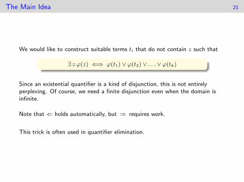
The Main Idea 21

We would like to construct suitable terms ti that do not contain z such that

∃ z ϕ(z) ⇐⇒ ϕ(t1) ∨ ϕ(t2) ∨ . . . ∨ ϕ(tk)

Since an existential quantifier is a kind of disjunction, this is not entirelyperplexing. Of course, we need a finite disjunction even when the domain isinfinite.

Note that ⇐ holds automatically, but ⇒ requires work.

This trick is often used in quantifier elimination.

Boosting the Language 22

To construct these terms we first have to augment our language a bit (QE failsfor the smaller language).

Add the subtraction operation x− y.

Add a constant c for each integer.

Add a multiplication function λx.c ∗ x for each integer c.

Add a divisibility predicate c | x for each integer c.

These additions do not change the expressiveness of our system, they just makeit easier to write things down: 3 ∗ x instead of x+ x+ x, 3 | x instead of∃ z (z + z + z = x).

Note that all terms are still linear despite the additions to the language.

Using Normal Forms 23

We may safely assume that ϕ is in disjunctive normal form. Since

∃ z (ϕ1(z) ∨ ϕ2(z)) ⇐⇒ ∃ z (ϕ1(z)) ∨ ∃ z (ϕ2(z))

it suffices to remove a quantifier from a conjunction of atomic formulae, say

ϕ = ϕ1 ∧ ϕ2 ∧ . . . ∧ ϕk

where the ϕi are quantifier-free.

The ϕi will contain z and possibly other free variables (which are bound in thebig formula by other quantifiers).

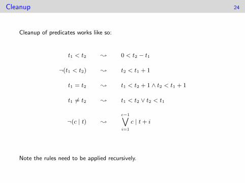
Cleanup 24

Cleanup of predicates works like so:

t1 < t2 ; 0 < t2 − t1

¬(t1 < t2) ; t2 < t1 + 1

t1 = t2 ; t1 < t2 + 1 ∧ t2 < t1 + 1

t1 6= t2 ; t1 < t2 ∨ t2 < t1

¬(c | t) ;

c−1∨i=1

c | t+ i

Note the rules need to be applied recursively.

Now What? 25

We are left with a conjunction that consists of atomic pieces

0 < t c | t

with linear terms t that may contain the elimination variable z.

Observation:

0 < t ⇐⇒ 0 < kt c | t ⇐⇒ kc | kt

for any positive k.

So we can manipulate the coefficients next to z in all terms containing z.

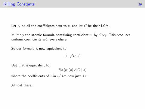
Killing Constants 26

Let ci be all the coefficients next to z, and let C be their LCM.

Multiply the atomic formula containing coefficient ci by C/ci. This producesuniform coefficients ±C everywhere.

So our formula is now equivalent to

∃ z ϕ′(Cz)

But that is equivalent to∃ z (ϕ′(z) ∧ C | z)

where the coefficients of z in ϕ′ are now just ±1.

Almost there.

The Vanishing Variable 27

We can rearrange things a bit to get a formula that looks like

ψ(z) =∧ai < z ∧

∧z < bj ∧

∧dk | z + tk

First, for simplicity, let’s ignore the divisibility constraints. Then the lastformula is clearly equivalent to max ai + 1 < min bj which is equivalent to∧

ij

ai + 1 < bj

Et voila: the pesky z is gone.

Test Terms 28

This can can also be expressed using test terms:

α∨i=1

ψ(ai + 1)

And we can handle divisibility constraints

α∨i=1

D∨j=1

ψ(ai + j)

where D is the LCM of all the di.

The case when there are no lower bounds on z is similar.

Presburger Arithmetic is Decidable 29

It follows that first-order logic for arithmetic without multiplication isdecidable.

It should be clear from the quantifier elimination process given here that animplementation is somewhat messy.

Worse, it turns out that the computational complexity of Presburger arithmeticis pretty bad:

Ω(22cn) and O(222cn

)

Prelude

Presburger Arithmetic

3 Synchronous Relations

Deciding Presburger Arithmetic

Getting Rid of Proof Theory 31

The last argument is really an exercise in proof theory: we have shown that acertain theory (augmented Presburger) can establish equivalences

∃ z ϕ(z) ⇐⇒ ϕ′

This is great, but perhaps there is an alternative approach that does notdepend quite so heavily on syntactic details?

An approach grounded in semantics rather than proofs?

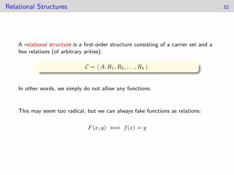
Relational Structures 32

A relational structure is a first-order structure consisting of a carrier set and afew relations (of arbitrary arities):

C = 〈A;R1, R2, . . . , Rk 〉

In other words, we simply do not allow any functions.

This may seem too radical, but we can always fake functions as relations:

F (x, y) ⇐⇒ f(x) = y

White Lie 33

All true, but note that a purely relational vocubulary makes our formulae a bitmore complicated.

For example, consider the formula

f(f(x)) = y

There really is a hidden quantifier:

∃ z (f(x) = z ∧ f(z) = y)

and so any decision algorithm has to cope with this invisible quantifier.

In a purely relational structure everything is out in the open, we have to writesomething like

∃ z (F (x, z) ∧ F (z, y))

FSMs to the Rescue 34

So the structures we are interested in have the restricted form

C = 〈A;R1, R2, . . . 〉

where

A ⊆ Σ? is a regular set of words, and

Ri ⊆ Aki , a rational relation.

Note that this trivially includes all finite structures.

But we also can easily express infinite sets like N or Z in this manner.

Bummer 35

The question is whether rational relations

are expressive enough to write down interesting properties,

are well-behaved enough for us to decide whether a first-order formulaholds over such a structure.

The answer to question 1 is mostly yes.

But question 2 gets a loud NO: we already know that rational relations are notclosed under intersection and complement.

Scaling Back 36

Rational relations in general are just a little too powerful for our purposes, weneed to scale back a bit.

One sledge-hammer restriction is to insist that all the relations arelength-preserving. In this case we have, say, R ⊆ (Σ× Γ)?, so we are actuallydealing with words over the product alphabet Σ× Γ.

These can be checked by an ordinary one-tape FSM over this product alphabet:

x1 x2 . . . xny1 y2 . . . yn

Relaxing the Length Condition 37

Alas, length-preserving relations are bit too restricted for our purposes. To dealwith words of different lengths, first extend each component alphabet by apadding symbol #: Σ# = Σ ∪ # where # /∈ Σ.

The alphabet for “two-track” words is ∆# = Σ# × Γ#.

This pair of padded words is called the convolution of x and y and is oftenwritten x:y.

x:y =x1 x2 . . . xn # . . . #

y1 y2 . . . yn yn+1 . . . ym

Another example of bad terminology, convolutions usually involve differentdirections.

Two Comments 38

Note that we are not using all of ∆?# but only the regular subset coming from

convolutions. For example,

a # b #

a b a #

is not allowed.

As always, a similar approach clearly works for kary relations

Σ1,# × Σ2,# × . . .× Σk,#

Exercise

Show that the collection of all convolutions forms a regular language.

Synchronous Relations 39

Here is an idea going back to Buchi and Elgot in 1965.

Definition

A relation ρ ⊆ Σ? × Γ? is synchronous or automatic if there is a finite statemachine A over ∆# such that

L(A) = x:y | ρ(x, y) ⊆ ∆?#

k-ary relations are treated similarly.

Note that this machine A is just a language recognizer, not a transducer: sincewe pad, we can read one symbol in each track at each step. We can alwayschoose A to be a DFA (though efficiency may be better with nondeterministicmachines).

Again . . . 40

In a sense, synchronous relations are the most basic examples of relations thatare not entirely trivial: given two words x and y, we pad out the shorter wordto get equal length

x1 x2 . . . xn # . . . #

y1 y2 . . . yn yn+1 . . . ym

and then a one-tape DFA reads two symbols (xi, yi) or (#, yi) at each step.

By contrast, one sometimes refers to arbitrary rational relations asasynchronous: we need two tapes and the two heads can separate arbitrarily far.

(Counter)Examples 41

Lexicographic order is synchronous.

The prefix-relation is synchronous.

The ternary addition relation is synchronous.

The suffix-relation is not synchronous.

The relations “x is a factor of y” and “x is a subword of y” are notsynchronous.

A Justification 42

Our motivation for synchronous relations was taken from length-preservingrelations. The reason this works out in the end is the following surprisingresult.

Theorem (Elgot, Mezei 1965)

Any length-preserving rational relation is already synchronous.

Note that this sounds utterly fishy: why should we be able to synchronize thetwo heads to move in lockstep? All we know is that in the end they will havetaken the same number of steps.

The proof is quite messy, we’ll skip.

Boolean Operations 43

Claim

Synchronous relations are closed under union, intersection and complement.

The proof is very similar to the argument for regular languages: one caneffectively construct the corresponding automata using the standard productmachine idea.

This is a hugely important difference between general rational relations andsynchronous relations: the latter do form an effective Boolean algebra, but wehave already seen that the former are not closed under intersection (norcomplement).

Warning: Concatenation 44

Synchronous relations are not closed under concatenation (or Kleene star). Forexample, let

R =(aε

)?( εa

)?S =

(bb

)?Then both R and S are synchronous, but R · S is not (the dot here isconcatenation, not composition).

Exercise

Prove all examples and counterexamples.

Synchronous Composition 45

On the upside, synchronous relations are closed under composition.

Suppose we have two binary relations R ⊆ Σ? × Γ? and S ⊆ Γ? ×∆?.

Theorem

If both R and S are synchronous relations, then so is their composition R S.

Exercise

Prove the theorem.

Synchronous Projections 46

More good news: synchronous relations are closed under projections.

Lemma

Whenever R is synchronous, so is its projection R′.

The argument is verbatim the same as for general rational relations: we erase atrack in the labels.

Again, this will generally produce a nondeterministic transition system even ifwe start from a deterministic one. If we also need complementation to dealwith logical negation we may have to deal with exponential blow-up.

Prelude

Presburger Arithmetic

Synchronous Relations

4 Deciding Presburger Arithmetic

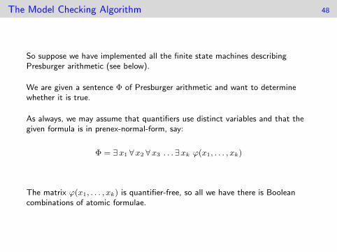
The Model Checking Algorithm 48

So suppose we have implemented all the finite state machines describingPresburger arithmetic (see below).

We are given a sentence Φ of Presburger arithmetic and want to determinewhether it is true.

As always, we may assume that quantifiers use distinct variables and that thegiven formula is in prenex-normal-form, say:

Φ = ∃x1 ∀x2 ∀x3 . . .∃xk ϕ(x1, . . . , xk)

The matrix ϕ(x1, . . . , xk) is quantifier-free, so all we have there is Booleancombinations of atomic formulae.

Atomic 49

In our case, there are only three possible atomic cases:

x = y

x < y

x+ y = z

Given actual strings for the variables, these can be tested by synchronoustransducers A=, A< and A+ (2, 2, and 3 tracks, respectively).

Strictly speaking, we can also say x = 0 and x = 1, but that is straightforwardto deal with.

From Atomic to Quantifier-Free 50

Back to the matrix, the quantifier-free formula

ϕ(x1, x2, . . . , xk)

with all variables as shown. We construct a k-track machine by induction onthe subformulae of ϕ.

The atomic pieces read from the appropriate tracks and check thecorresponding relation using the given transducers.

More precisely, we use variants such as A=,x,y to check that the strings in thex and y track are equal.

These machines can all be defined over the joint alphabet 0, 1,#k (thougheach machine only needs a few of the bits). Note that the alphabet growsexponentially with k, so there is an efficiency problem.

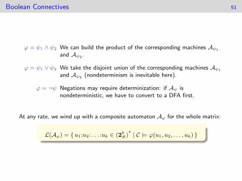
Boolean Connectives 51

ϕ = ψ1 ∧ ψ2 We can build the product of the corresponding machines Aψ1

and Aψ2 .

ϕ = ψ1 ∨ ψ2 We take the disjoint union of the corresponding machines Aψ1

and Aψ2 (nondeterminism is inevitable here).

ϕ = ¬ψ Negations may require determinization: if Aψ isnondeterministic, we have to convert to a DFA first.

At any rate, we wind up with a composite automaton Aϕ for the whole matrix:

L(Aϕ) = u1:u2: . . . :uk ∈ (2k#)? | C |= ϕ(u1, u2, . . . , uk)

Quantifiers 52

It remains to deal with quantifiers. We will work on the innermost quantifier,say

∃ z ϕ(z)

We have a machine Aϕ that has a track for variable z.

Simply erase the z-track from all the transition labels.

This corresponds exactly to existential quantification, done!

For universal quantifiers we use the old equivalence ∀ ≡ ¬∃ ¬.

This is all permissible, since projections and negations do not disturbautomaticity.

Finale Furioso 53

In the process of removing quantifiers, we lose one track at each step (butremember that universal quantifiers cause quite a bit additional activity).

In the end, we wind up with an unlabeled transition system: just a directedgraph, all edge-labels are gone. This transition system has a path from I to Fiff the original sentence Φ is valid.

So the final test is nearly trivial: plain DFS works fine.

Alas, it does take a bit of work to construct this digraph in the first place.

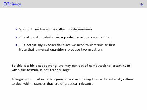
Efficiency 54

∨ and ∃ are linear if we allow nondeterminism.

∧ is at most quadratic via a product machine construction.

¬ is potentially exponential since we need to determinize first.Note that universal quantifiers produce two negations.

So this is a bit disappointing: we may run out of computational steam evenwhen the formula is not terribly large.

A huge amount of work has gone into streamlining this and similar algorithmsto deal with instances that are of practical relevance.

Implementing N− 55

There are several choices for the representation of natural numbers:

binary (MSD first)

binary (MSD first), no leading 0’s

reverse binary (LSD first)

reverse binary (LSD first), no trailing 0’s

ε denotes/does not denote 0

They all work equally well, but note that the machines implementing therelations will be slightly different.

Let’s assume options 4 and no ε.

Relations 56

addition as a ternary relation α

“constants” zero and one as unary relations

order less as a binary relation

These are all synchronous, regardless of how we represent the naturals.

Exercise

Check that this is really true.

Addition 57

n c

110

001

000011101

010100111

This is the core of the transducer for addition, with states “no carry” and“carry.”

But note that this is not the automaton we need.

Cum Endmarker 58

110

001

a#a

#aa

0#1

#01

##1

000aa1

aa0111

a#a

#aa

Less-Than 59

01

10

10 01

#b

#b

#b

aa

001b

0b11

#b

A Sentence 60

Consider the sentence

Φ = ∃x∀ y(x ≤ y ⇒ ∃u, v (3 ∗ u+ 5 ∗ v = y)

)

Thanks to our brilliant choice of coefficients, Φ is actually true.

With a view towards processing, let’s rewrite Φ in prenex normal form and getrid of the implication:

Φ = ∃x ∀ y ∃u, v(y < x ∨ 3 ∗ u+ 5 ∗ v = y

)

The Automaton 61

We are going to construct a 4-track automaton A, one track for each of thevariables x, y, u and v in Φ.

First we need to build an automaton for the matrix y < x ∨ 3 ∗ u+ 5 ∗ v = y.

Warning: We are living in a relational world, we have to rephrase the secondpart as

∃ z1, z2, z3(mult3(u, z1) ∧mult5(v, z2) ∧ add(z1, z2, z3) ∧ eq(z3, y)

)

So we first build a 7-track machine A′e using products of the canonicalmachines for multiplication by 3 and 5, for addition and for equality.

Then we project away the tracks z1, z2, z3 and wind up with a 4-track machineAe.

Onward 62

We take the disjoint union of Ae and A< to get a 4-track machine Aϕ thatchecks the matrix of Φ.

We eliminate the u and v tracks to account for the innermost existentialquantifiers ∃u, v .

Then we rewrite the universal quantifier as ¬∃ y ¬ and eliminate as usual.

Right now our automaton A accepts all x that are witnesses for Φ.

The last step is to eliminate ∃x and obtain the answer Yes. Note that this isessentially an Emptiness test for finite state machines.