Technical Report Pattern Recognition and Image Processing GroupInstitute of Computer Aided AutomationVienna University of TechnologyFavoritenstr. 9/1832A-1040 Vienna AUSTRIAPhone: +43 (1) 58801-18351Fax: +43 (1) 58801-18392E-mail: hanbury@prip.tuwien.ac.atURL: http://www.prip.tuwien.ac.at/

PRIP-TR-77 March 6, 2003

A 3D-polar Coordinate Colour RepresentationSuitable for Image Analysis

Allan Hanbury and Jean Serra

Abstract

The processing and analysis of colour images has become an important area of study and appli-cation. The representation of the RGB colour space in 3D-polar coordinates (hue, saturation andbrightness) can sometimes simplify this task by revealing characteristics not visible in the rect-angular coordinate representation. The literature describes many such spaces (HLS, HSV, etc.),but many of them, having been developed for computer graphics applications, are unsuited toimage processing and analysis tasks. We describe the flaws present in these colour spaces, andpresent three prerequisites for 3D-polar coordinate colour spaces well-suited to image processingand analysis. We then derive 3D-polar coordinate representations which satisfy the prerequisites,namely a space based on the

���norm which has efficient linear transform functions to and from

the RGB space; and an improved HLS (IHLS) space. The most important property of this latterspace is a “well-behaved” saturation coordinate which, in contrast to commonly used ones, al-ways has a small numerical value for near-achromatic colours, and is completely independent ofthe brightness function. Three applications taking advantage of the good properties of the IHLSspace are described: the calculation of a saturation-weighted hue mean and of saturation-weightedhue histograms, and feature extraction using mathematical morphology.

ii

1 Introduction

The number of applications requiring colour image processing and analysis is growing continu-ously, in particular in the multimedia domain. Important problems currently under study includethe accurate reproduction of colours on different output devices [15], and the development ofreliable algorithms for processing colour images [24]. The development of these algorithms ismade more difficult by the vectorial nature of colour coordinates, as well as by the large numberof colour representation models available, allowing a certain colour to be equivalently encodedby many sets of coordinates.

Representations of the RGB colour space in terms of hue, saturation and brightness coor-dinates are often used. These representations suffer from some defects, such as the presenceof unstable singularities and non-uniform distributions of their components, as described byKender [16]. Nevertheless, they can be more intuitive than the RGB representation, and couldreveal features of an image which are not clearly visible in this representation. They do not haveall the good properties of the L*a*b* or L*u*v* spaces, but are simpler to calculate, and do notrequire any calibration information. Even though the transformation from RGB to hue, satura-tion and brightness coordinates is simply a transformation from a rectangular colour coordinatesystem (RGB) to a three-dimensional polar (cylindrical) coordinate system, one is faced witha bewildering array of such transformations described in the literature (HSI, HSV, HLS, etc.[25]). This results in a confusing choice between models which essentially all offer the samerepresentation. Indeed, physicists have, as an aid to problem solving, been routinely convertingbetween rectangular and 3D-polar coordinate systems for many decades without similar modelchoice problems. Is it not possible to achieve this simplicity in colour representation?

In this technical report, we first discuss the existing hue, saturation and brightness trans-forms and their shortcomings when used in image processing or analysis (section 2). Section 3describes, in terms of vector independence and vector norms, the prerequisites for a useful3D-polar coordinate colour representation, and section 4 summarises the basic properties of theRGB vector space used in the derivation of this representation. We present a geometrical deriva-tion, in section 5, of an expression for calculating the saturation of an RGB vector. Sections 6and 7 consider the consequences of restricting oneself to using respectively only the

���and

� �

vector norms in the derivation of the 3D-polar coordinates. An improved HLS (called IHLS)coordinate system is then suggested in section 8. We give a brief comparison, in section 9, ofthe distributions of the saturation and chroma expressions discussed. Efficient transformationsbetween the RGB space and IHLS system are presented in section 10. Finally, three applica-tion examples using the suggested coordinates are given in section 11: the calculation of huestatistics, saturation-weighted hue histograms, and feature extraction in colour images usingmathematical morphology.

2 Existing colour space transforms

In this section, we first review the standard definition of the terms used to describe colourintensity (section 2.1). An overview of the method of converting RGB coordinates to 3D-polarcoordinates is then given (section 2.2). Lastly, we discuss the problems arising when using the

1

currently popular versions of these spaces in image analysis, and the reasons for which theyoccur (section 2.3).

In the RGB space, colours are specified as vectors�����������

which give the amount of eachred, green and blue primary stimulus in the colour. For convenience, we take

������������ ��������so that the valid coordinates form the cube

����������� ����������� ��������. For digital images, these

coordinates are usually 8-bit integers, but it is easy to generalise from ��������

to any range ofvalues.

2.1 Brightness, luminance and lightness

The terms brightness, luminance and lightness are used to describe the intensity of a colour.They are often used interchangeably, although they have specific definitions assigned to themby the CIE (International Commission on Illumination). These standard definitions are [5, 22]:

Brightness: Attribute of a visual sensation according to which an area appears to emit more orless light. This attribute is measured subjectively and has no units of measurement.

Luminance: Luminance is the luminous intensity per unit surface area, measured in the SIunits of candela per square metre ( �����! � ). Luminous intensity (unit: Candela) is radiantintensity (unit: "�#!$%$%&��!&'$)(�*%#+�-,.#+/ ) weighted by the spectral response of the human eye.The luminance measure therefore takes into account that for three light sources whichappear red, green and blue, and have the same radiant intensity in the visible spectrum,the green one will appear the brightest, and the blue one the dimmest.

In the international recommendation for the high definition television standard [14], thefollowing weights for calculating luminance from the (non gamma-corrected) red, greenand blue components are given:

0 �213546��798��:8+;<�>=?��7A@��CB+8+�D=>��7A�<@<8<8+�(1)

Lightness: A measurement which takes into account the non-linear response of the human eyeto luminance. A source having a luminance of only 18% of a reference luminance appearsabout half as bright [21]. The CIE uses lightness in their L*a*b* and L*u*v* spaces.

To avoid repeatedly writing out all three of these terms, we assume that luminance and light-ness functions are part of the set of brightness functions, and hence are included when onlybrightness functions are mentioned.

2.2 Overview of the transformation from RGB to 3D-polar coordinates

The basic idea behind the transformation from an RGB coordinate system to a hue, saturationand brightness coordinate system is described by Levkowitz and Herman [17]. One first placesa new axis in the RGB space between

�����������<and

�E�<���<���C. This axis passes through all the

achromatic points (i.e. those with��4F�G46�

), and is therefore called the achromatic axis. Onethen chooses a function

� �213which calculates the brightness, luminance or lightness of colour1H4I�������J�)�

. The form chosen for� �213

defines the shape of the iso-brightness surfaces. Theiso-brightness surface K contains all the points with a brightness of K , i.e. all the points satisfying

2

the relation � 1 4I������������� � � 1354 K�� . These iso-brightness surfaces are then projected ontoa plane perpendicular to the achromatic axis and intersecting it at the origin, called the chromaticplane as it contains all the colour information. The hue and saturation or chroma coordinatesof each point are then determined within the plane, where the hue corresponds to the angularcoordinate around the achromatic axis1, and the saturation or chroma corresponds to a distancefrom the achromatic axis.

To visualise the shape of the resulting space, the points of each iso-brightness surface K areprojected onto a chromatic plane intersecting the achromatic axis at K . The solid correspond-ing to a colour space is constructed out of the sub-regions of each chromatic plane containingprojected points. The form of this solid depends on the brightness function chosen, as is nowdemonstrated for the HSV and HLS models (based on the discussion in [17]).

2.2.1 The HSV model

The brightness function used in the HSV model is����� ��13 4 #�� �������J�)� (2)

To visualise the iso-brightness surface corresponding to brightness K , begin with the cube havingprincipal diagonal between

�2���)����� and

� K � K � K . The iso-brightness surface consists of the threefaces of the cube which contain the vertex at

� K � K � K , an example of which is shown in figure 1a.When this surface is projected onto the chromatic plane, one obtains a hexagon. It is clear thatthe surface areas of these hexagons are proportional to K , and hence the solid created by stackingthese hexagons is a hexcone. A vertical slice along the achromatic axis through the HSV colourspace is shown in figure 10a.

For completeness, we give the commonly used HSV model saturation and hue expressions ��� �213 4�������������� ��� �� "!#�%$'&(�)�*� ��� �+ �����(�)�*� ��� �� ,-, #.� �2���������0/46�� 1 $32-(�* " ,.& ( (3)

465��� �213 4 78889 888:; /-�-(�< /-(�� ,-, ��� 46���!=��������>��� ��� �� "!#�%$'&(����� ��� �� ,-, �F4 #.� �2���������8 = �?!=������(�)��� ��� �� @!#�%$'&A����� ��� �� ,-, � 4 #�� �������J�)�B = ��!=������(�)��� ��� �� @!#�%$'&A����� ��� �� ,-, � 4 #.� �2��������� (4)

4 5���is multiplied by

;<�DCto get a hue value

4E���in degrees.

2.2.2 The HLS model

The brightness function used in the HLS model is

���=FG� � 1354 #.� ����������� = , / �2���������8 (5)

1The fact that hue is an angular value, and therefore has a periodicity of HAI�J�K , is often ignored in colourimage analysis. One cannot simply take the minimum of the hue to be JGK and the maximum to be H�IAJLK , as thesecoordinates correspond to the same point on the circle! Furthermore, even though the origin is traditionally chosento be in the red part of the hue circle, this does not imply that red is more important than the other colours. Furtherdiscussion can be found in [13, 20].

3

(a) (b)

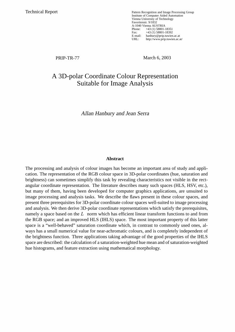
Figure 1: Example iso-brightness surfaces for two digital colour spaces in which the coordinatesare encoded using 8 bits. (a) HSV for K 4 B �

. (b) HLS for K 4�8!�.

For brightness K , one can visualise the iso-brightness surface by starting from the cube withprincipal diagonal between

���������)� and

� 8 K � 8 K � 8 K for K��� � � , or with principal diagonal be-

tween� 8 K�� �<� 8 K�� �<��8 K�� �C

and�'�<���<���C

for K�� � � � . The iso-brightness surface consists of thesix triangles inside the cube with edges formed by the lines between the point

� K � K � K and thesix vertices of the cube which are not on the achromatic axis. An example of this iso-brightnesssurface is shown in figure 1b. The projection of this surface onto the chromatic plane also re-sults in a hexagon, except that for this model, the largest hexagon is found at K 4 � � � . The solidproduced by stacking these hexagons is therefore a double-hexcone. A vertical slice along theachromatic axis through the HLS colour space is shown in figure 10c.

For the HLS model, the hue calculated as for the HSV model (equation 4), and the com-monly used saturation expression is

�=FG� 4 789 8:� ,-, #.� �����������54 J,./ ����������������A����� ��� �� !#�%$'&��>��� ��� �� �����A����� ��� �� ����%$'&��>��� ��� �� ,-, ���=F�� �

�������(�)��� ��� �� @!#�%$'&A����� ��� �� � !� �����(�)��� ��� �� ���%$'&A����� ��� �� �� 1 $32�(�* " , &%( (6)

2.3 Problems arising when using these spaces for image analysis

The HSV and HLS colour spaces were developed during the 1970’s for easy numerical spec-ification of colours in computer graphics applications [26]. In this context, the hexcone anddouble-hexcone shapes of the spaces are inconvenient, as it would be easy for a user to acciden-tally specify coordinates which lie outside the colour gamut. As computers of the time were notvery speedy, additional checking to avoid this would have been unacceptable, so the solution ofexpanding the colour spaces into cylindrical form was adopted. This is easily done by defining

4

the saturation as the ratio of the actual distance of a point from the achromatic axis to the max-imum distance for the corresponding brightness value. The HSV cone and HLS double-coneare thereby expanded into cylinders. Vertical slices through these cylinders are shown in fig-ures 10b for the HSV space, and 10d for the HLS space, to be compared with the slices throughthe conic and bi-conic versions of the spaces in figures 10a and 10c respectively. Indeed, thecommonly used saturation expressions (equations 3 and 6) describe such cylindrically shapedspaces. The dependence of these saturation measures on the corresponding brightness is easilyseen. For example, given the definition of brightness in the HSV space, the first level of theHSV saturation expression (equation 3) can easily be rewritten as

� � , / �2���)�J��������� �213 (7)

The HLS saturation can also easily be rewritten in terms of� �=FG�

. These cylindrically shapedcolour spaces have unfortunately been adopted by the image analysis community (and imple-mented in image analysis software2), leading to the widespread use of an unsuitable definitionof saturation.

To demonstrate the unsuitability of the cylindrically shaped spaces for image processing andanalysis, we use the colour image in figure 11a. This image was captured under slightly non-uniform lighting conditions, so that not all the pixels which look white have RGB coordinates ofexactly

�E�<���<���C. The upper part of the image was then inverted by subtracting the values in each

of the�

,�

and�

channels from the maximum possible values (i.e.8<B+B

for this � -bit image).The HSV saturation image calculated from this colour image is shown in figure 2b. The lowerpart of this saturation image, corresponding to the white region in the initial colour image, hasa saturation of around zero, as expected. However, some of the black pixels in the upper partof the colour image are shown as being fully saturated. This patently contradicts the definitionof saturation, which states that saturation should be low for almost-achromatic colours, andzero for greylevels. The reason is that some of the black pixels have small non-zero

�,�

or�components. The expansion of the HSV cone into a cylinder (demonstrated in figures 10a

and b) results in these pixels getting artificially high saturation values. One therefore has theridiculous situation where some of the black pixels are shown as being more highly saturatedthan the colourful regions that they surround. Because of the double-cone shape of the HLScolour space, its expansion into a cylinder produces spurious high values of saturation in boththe high and low brightness regions, as shown in figure 2c. This is particularly noticeable forthe orange region at the bottom of the image, on which two of the white letters are shown ashaving saturation values equal to the surrounding orange colour.

This demonstrates that two of the common assumptions about these models are not truewhen the cylindrically shaped versions are used:

1. Saturation is defined as the chromaticity of a colour, so that pixels which appear black,white or grey should have a lower saturation than colourful pixels. As was shown in theexample above, pixels which appear black or white often have maximal saturation valueswhen one of the cylindrically shaped spaces is used.

2Software already used by the author which implement cylindrically shaped colour models include: Matlabrelease 12.1, Aphelion 3.0, Optimas 6.1 and Paint Shop Pro 7.

5

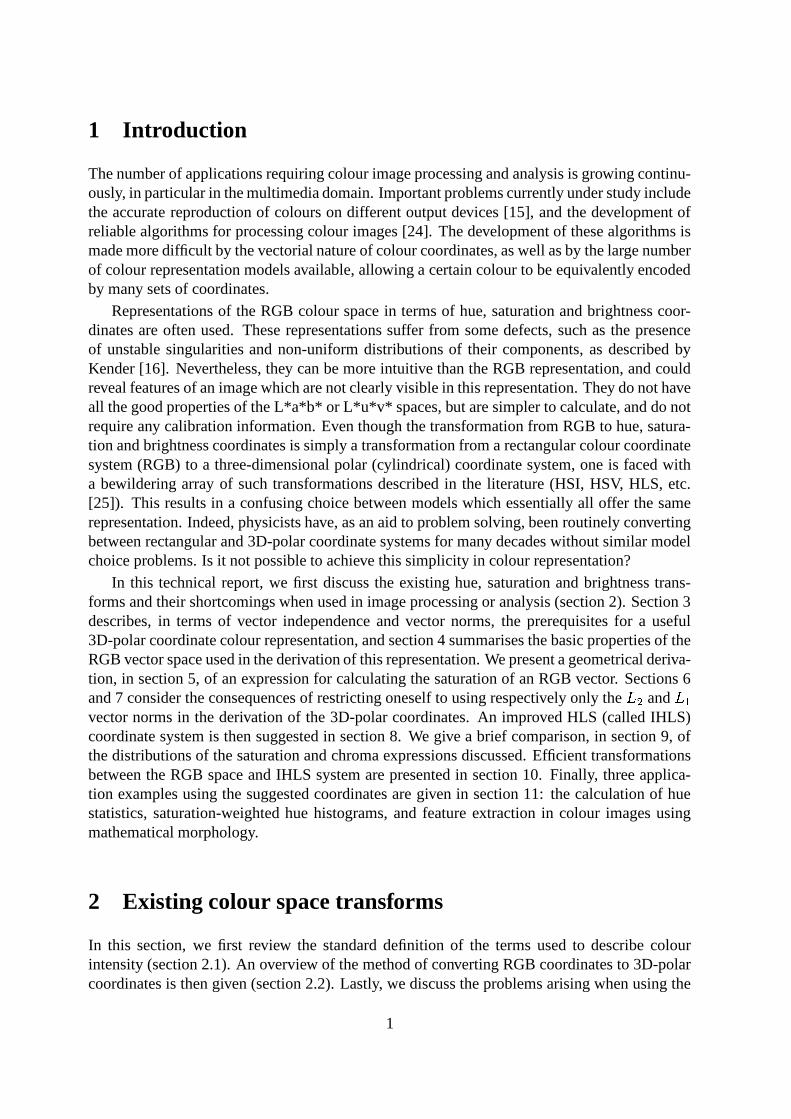
(a) Luminance (b) HSV model saturation

(c) HLS model saturation (d) Suggested saturation definition

Figure 2: 3D-polar coordinate components of figure 11: (a) Luminance. (b) HSV model satu-ration. (c) HLS model saturation. (d) The suggested saturation measure.

2. It is often said that these spaces separate chrominance (hue and saturation) and brightnessinformation. However, use is made of the brightness function to normalise the saturationin the cylindrically shaped spaces (as shown in equation 7). It is clear that the saturationvalues therefore depend critically on the brightness function chosen (demonstrated by thelarge differences between figures 2b and c).

We now consider two cases of the confusion that the cylindrical forms of the colour spacescan cause. Demarty and Beucher [7] applied a constant saturation threshold in the cylindricallyshaped HLS space (figure 10d) to differentiate between chromatic and achromatic colours. Thisthreshold can be represented by a vertical line on either side of the achromatic axis in figure 10d,and it is clear that this does not correspond to a constant saturation. Demarty [6] later improvedthe threshold by using a hyperbola in the cylindrical HSV space (figure 10b), which correspondsto a constant threshold in the conic HSV space (figure 10a). Smith [27] makes the assumptionthat the cylindrical HSV space is perceptually uniform when a Euclidean metric is used, butupon examining figure 10b, one sees that a certain distance in the high brightness (top) part ofthe space corresponds to a far larger perceived change in colour than the same distance in thelow brightness part of the space. Such an assumption is almost certainly truer in the conicallyshaped version of the space. This problem also affects the quantisations of the cylindrical HSV

6

space in which an equal number of saturation bins are used in the high and low brightnessregions of the HSV space. Almost imperceptible colour changes in the low-brightness regionare quantised into the same number of bins as highly-visible changes in the high-brightnessregion.

2.4 Removal of the brightness dependence of the saturation expression

The simplest way of avoiding the disadvantages tied to the cylindrically shaped spaces is toremove the brightness normalisation from the saturation expressions, hence reverting to theoriginal shapes of the spaces. Removing this brightness dependence from the saturation for theHSV model is simply done by multiplying equation 3 by the brightness

�����, giving ���� 4 #�� �������J�)� � J,./ �2���)�J���� (8)

where the superscript ‘NC’ indicates that this is the non-cylindrical version. For the HLS space,removing the brightness dependence is slightly more complex due to its double-cone shape.The non-cylindrical saturation is �����=F�� 4 � F�� � � � 8����� �8 � � � F�� ������ (9)

which after some manipulation also reduces to equation 8. The equivalence of these non-cylindrical saturation expressions is tantalising, and we show that it is in fact derivable fromthe basic definition of saturation in section 5.

3 Vectors, norms and independence

We now define clearly what the notions of vector space, norm and independence contribute tocolour image representations. In the following, the RGB space is modeled by the Euclideanspace � , with its projections, orthogonality, etc., but we equip it successively with differentnorms, including amongst them the Euclidean norm.

The vector space notion associates a point1�4 �����������

to the vector �� �� . It defines:� The sum of a number of vectors as being the vector made up of the sum of the vectorcomponents.� The product of a vector and a scalar as being obtained by multiplying each component ofthe vector by the scalar.

Note that these operations transform vectors into vectors, and not into numbers. We knowthat every vector can be uniquely written in terms of its components for each system of axes.Therefore, starting from the unit cube with coordinates

� � � � �,� � � � �

and� � � � �

,we define the diagonal between

�����������<and

�E�<���<���Cas the achromatic axis, and the plane

intersecting the origin and perpendicular to this axis as the chromatic plane, which containsall information on the colour. Hence, the point

1can be written as �� �� 4 �� �� = �� �� = �� ��

, orequivalently as �� �� 4 �� ���� = �� ���� , where

1 �and

1 �are the projections of

1onto respectively the

achromatic axis and the chromatic plane.

7

Can we therefore say that the vectors1 �

and1 �

, which are orthogonal, are also independent?The response depends on the meaning which we attribute to the adjective “independent”. If werefer to a possible link between the two projections

1 �and

1 �, they are obviously not indepen-

dent: the points of low brightness always have low colour saturation. But the independence canalso signify something else, for example that the parameters that we associate with

1 �(satura-

tion, hue) don’t affect those associated with1 �

. In this case, if two differently coloured points1and

1 5have the same projection

1 �, they have the same saturation and the same hue. In order

to have a colour representation adapted to image analysis, we therefore propose the followingprerequisite:

First prerequisite: Two distinct points which have the same projection onto the chromaticplane, have the same chromatic parameters.

We could go further and require that two points which have the same projection onto theachromatic axis have the same intensity. However, this would limit one to symmetric functionsof�

,�

and�

, excluding notably weighted expressions such as the luminance (equation 1).Another useful concept on which we now base our discussion is that of the norm. It asso-

ciates a parameter, which we call � , with every vector. This parameter is zero or positive, and itsmagnitude becomes larger as point

�moves further away from the origin, i.e. � ��� 13�4�� � �213 ,

in which��� �

is a weighting factor. Furthermore, the norm links the addition of vectors to thatof numbers by the classic triangular inequality

� �21 =?1 5 ��� ��13 = � ��1 5 (10)

which says that the norm of the mean vector between1

and1 5

cannot be larger than the averageof the norms of

1and of

1 5. For example, two projections onto the chromatic plane which are far

from the achromatic axis, but opposite each other, represent colours which are highly saturated.The vector mean of these two colours is, however, achromatic. It therefore makes sense that itsnorm should not be larger than the norms of the original colours, and hence that the inequalityof equation 10 should be satisfied. Lastly, it is equivalent to say that the vector

1is zero or that

its norm is zero 1 4�� � ��13 4F�(11)

When this last condition is not satisfied, we refer to a semi-norm. We note that in the triangularinequality 10 the two ‘+’ symbols do not have the same meaning: the first is with respectto vectors, and the second with respect to numbers. The same is true for the two zeros inequation 11.

We will consider in more detail the norms���

and� �

, and the semi-norm #.� � , / (proofthat it is a semi-norm is given in appendix B). Use of the

� �norm leads to conversion formulae

which are quadratic and rather difficult to invert. Conversely, the distance associated with thisnorm is the Euclidean distance, which is well-known and convenient to work with.

The� �

norm has already made its appearance in colour space conversions, but withoutannouncing itself as such. We see it for example in [3] and [9] for the achromatic axis, andin the standard triangle colour model [17]. Its associated distance is less intuitive than theEuclidean distance, but faster to implement and usually just as precise. We note lastly that,given variables

���)�J����� �, every quantity � � =� � =�� �

, with weights � �� 5����� �is still

an� �

norm on the achromatic axis. This leads to the second prerequisite:

8

Second prerequisite: The brightness parameters associated with colour vector1

and with itsprojection

1 �must be norms.

In addition to the two prerequisites already mentioned, it is convenient to introduce a thirdconstraint, less fundamental and suggested by practical experience. It is extremely convenientif one is able to return to an RGB space image representation at the end of an image processingtask, which leads us to propose the third prerequisite:

Third prerequisite: Every system for the representation of colour images must be reversiblewith respect to the RGB standard.

If we examine the HLS system in the light of the first two prerequisites, the basic reasons forthe criticisms presented in section 2.3 become clear. In the HLS system, neither the saturationnor the brightness are norms, and in addition, there is no independence between the achromaticaxis and the chromatic plane: it’s almost impossible to develop a worse colour space.

One can show the lack of independence by considering the points1G4 � � ��� � � ��� �)� and1 5 4 � � � � � � � � � � ��� , which both project onto the same point

1 �on the chromatic plane. Their

HLS saturations are given by �����=! �%$'&����� ���%$'& as their brightness values are �� � � . The first has an HLS

saturation of�

and the second of� � (the latter point has a smaller saturation as its brightness

value is higher than that of the other, we once again come across a problem in the commonlyused cylindrical form). Not only does this representation create artificial differences betweenpoints, but it fails to discriminate between points which are different: all points with brightness�� � � and with J,./ 46�

have the same saturation.To show that the brightness

� 4 ����� � �%$'&� does not satisfy the triangular inequality, we canuse the points

1�4I� � � � � � � � ��� and1 5 4I�2��� � � � � � � � , both having HLS brightness values equal to� ��� , while the brightness of

1 = 1 5is equal to ��� . Finally, the HLS saturation is not a norm either,

as the points1�4 � � � � � � � � � and

1 5 4 � � � � � � � � � both have saturation of� � while their sum

has a value of�

(the term #�� � J,./ , on the other hand, stays the same).

4 Properties of the space under consideration

In the RGB unit cube, the achromatic axis is placed between the points�2���������

and�'�<���+���C

,and contains the colours for which

�F4F� 4��. The chromatic information is entirely encoded

in the chromatic plane, perpendicular to the achromatic axis and intersecting it at the origin.Every vector

1of the RGB unit cube is decomposed into the vectorial sum of its projections

1 �onto the achromatic axis and

1 �onto the chromatic plane

1�461 � = 1 �(12)

in which all chromatic information is encoded in the vector1 �

. We adopt the notation in whichall the vectors projected onto the chromatic plane take a subscript � . Hence �

�and �

�represent

respectively the projections onto the chromatic plane of the pure red vector � and pure greenvector � .

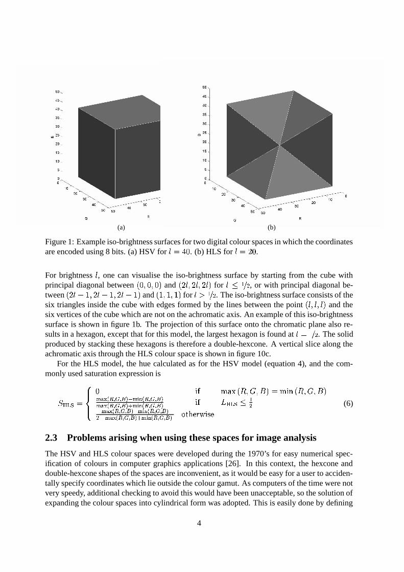
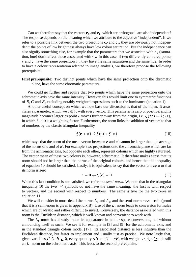
The chromatic plane is shown in figure 3a, and we proceed to draw the reader’s attentionto some of the important features shown in this figure. The hexagon surrounds the regions intowhich points in the RGB cube are projected, and the circle circumscribing the hexagon has

9

o

r

ma

b

cy

g

y

z

θ

p

p

p

p

p

p

π/6

π/3

vp xp p

cp

(a)

Smax

H

60°

(0,0,0)

63

120°− Hr ypp

(b)

Figure 3: (a) The chromatic plane. (b) The red-yellow sector of the hexagon on the chromaticplane. The lower vertices correspond to the colours red (at the left) and yellow. The angle

4takes values between

� Cand

;<� C.

a radius of� � . If we limit the points projected onto the plane to only those with a specific

brightness, then the hexagon has an area smaller than or equal to the one shown. A point1

projected onto the chromatic plane has coordinates

1 � 4 � � 8!� � � � ��� � �28+� � � � � � � � 8+� � � � � � � (13)

The projections onto the chromatic plane of pure red �4 �E�<�����)�

, yellow � 4 �E�<���<�)� and

green �4I�2�����<���

have coordinates

�� 4�� 8� � � �� � � ���� � � � 4�� �� � �� � � 8�� � � � 4� � �� � 8� � � ��� (14)

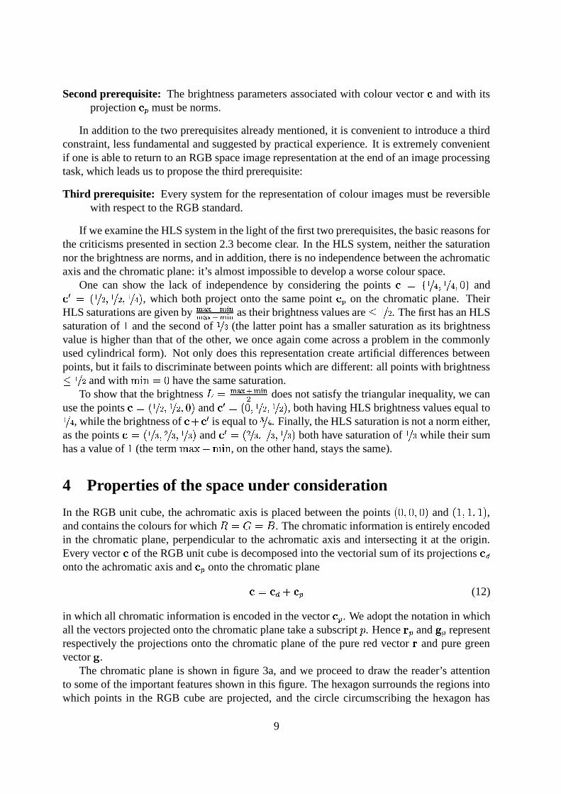
The RGB unit cube is shown in figure 4. We point out some useful correspondences betweenregions of the cube and their projections onto the chromatic plane. Points for which

��� �form

the half-space limited by the plane � ��� which contains � in figure 4. Its points are projectedonto the half-plane limited by � ��� � and containing �

�in figure 3a. Similarly, the points for

which� �F�

form the half-space limited by � � ��1 � which contains � (figure 4), with pointsprojected onto the half-plane limited by �

� �21 � � and containing ��. Lastly, the points such that� =D� � 8+� 4 �

form the plane passing through the achromatic axis and the line� = � 4 �

in the plane � � � . This plane cuts the chromatic plane along the line parallel to ���� �

passingthrough � .

With respect to colour, the RGB cube is divided into six sectors delimited by the six planeseach containing the achromatic axis and one of the three

�,�

and�

axes or one of the diagonals

10

r y

=(1,1,1)

1

2

3

4

5

0

=(0,0,0)o

w

g

cyb

ma

xv

z

c

R

B

G

Figure 4: The RGB unit cube. The italic numbers indicate the edges corresponding to the sixsectors into which the RGB cube is divided.

in the squares in� 4 �

,� 4 �

or� 4 �

. The following equation gives the sector of a colourbased on the order of magnitudes of the RGB coordinates

����1354 78888889 888888:

� ,-, � � ���6�� ,-, � � � � �8 ,-, � � � ���� ,-, � � � � �B ,-, � � ��� �B ,-, ��� � � �

(15)

The cube edge corresponding to each sector is indicated by the italic numbers in figure 4.We now assign a polar coordinate system to the chromatic plane, taking the vector �

�as the

origin of the angles. The angular values increase as one moves in an anti-clockwise direction.Every point (i.e. every vector)

1of the RGB unit cube can be equivalently written in terms of

RGB Cartesian coordinates, or 3D-polar coordinates��� 1 � � ����1 � � ���<

.One nevertheless has different equations for converting from one system to the other de-

pending on whether one uses the� �

or� �

norm. For the� �

norm

� 1�� � 4�� ��� � =����� � =�� �� �(16)

and for the� �

norm, one has � 1 � 4 � � � = � � � = � � �(17)

The differences are large enough that we study more precisely, in sections 6 and 7, the advan-tages and disadvantages of the two approaches.

11

Finally, for the semi-norm �4 #.� � , / , we find for vector

1 4 �����������and its

chromatic projection1 �

of equation 13,

��213 4

��21 � 4 #.� �2��������� � J,./ �2��������� (18)

which means that this semi-norm is exclusively chromatic (it does not see variations in thebrightness).

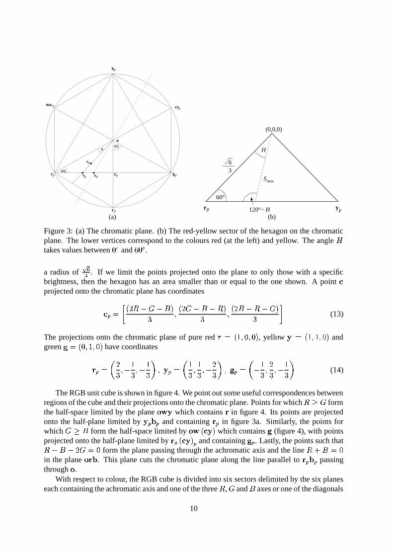
5 Geometric derivation of a saturation term

The saturation and chroma measurements are associated with the length of the vector1 �

. Theirdefinitions are:

Chroma: The norm of1 �

is used, as done by Carron [2] (who uses the� �

norm). It assumesits maximum value at the six corners of the hexagon projected onto the chromatic plane.The shape of the resultant space obtained by piling up the hexagons is a hexcone ordouble-hexcone.

Saturation: For the saturation, the hexagon projected onto the chromatic plane is slightly de-formed into a circle by a normalisation factor, so that the saturation assumes its maximumvalue for all points with projections on the edges of the hexagon. The shape of the resul-tant space is therefore a cone or double-cone. Poor choice of this normalisation factor hasled to some of the less than useful saturation definitions currently in use.

We now geometrically derive a saturation coordinate which does not suffer from the disad-vantages enumerated in section 2.3 and is therefore much more useful in image processing andanalysis. This derivation is based on the one for the Levkowitz and Herman GLHS model [17].

5.1 Basic saturation formulation

To calculate the saturation of a colour represented by a vector1

in the RGB space, we beginby considering the triangle which contains all the colours which have the same hue as

1(iso-

hue triangle), shown in figure 5a. The achromatic axis always forms one of the sides of thistriangle. The vector �

�213 4 K ��13 � K ��13 � K �213 � gives the position on the achromatic axis inRGB coordinates of the brightness value associated with

1. The iso-brightness line associated

with1

is the intersection of the iso-hue triangle and K �213 iso-brightness surface, and hencepasses through �

�213and

1. By definition, all the iso-brightness lines in the triangle are parallel.

The point with the same hue as1

lying furthest away from the achromatic axis is labeled ���13

.This point necessarily lies on one of the edges of the RGB cube.

Traditionally, the saturation is defined as the fraction given by the length of the vector from��213

to1, divided by the length of the extension of this vector to the surface of the RGB

cube. This definition produces a space in the form of a cylinder. We call this type of saturationa cylindrical saturation. The problems inherent in the use of this saturation definition havealready been described in section 2.3.

In order to keep the conical form of the space, it is necessary to change the definition ofthe saturation. In figure 5a, instead of dividing the length of the vector from �

�213to1

by

12

( )c

( )c

( )c(0,0,0)

(1,1,1)

cL

q

q L[ ]

G

B

R(a)

( )c

( )c

L

r y

=(1,1,1)

h

c

q

cq

=(0,0,0)b

w

B

R

G

(b)

Figure 5: (a) Diagram used in the derivation of a general saturation expression. (b) Diagramused in the derivation of the simpler saturation expression. Both diagrams show the trianglewhich contains all the points with the same hue as

1.

the length of its extension to the edge of the cube, we divide it by the length of the vectorbetween �

��213 �

and �� 13

. This is the longest vector parallel to the iso-brightness lines, whichnecessarily intersects the third vertex �

�213of the triangle. We therefore have the following

general definition of saturation 4 ����13 � 1��

��

���13 � � �

�213 � (19)

which gives the natural conic or bi-conic form to the 3D-polar coordinate colour space, andwhich additionally is independent of the choice of the brightness function. A proof of thisindependence is presented in appendix A. This saturation calculated for figure 11a is shownin figure 2d. It is clear that the defects associated with the cylindrically shaped HSV and HLSmodels are not present. The colourful regions always have saturation values higher than thesurrounding monochromatic background. Furthermore, one would obtain the same saturationvalues irrespective of the brightness function used.

5.2 A simple expression for the saturation

In this section, we use equation 19 to derive a very simple saturation expression. For this deriva-tion, we choose the iso-brightness surfaces to be parallel to the nearest side of the RGB cubewhich intersects the origin (which we are free to do due to the independence of the brightnessand saturation). This is the

� 4F�plane for sectors

�and

�, the

�F46�plane for sectors

8and

�,

and the� 4��

plane for sectorsB

andB. The brightness function producing such iso-brightness

surfaces is� ��13 4 , / �2���)�J���� (20)

13

At first, we consider only sector�, which contains point

1 4 �2���������as shown in figure 5b.

The brightness vector of1

is ��213 4 �2� �)� ���

, due to1

being in sector�. We project

1onto

the� 4F�

plane resulting in point1 � which is the same distance from the origin as �

�213is from1

. The coordinates of1 � are therefore

�2� � � ��� � � ��� . We then construct the line between�

and1 � in the

� 4 �plane parallel to the cube edge between � and � , forming two similar

triangles with vertices � ,�

and1 � , and � , � and �

� 13. The following relation is therefore valid:

� � � 1 � �� � � ��213 � 4

� � � � �� � � �

� (21)

The term on the left is simply the definition of saturation given by equation 19. On the right,� � � �� 4 �

, and as the coordinates of�

are�2� � � �����)�

,� � � � � 4 � � �

. Hence thesaturation

4F� � �, which in sector

�, is equivalent to �� 4 #.� �2��������� � J,./ �2��������� (22)

The derivation is easily done for the other five sectors to show that equation 22 is valid forthem all. The simple saturation expression obtained for the non-cylindrically shaped HSV andHLS spaces (section 2.4), is therefore obtained from the general saturation definition. The #.� � J,./ expression is in fact a semi-norm, as proved in appendix B. We return to thissaturation expression in section 8, in which we suggest an improved version of the HLS space.We first consider the consequences of strictly imposing either the

� �or� �

norm on the RGBspace.

6 The framework of the� 8 norm

We expect this norm to be the best adapted to the problem, as it is based on the Pythagoreantheorem, which interprets the norm in terms of vector lengths. In addition, the scalar productwhich accompanies it is an indispensable tool for calculating angles.

The conversion equations from the RGB coordinate system are easy to determine. We callthe norms of the vectors projected onto the achromatic axis and the chromatic plane respectively� �

and � � , both these norms being scaled to the range ��������

. The angle�

is called4 �

. By usingrelation 16 and figure 3a, the following can be derived

� � 4 �� �� � � =?� � =?� �� � � �(23)

� � 4 � � 8 � 1 � � (24)

4 � � � =?� � =>� � � � � � � � � ��������(25)

Note that � � is a measurement of the chroma, as it is simply the norm of1 �

multiplied by aconstant. We can convert this chroma into a saturation by applying equation 19 in the chromaticplane, where it is equivalent to � 4 � 1 � � ����� (26)

14

in which ����� is the distance from the origin to the edge of the hexagon for a given hue

4, that

is, the maximum value that can be taken by the norm of a projected vector� 1 � �

with hue4

.The red-yellow sector of this hexagon is reproduced in figure 3b, in which the upper vertex isat the origin

�2��������� , the lower left vertex is the projected red vector �

�, and the third vertex the

projected yellow vector � � . It is simple to show using figure 3b that ����� 4 � 88 &%, / �'�C8!� C � 4 (27)

for� C � 4�� ;<� C

. To make this equation valid for the values of4 �? �� C � � ;<� C

, it is sufficientto replace the

4in the equation by4�� 4 4 ��� � ;<� C where � � � �����<��8�� � � B � B � & 1 $32 # $ � C � 4�� � ;<� C

(28)

Note that this saturation expression (equation 26) gives exactly the same values as the #.� � J,./expression, as they are both derived from the same definition.

The calculation of the angle�

in figure 3a is done in terms of the scalar product between thevectors

1 �and �

�as

� 4 #+*%��� 1 & � ���� 1 �

��� � � 1 � � � (29)

4 #+*%��� 1 & � � ���� �

���

�2� � =?� � =>� � � � � � � � � ��� �� (30)

in which ���� 1 �

indicates the scalar product of the two vectors. The possible values for�

arebetween

� Cand

���DC

, and it is therefore necessary to expand this range of values by using4 � 4 � � ;<� C � � , , � � �� 1 $ 2-(�*'" ,.& ( (31)

Formally, the problem is solved. The variables� �

, � � , � and4 �

are expressed in termsof�

,�

and�

. Nevertheless, irrespective of the theoretical equivalence of the two systems,the inverse transformation is not simple. It is desirable to simplify this pure

� �norm system

either by using another norm, which is considered in the next section, or by using a mixture ofdifferent norms, discussed in section 8.

7 The framework of the� � norm

In this section, we continue to use the same vector space, with the decomposition1�4�1 � =>1 �

,but we assign the

� �norm to the vectors of the space.

7.1 Brightness and chroma

Because the�

,�

and�

coordinates are greater than or equal to zero, the� �

norm (equation 17)of the vector

1 �is simply the sum of the

�,�

and�

components. As we wish the value of thebrightness to be in the range

��������, we take it to be the arithmetic mean of the components of

1� � 4 �� ��� =>� =?�

(32)

15

We note that if two points1

and1 5

have the same projection1 �

on the achromatic axis, we have� 1 1 5 � 4��, and by application of the triangular inequality one finds that

� � ��13 4 � � �21 5 .

The chroma � � is defined as being proportional to the� �

norm of the vector1 �

, that is

� � 4 �B � 8+� � � � � � = � 8+� � � � � � = � 8!� � � � � � �(33)

The constant ensures that the chroma values lie in the range ��������

, as the expression within theparentheses has a maximum value of

Bobtained when two of the components have an extremal

value, and the third has the opposite extremal value. The saturation is zero when� 4 � 4G�

,i.e. when the point

1lies on the achromatic axis.

In order to remove the absolute values, linked to the choice of the� �

norm, from equa-tion 33, it is necessary to find the maximum, median and minimum of

�2���������, which we

denote as #.� , , � and , / . As equation 33 is symmetric in terms of�

,�

and�

, it issufficient to adopt a convention, for example

� � � � � � � � �(34)

and, in the calculation, to replace�

by #�� ,�

by , � and�

by J,./ . When the componentorder in relation 34 is true, the first term of equation 33 is positive and the third is negative. Thesecond term, which has a variable sign, distinguishes between two cases:

1. if�F=>� �68+�

, or equivalently� � � �

, then

� � 4 �8 �2� � �H =F�2� � � � 4 � 8 �2� � � �

(35)

2. if�F=>� � 8+�

, or equivalently� � � �

, then

� � 4 �8 �2� � � =F��� � � � 4 � 8 � � � � �

(36)

For��=?�F4F8+�

, we find for both forms:

#.� � J,./ 4F� � � 4 B � � � (37)

The hue, being an angle, is calculated in the same way as for the� �

norm, using equations 30and 31.

In summary, despite the presence of two cases for the saturation, the transformation equa-tions 32, 35 and 36 make up a linear system much simpler than in the case of the

� �norm. The

hue calculation is the most complex, and we now develop an approximation of the trigonometrichue.

7.2 Simplified calculation of the hue in the ��� space

The following approximation is largely based on the approach presented in [17]. Firstly, welimit ourselves to vectors having

� � � �6�and non-zero chroma. Their projections onto the

chromatic plane form the triangle � � � � � in figure 3a. Because the hue origin is the vector ��, the

16

angle�

in figure 3a varies from�

to � /3 in radians, or conventionally from�

to�. To approximate�

, we begin with the hue-fraction equation in the HLS system, that is4 4 ��!=�������! �%$'& , and we

transpose it mutatis mutandis, that is to say by replacing #���� J,./ , which corresponds tothe saturation in the HLS system, by our corresponding

� �norm chroma expression (differing

only by a factor) and taking into account the duality of the two chroma expressions. Moreprecisely, because the line �

���

is parallel to the line � � in the� 4 �

plane, when�

variesfrom

�to�, the point � of the

��4 �plane describes the half-diagonal ��� , and its projection� � describes the segment �

� � � of the chromatic plane. The point � , the intersection of the plane�D= �F= 8+� 4 �(which contains the achromatic axis) and the line � � , divides the two zones

having different chroma definitions. In the projection, the point � 4 � � � � � � ��� gives the point� � , which corresponds to the value

� 4 � � � .As the value #.� � , / of the HLS system corresponds to the saturation, we replace it here

by the� �

norm chroma � �� 4 �� � �2� � � � " , $32 �?=?� ��8+�

(38)

We have � 46�for �

4 �'�<������� . The factor � is determined by the condition of having � 4 � � � at

� 4 � � � � � � ��� , which gives � 4 ��� . When�?=?� � 8+�

, the duality suggests the replacementof� � �

by� � �

, and � by� � � , or

� 4 � ��B � � �

� � � " , $32 � =>� � 8+�H(39)

In fact, at point � � , the chroma � � takes the same value of�/�

in the two modes, and we find� 4 � � � . Finally, at the extremity of the range of�, we see by using point � or point � , that� 4 �

.We can reduce equations 38 and 39 which define � to a single equation by making use of

the critical element� =?� � 8+�

. We find��=?� � 8+�G4 � � �'� � 8 � (40)

which demonstrates the equivalence relations��=>� � 8+� � ��� � � � �

�8 (41)

��=>� � 8+� � ��� �8 � � � �

(42)

A simple numerical experiment has shown that the maximum difference between this hue ap-proximation � and the trigonometric hue is the same as for the approximation suggested in [17],that is

�<7 �:8 C.

7.3 Colour space conversions in the � � space

The preceding results lead to the following conversion formulae for the conversion����������� �� � � � � � � �

7889 88:� � 4 � �2�?=?� =>�� � 4 �

�� 8+� � � � �54 � ��� � � � ,-, �6=?� �68+�

� � 4 ���2�?=?� � 8+�� 4 � � � � � � , , ��=?� � 8!�

� 4 �� � � �*�*! � ���� �

(43)

17

When��=?� ��8+�

, or equivalently, when� � � �

� � � , the transformation is inverted as

79 :�F4 � � = � � ��G4 � � � � � � = � � � �� 4 � � � � � � � � � � � (44)

and for��=?� � 8!�

(or� � � � � � �C

as

79 :�F4 � � = � � � � � � �� 4 � � � � � � = � � � �� 4 � � � � � � (45)

The domain on which the equations are defined� �F� �6� ��� ���

(without the achromaticaxis) corresponds to the tetrahedron � � ��� in the figure 4. The coefficients of system 43 werechosen so that

� �, � � and � vary between

�and

�, which does not necessarily mean that

they always correspond to points inside the tetrahedron. The following equivalence relation isnevertheless easily verifiable

� � ��� � � � � ��� 8� � � � � � � � �8� � � (46)

In practice, this condition is not too limiting, as it is simple to prevent operators applied tovector

1, expressed as

� � � � � � � � from giving a result outside the RGB cube.The last case to study is that in which the vector

1lies on the achromatic axis, i.e. the case

for which� 4I� 4I�

. The system 43 is no longer valid, as we introduce a division by zero,and must be replaced by

79 :� � 4 � �2�?=?� =>�� � 4 �

�� 8+� � � � �� 4 �

����D=>� � 8+�

� � �E� � 8 � 4 �6=?� � 8+� (47)

which shows that � is indeterminate. This does not mean that it is impossible to find the colour1, but that the chromatic intensity � � �'� � 8 � is zero.

7.4 Conversions to the complete digital cube

We move from one sector of the RGB cube to another by adding to � the sector number givenby���213

of equation 15. The hue is therefore approximated by4 � 4 �����213 = � � (48)

of the same structure as in the HLS system. The coefficient � determines the working units:� 46;+�for degrees, and � 4 B 8

to get resulting values between�

and8<B+8

which fit into 8-bits.In parallel to the conversion from � to

4 �, it is convenient to rewrite the brightness and

saturation in terms of #.� , J,.� and , / functions, which leads to the replacement of system 43by � � 4 �� � #.� = J,.� = , / (49)

� � 4 � � � #.� � � � ,-, #.� = J,./ ��8 J,.� � � � � � J,./ ,-, #.� = J,./ � 8 J,.� (50)4 � 4 � � ��� 13 = �8 � #.� = , / � 8 , �8 � � � (51)

18

This system of equations is also valid for 8-bit RGB values, and the resulting coordinates areencodable on 8-bits if � 4 B 8

is used. It is important to notice that for8<B+;

discrete�

,�

and�input levels, � � takes values which are multiples of

�/�

(i.e.B��C8

discrete levels between�

and8+B+;). Care should therefore be taken when rounding off these values for an 8-bit representation.For the inverse transformation, the value of

4 �gives, via

�, the order of magnitude of

�,�

and�

and the value of � � . Based on whether � � is � � � � or� � � � , we use system 44 or 45

replacing�

,�

, and�

by the components ordered according to the value of�

, and replacing �by � � .

8 The ������� ��� semi-norm and an improved HLS space

We now return to the HLS system and suggest an improvement which overcomes the disadvan-tages linked to the classic saturation definition. We will refer to this space as the improved HLSor IHLS space. In fact, it is not necessary to modify the HLS space much in order that it becompatible with the three prerequisites. It is sufficient to pass from its cylindrical version tothe conic version, which is done by replacing the HLS saturation by the function #.� � , / .A proof that this quantity is a semi-norm is given in appendix B. We now briefly consider thethree components of the IHLS system.

8.1 Saturation

The semi-norm � 4 #.��� , / obviously satisfies the first prerequisite on the independence

of the projection onto the chromatic plane. Adding to point1

a vector parallel to the achromaticaxis simply reduces to adding the same constant to every component of the

�2���������vector,

which does not modify the value of #.� � J,./ . In particular, in the RGB space, the vector1

and its projection1 �

on the chromatic plane have the same value for #.� � , / .On the other hand, this semi-norm is not invariant by projection onto the achromatic axis,

in contrast to� �

and� �

. As the point1

approaches the achromatic axis, the value of �

getssmaller, becoming zero when

1is on the achromatic axis. The projection

1 �of the vector

1onto this axis always has a value of zero for the semi-norm

�. It is therefore impossible to

build a representation based only on this semi-norm, which is blind to brightness. However, wesee also that for all the vectors in the chromatic plane (and only for these vectors), the quantity #.� � J,./ becomes a norm. This is why we use it for the saturation, complementing it bytaking the

� �or� �

norm on the achromatic axis.

8.2 Brightness

The� �

and� �

norms, and #.� � , / semi-norm which we have studied all guarantee thefirst prerequisite on independence: two different points

1and

1 5having the same projection

1 �onto the chromatic plane have the same saturation and the same hue. As this property remainsvalid independent of the norm chosen on the achromatic axis, one can easily replace

� �in

equation 23, or� �

in equation 32 by some weighted mean�

(which is still a norm)� �2��������� 4 � � = �D= � � " 2�(�*%( � = = � 4 �(52)

19

or even by a non-linear estimator, provided that it is a norm. The hue circle remains the same,giving the same weighting to the three fundamental colours, as does the saturation, even if thisis not the case for the brightness which replaces

� �or� �

.

8.3 Hue

For the hue, we have developed an exact trigonometric expression, given by equations 30 and31, and a simpler approximate form given by equation 51. Both these hue formulations stillshow evenly spaced spurious high values in the hue histogram when one converts from an RGBspace containing discretely spaced values [16]. However, with the trigonometric hue formula-tion, it is easy to remove or reduce the height of these histogram spikes by calculating a huehistogram only for pixels having a saturation above a chosen threshold [10]. With the approxi-mation, removal of the spikes is more difficult. Due to the high speed of modern computers, itis highly recommended that the exact trigonometric form be used.

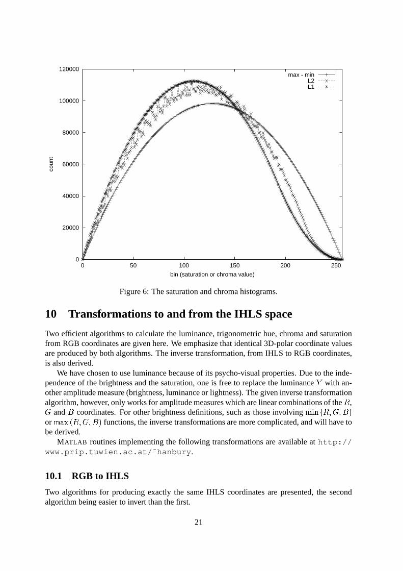
9 Comparison of the saturation and chroma formulations

We compare the distributions of three of the saturation and chroma formulations discussed inthis report: the #.� � , / saturation expression (equation 22), the

� �norm chroma (equa-

tion 24), and the� �

norm chroma (equation 50). These distributions are shown in figure 6.To calculate the distributions, we start with a

8<B+; � 8<B+; � 8<B!;RGB cube with a point at

each set of integer-valued coordinates. For the #�� � J,./ and� �

norms, the saturation (andchroma) values of each point are calculated (as floating point values), and then rounded to thenearest integer. Histograms showing the distribution of these integer values (256 levels) areshown in figure 6.

The� �

chroma measure has an inbuilt quantisation pitfall. When�

,�

and�

are integer-valued, then the

� �norm

� �is always a multiple of

�/ , and therefore #.� � � � and

� � � J,./in equation 50 are also multiples of

�/ . As both of these expressions are multiplied by /� when

calculating the chroma, � � is always a multiple of�/�

. In other words,�

,�

and�

valuesquantised into

8<B+;levels produce values of � � quantised into

B��C8levels. The rounding of a

floating point value of � � to the nearest integer therefore behaves extremely erratically, as the�/�

’s are sometimes rounded up and sometimes down, depending on whether their floating pointvalues are just above or just below

��7AB, thereby producing many spurious peaks and valleys in

the histogram. For the���

chroma distribution in figure 6, the values of � � were first multipliedby

8to get a series of integers between

�and

B��:8, and then adjacent pairs of histogram bins

were combined to produce the8<B+;

bin histogram shown.The #.� � J,./ saturation distribution is regular and symmetric around the central his-

togram bin because of the normalisation coefficient which deforms the hexagonally shapedsub-region of the chromatic plane into a circle. Conversely, the

� �chroma has a rather irregular

distribution due to the discrete space in which it is calculated. It also decreases very rapidly asone approaches higher chroma values because it is calculated in the hexagonally shaped sub-region of the chromatic plane. The

���norm chroma approximates the

� �chroma well (if the

quantisation effects are taken into account), and the histogram is more regular.

20

0

20000

40000

60000

80000

100000

120000

0 50 100 150 200 250

coun

t

bin (saturation or chroma value)

max - minL2L1

Figure 6: The saturation and chroma histograms.

10 Transformations to and from the IHLS space

Two efficient algorithms to calculate the luminance, trigonometric hue, chroma and saturationfrom RGB coordinates are given here. We emphasize that identical 3D-polar coordinate valuesare produced by both algorithms. The inverse transformation, from IHLS to RGB coordinates,is also derived.

We have chosen to use luminance because of its psycho-visual properties. Due to the inde-pendence of the brightness and the saturation, one is free to replace the luminance

0with an-

other amplitude measure (brightness, luminance or lightness). The given inverse transformationalgorithm, however, only works for amplitude measures which are linear combinations of the

�,�

and�

coordinates. For other brightness definitions, such as those involving , / �2���������or #.� �2��������� functions, the inverse transformations are more complicated, and will have tobe derived.

MATLAB routines implementing the following transformations are available at http://www.prip.tuwien.ac.at/˜hanbury.

10.1 RGB to IHLS

Two algorithms for producing exactly the same IHLS coordinates are presented, the secondalgorithm being easier to invert than the first.

21

10.1.1 The simplest implementation

For the simplest implementation, one calculates an amplitude measure (equation 1, 2, or 5), thesaturation using equation 22, and the hue using equations 30 and 31. We have therefore usedan� �

norm for the luminance, the #.� � J,./ norm for the saturation, and the scalar productof the

� �norm for the hue.

0 ��13 4 ��798 �C8+;<�>=?��79@��:B<8+�D=>��7 � @<8<8+�(53) ��13 4 #.� �2���)�J���� � , / �2���)�J���� (54)4 5 ��13 4 #+*%��� 1 & � � �

��� �

���

�2� � =?� � =>� � � � � � � � � ���H �� (55)

4 ��13 4 � � ;<� C � 4 5 ,-, � � �4 5 1 $ 2-(�*'" ,.&%( (56)

10.1.2 An alternative

An alternative way of arriving at exactly the same IHLS values is now presented. It is basedon the algorithm suggested by Carron [2]. The changes with respect to Carron’s version arethe extension to calculate the saturation from the chroma, and the use of luminance instead ofbrightness. It is also similar to the IHS system described by Pratt [23], except for a change inthe hue origin and a different saturation definition. It still uses the

� �norm luminance expres-

sion, but an� �

norm for the saturation. This algorithm allows a more straightforward inversetransformation to be derived as it contains no #.� or , / functions.

The first step is to calculate the luminance0

and two chrominance coordinates�� 0� �� ���4�� ��7A8��C8<B ��7A@��CB B ��7A� @+8��

� ��� �

��� �

� � � ������ �

����

(57)

followed by the calculation of the chroma � �I ��������(this chroma is equal to the chroma � �

derived in the framework of the� �

norm in section 6)

� 4�� � �� = � �� (58)

and the hue4 � �� C�� � ;<�DCE�

4 4 79 :undefined ,-, � 4��#+*%��� 1 & � � �� � ,-, � /46� #+/-� � � � �� ;<� C � #+* ��� 1 & � � �� � ,-, � /46� #+/-��� � � � (59)

We derive from equations 24, 26 and 27 the value of the saturation � ��������

4 8 � & ,./ �'�:8+� C � 4 � � � (60)

in which 4 � 4 4 ��� � ;<� C where � � � �����<��8�� � � B � B � & 1 $32 # $ � C � 4 � � ;<� C(61)

22

10.2 Inverse transformation from IHLS to RGB

To transform colours represented in the IHLS coordinate system obtained using either of thealgorithms of section 10.1 to RGB coordinates, one first calculates the chroma values from thesaturation values (using equation 60)

� 4 � � 8 &%, / �'�C8+� C � 4 � (62)

where4 �

is given by equation 61. From the chroma, one calculates

� � 4 � � 1 & � 4 (63)� � 4 � � & ,./ � 4 (64)

For the case where the hue is undefined: � � 4 � � 4 �. Finally, the inverse of the matrix used

in equation 57 is used to obtain�

,�

and�

�� �����4�� �+7A�<�+�<� ��7A@

�@<B ��7 � @�� B�+7A�<�+�<� � ��7A8��C8+B � ��7A8+� B���+7A�<�+�<� � ��7A8��C8+B ��7�� B

� �

�� �� 0� �� ���

(65)

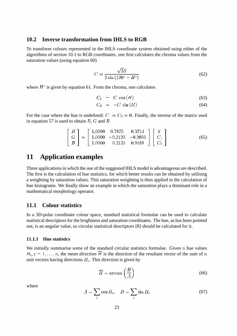
11 Application examples

Three applications in which the use of the suggested IHLS model is advantageous are described.The first is the calculation of hue statistics, for which better results can be obtained by utilisinga weighting by saturation values. This saturation weighting is then applied in the calculation ofhue histograms. We finally show an example in which the saturation plays a dominant role in amathematical morphology operator.

11.1 Colour statistics

In a 3D-polar coordinate colour space, standard statistical formulae can be used to calculatestatistical descriptors for the brightness and saturation coordinates. The hue, as has been pointedout, is an angular value, so circular statistical descriptors [8] should be calculated for it.

11.1.1 Hue statistics

We initially summarise some of the standard circular statistics formulae. Given � hue values4�� ��� 4 �<��7�7�7�� � , the mean direction4

is the direction of the resultant vector of the sum of �unit vectors having directions

4��. This direction is given by4 4 #+*%� $�#+/ � � � (66)

where 4�� � 1 & 4�� � � 4�

� &%,./ 4�� (67)

23

and the necessary care to taken to expand the output of the #!*%��$)#+/ function to the range ���� � ;<�=C'�

.The mean length of the resultant vector is

��4 � � =?� �� (68)

The value of the mean length is in the range �������

and can be used as an indicator of the disper-sion of the data (similar to the variance). If

��4 �, all the

4 �are coincident. Conversely, a value

of�

does not necessarily indicate a homogeneous data distribution, as certain non-homogeneousdistributions can also result in this value.

11.1.2 Saturation-weighted hue statistics

The calculation of statistics based only on the hue, described above, has the disadvantage ofignoring the close relationship between the chrominance coordinates (hue and saturation). Forweakly saturated colours (greylevels), the hue value is unimportant. Indeed, for zero-saturatedcolours, the hue value is meaningless. We can take these different levels of importance intoaccount in the statistics by weighting the hues by their corresponding saturations.

Given � pairs of values, the hue4��

and its associated saturation �

, we proceed as before,except that instead of finding the resultant of unit vectors, the vector with direction

4 �has length �

. The hues associated with small saturation values will therefore have less influence on thedirection of the resultant vector. This weighting is simply done by replacing equation 67 by

� 4���� �

� � 1 & 4 � � � � 4���� �

� &%, / 4 � (69)

and replacing

and�

in equation 66 by � and

� � . We denote by4 � the resultant saturation-

weighted hue mean. The mean length (equation 68) becomes

� � 4� � � =?� ��� ���� � �

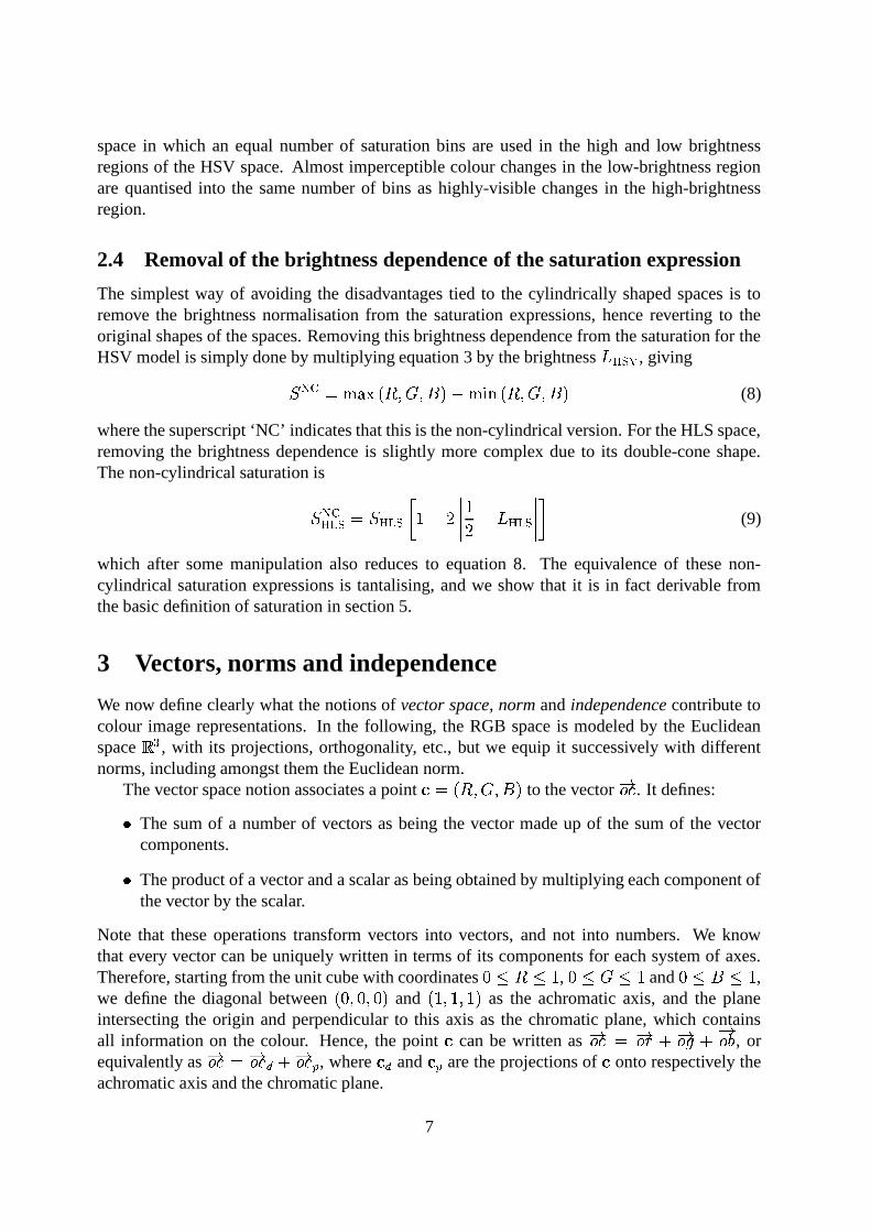
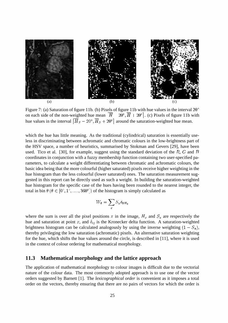
In practice, for images which contain only strongly saturated colours, there is not a signifi-cant difference between the values of weighted and unweighted hue means. Figure 11b showsan image in which this difference is important. As is visible in figure 7a, the saturation of the twobrown cells is higher than the saturation of the surroundings. For this image, the unweighted huemean is

4 4 � 8+;�7 �DC, and the saturation-weighted hue mean is

4 � 4 � ��7A@ C. To show the differ-

ence, thresholds on the hue band image were calculated for the intervals � 4 � 8+� C�� 4 = 8+� C and � 4 � � 8+� C � 4 � = 8+� C

, and these are shown in figures 7b and 7c respectively. On examin-ing these images, it is clear the the saturation-weighted hue mean corresponds to the hue of themost highly saturated regions, the two cells, whereas the unweighted hue mean is skewed bythe hues associated with the surrounding low-saturation regions.

11.2 Hue histograms

Hue histograms are often used as an image feature for retrieval of colour images from databases.In these histograms, one generally wishes to exclude achromatic and near-achromatic pixels, for

24

(a) (b) (c)

Figure 7: (a) Saturation of figure 11b. (b) Pixels of figure 11b with hue values in the interval �����on each side of the non-weighted hue mean � ������ �� � ����� ��� . (c) Pixels of figure 11b withhue values in the interval � �������� �� ��������� ��� around the saturation-weighted hue mean.

which the hue has little meaning. As the traditional (cylindrical) saturation is essentially use-less in discriminating between achromatic and chromatic colours in the low-brightness part ofthe HSV space, a number of heuristics, summarised by Stokman and Gevers [29], have beenused. Tico et al. [30], for example, suggest using the standard deviation of the � , � and �coordinates in conjunction with a fuzzy membership function containing two user-specified pa-rameters, to calculate a weight differentiating between chromatic and achromatic colours, thebasic idea being that the more colourful (higher saturated) pixels receive higher weighting in thehue histogram than the less colourful (lower saturated) ones. The saturation measurement sug-gested in this report can be directly used as such a weight. In building the saturation-weightedhue histogram for the specific case of the hues having been rounded to the nearest integer, thetotal in bin ����� �"!#� �$&%'��&(�(&(�*)�+ � ��,.- of the histogram is simply calculated as/1032547698 6;: 0=<?>where the sum is over all the pixel positions @ in the image, � 6 and

8 6are respectively the

hue and saturation at point @ , and

:�A#Bis the Kronecker delta function. A saturation-weighted

brightness histogram can be calculated analogously by using the inverse weighting � % � 8 6 - ,thereby privileging the low saturation (achromatic) pixels. An alternative saturation weightingfor the hue, which shifts the hue values around the circle, is described in [11], where it is usedin the context of colour ordering for mathematical morphology.

11.3 Mathematical morphology and the lattice approach

The application of mathematical morphology to colour images is difficult due to the vectorialnature of the colour data. The most commonly adopted approach is to use one of the vectororders suggested by Barnett [1]. The lexicographical order is convenient as it imposes a totalorder on the vectors, thereby ensuring that there are no pairs of vectors for which the order is

25

(a) (b)

(c)

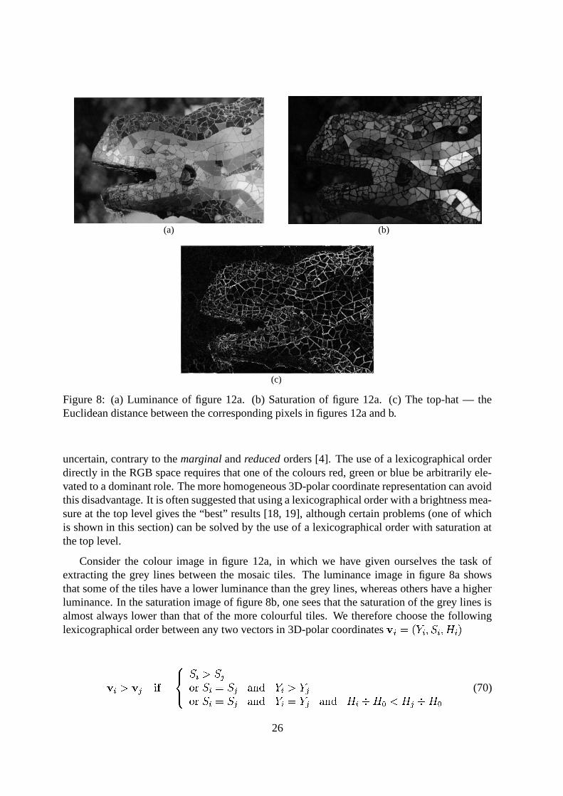
Figure 8: (a) Luminance of figure 12a. (b) Saturation of figure 12a. (c) The top-hat — theEuclidean distance between the corresponding pixels in figures 12a and b.

uncertain, contrary to the marginal and reduced orders [4]. The use of a lexicographical orderdirectly in the RGB space requires that one of the colours red, green or blue be arbitrarily ele-vated to a dominant role. The more homogeneous 3D-polar coordinate representation can avoidthis disadvantage. It is often suggested that using a lexicographical order with a brightness mea-sure at the top level gives the “best” results [18, 19], although certain problems (one of whichis shown in this section) can be solved by the use of a lexicographical order with saturation atthe top level.

Consider the colour image in figure 12a, in which we have given ourselves the task ofextracting the grey lines between the mosaic tiles. The luminance image in figure 8a showsthat some of the tiles have a lower luminance than the grey lines, whereas others have a higherluminance. In the saturation image of figure 8b, one sees that the saturation of the grey lines isalmost always lower than that of the more colourful tiles. We therefore choose the followinglexicographical order between any two vectors in 3D-polar coordinates ����� ��� ����� �������

��������� ������� ������� "! ����#��%$'&)( � �*� � � "! ����#��%$'&)( � �+� � �%$,&)( �-��.��0/213�4�5.6�0/ (70)

26

where the symbol � on the last level represents the acute angle between two angular values, i.e.

� � � ��� 4 � � � � � ����

,-, � � � � ����� �

��DC� ;<�DC � � � � � ���

�,-, � � � � ���

� �G���DC (71)

The variable4 �

on the third level of the lexicographical order is the position of the origin ofthe hue circle. As the third level of a lexicographical order is hardly ever used in practice [12],its value does not have much effect on the results. Applying a morphological closing using thisorder with a square structuring element of size

B � Bpixels to figure 12a produces figure 12b, in

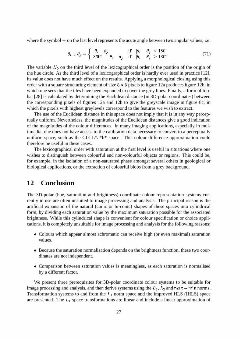
which one sees that the tiles have been expanded to cover the grey lines. Finally, a form of top-hat [28] is calculated by determining the Euclidean distance (in 3D-polar coordinates) betweenthe corresponding pixels of figures 12a and 12b to give the greyscale image in figure 8c, inwhich the pixels with highest greylevels correspond to the features we wish to extract.

The use of the Euclidean distance in this space does not imply that it is in any way percep-tually uniform. Nevertheless, the magnitudes of the Euclidean distances give a good indicationof the magnitudes of the colour differences. In many imaging applications, especially in mul-timedia, one does not have access to the calibration data necessary to convert to a perceptuallyuniform space, such as the CIE L*a*b* space. This colour difference approximation couldtherefore be useful in these cases.

The lexicographical order with saturation at the first level is useful in situations where onewishes to distinguish between colourful and non-colourful objects or regions. This could be,for example, in the isolation of a non-saturated phase amongst several others in geological orbiological applications, or the extraction of colourful blobs from a grey background.

12 Conclusion

The 3D-polar (hue, saturation and brightness) coordinate colour representation systems cur-rently in use are often unsuited to image processing and analysis. The principal reason is theartificial expansion of the natural (conic or bi-conic) shapes of these spaces into cylindricalform, by dividing each saturation value by the maximum saturation possible for the associatedbrightness. While this cylindrical shape is convenient for colour specification or choice appli-cations, it is completely unsuitable for image processing and analysis for the following reasons:� Colours which appear almost achromatic can receive high (or even maximal) saturation

values.� Because the saturation normalisation depends on the brightness function, these two coor-dinates are not independent.� Comparison between saturation values is meaningless, as each saturation is normalisedby a different factor.

We present three prerequisites for 3D-polar coordinate colour systems to be suitable forimage processing and analysis, and then derive systems using the

� �,� �

and #�� � J,./ norms.Transformation systems to and from the

���norm space and the improved HLS (IHLS) space

are presented. The���

space transformations are linear and include a linear approximation of

27

the hue. This space should therefore be used if very efficient transformations are required. TheIHLS space is more suited to image analysis tasks, as it permits a wide choice of brightnessfunctions and does not approximate the hue. Any 3D-polar coordinate system is very closelytied to the RGB space, being simply a different representation of it. It therefore does not haveany of the good properties of the L*a*b* or L*u*v* spaces, such as perceptual uniformity. Itsadvantages are that the conversion algorithm is very simple, and that no colour calibration data,such as the white point coordinates, are required. This calibration data is usually not availablein multimedia applications, for example.

Three applications demonstrating the good properties of the suggested saturation measureare given. The calculation of statistics of the hue weighted by the saturation and the determina-tion of the saturation-weighted hue histogram use the fact that the suggested saturation measureis always small for near-achromatic colours. The mathematical morphology application takesadvantage of the ability to do comparisons between the saturation values.

In summary, much confusion and incompatibility between results in colour image process-ing and analysis could be avoided by the use of the suggested 3D-polar coordinate system.

A Proof of the independence of the proposed saturation andthe brightness function

We give a proof of the independence of the brightness and saturation, stated in section 5. Con-sider the triangle shown in figure 5a, which contains all the points with the same hue as

1. This

triangle is reproduced in figure 9 to facilitate the following proof.

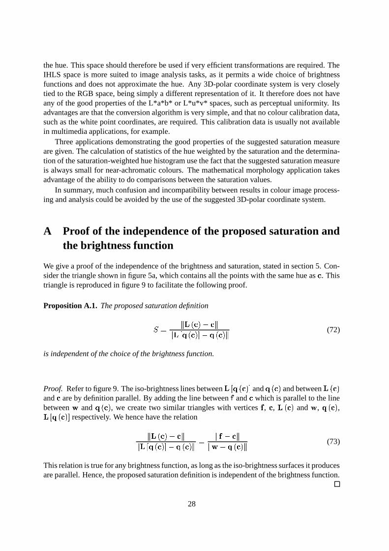
Proposition A.1. The proposed saturation definition

4 ����13 � 1��

��

���13 � � �

�213 � (72)

is independent of the choice of the brightness function.

Proof. Refer to figure 9. The iso-brightness lines between �

��213 �

and ���13

and between ��213

and1

are by definition parallel. By adding the line between � and1

which is parallel to the linebetween � and �

��13, we create two similar triangles with vertices � ,

1, �

��13and � , �

��13,

�

�� 13E�

respectively. We hence have the relation

����13 � 1��

��

��213 � � �

�213 � 4�

� � 1��� � � �

��13 � (73)

This relation is true for any brightness function, as long as the iso-brightness surfaces it producesare parallel. Hence, the proposed saturation definition is independent of the brightness function.

28

w= (1,1,1)

o = (0,0,0)

c

L c

q c

f

( )

( )

L q c[ ]( )

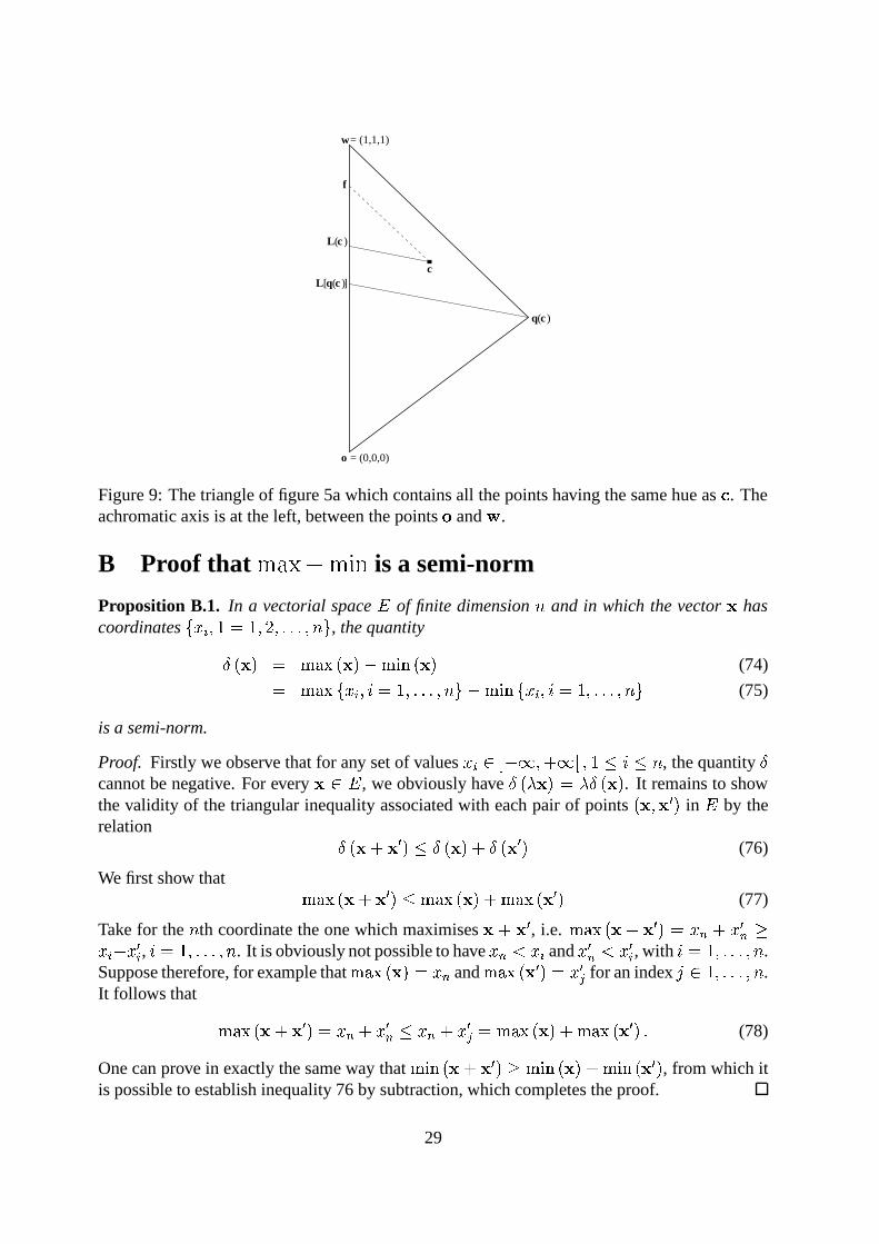
Figure 9: The triangle of figure 5a which contains all the points having the same hue as1. The

achromatic axis is at the left, between the points � and � .

B Proof that ������� ��� is a semi-norm

Proposition B.1. In a vectorial space � of finite dimension � and in which the vector � hascoordinates ��� � ��� 4 �<� 8���7�7�7�� � � , the quantity

�� � 4 #�� � � � , / � � (74)4 #�� ��� � � � 4 �<��7�7�7�� � � � J,./ ��� � ��� 4 �<��7�7�7�� � � (75)

is a semi-norm.

Proof. Firstly we observe that for any set of values � � � � ��� � = � ��� � � � � , the quantity �cannot be negative. For every � � � , we obviously have �

� � � 4 � �� � . It remains to show

the validity of the triangular inequality associated with each pair of points� � � � 5 in � by the

relation�� � = � 5 � �

� � = �� � 5 (76)

We first show that #.� � � = � 5 � #.� � � = #.� � � 5 (77)

Take for the � th coordinate the one which maximises � = � 5 , i.e. #.� � � = � 5 4 � � = � 5� �� � = � 5� , � 4 �+��7�7�7 � � . It is obviously not possible to have � � � � � and � 5� � � 5� , with

� 4 �<��7�7�7�� � .Suppose therefore, for example that #.� � � 54 � � and #.� � � 5 54 � 5� for an index � � �+��7�7�7 � � .It follows that

#�� � � = � 5 54 � � = � 5� ��� � = � 5� 4 #�� � � = #.� � � 5 7 (78)

One can prove in exactly the same way that J,./ � � = � 5 � J,./ � � = J,./ � � 5 , from which itis possible to establish inequality 76 by subtraction, which completes the proof.

29

Acknowledgments

Thank you to Jesus Angulo and Walter Kropatsch for their extremely useful comments on themanuscript.

References

[1] V. Barnett. The ordering of multivariate data. Journal of the Statistical Society of AmericaA, 139(3):318–354, 1976.

[2] Thierry Carron. Segmentations d’images couleur dans la base Teinte-Luminance-Saturation: approche numerique et symbolique. PhD thesis, Universite de Savoie, 1995.

[3] Vicent Caselles, Bartomeu Coll, and Jean-Michel Morel. Geometry and color in naturalimages. Journal of Mathematical Imaging and Vision, 16:89–105, 2002.

[4] Mary L. Comer and Edward J. Delp. Morphological operations for colour image process-ing. Journal of Electronic Imaging, 8(3):279–289, 1999.

[5] Commission Internationale de l’Eclairage. International Lighting Vocabulary. Number17.4. CIE, 4th edition, 1987.

[6] Claire-Helene Demarty. Segmentation et Structuration d’un Document Video pour la Car-acterisation et l’Indexation de son Contenu Semantique. PhD thesis, CMM, Ecole desMines de Paris, 2000.

[7] Claire-Helene Demarty and Serge Beucher. Color segmentation algorithm using an HLStransformation. In Proceedings of the International Symposium on Mathematical Mor-phology (ISMM ’98), pages 231–238, 1998.

[8] N. I. Fisher. Statistical Analysis of Circular Data. Cambridge University Press, 1993.

[9] T. Gevers and A. W. M. Smeulders. A comparative study of several color models for colorimage invariant retrieval. In Proceedings of the First International Workshop, IDB-MMS,pages 17–26, August 1996.

[10] Allan Hanbury. The taming of the hue, saturation and brightness colour space. In Pro-ceedings of the Seventh Computer Vision Winter Workshop, Bad Aussee, Austria, 2002.

[11] Allan Hanbury and Jean Serra. Mathematical morphology in the HLS colour space. In TimCootes and Chris Taylor, editors, Proceedings of the British Machine Vision Conference2001, pages 451–460. BMVA, 2001.

[12] Allan Hanbury and Jean Serra. Mathematical morphology in the L*a*b* colour space.Technical Report N-36/01/MM, CMM, Ecole des Mines de Paris, 2001.

[13] Allan Hanbury and Jean Serra. Morphological operators on the unit circle. IEEE Trans-actions on Image Processing, 10(12):1842–1850, December 2001.

30

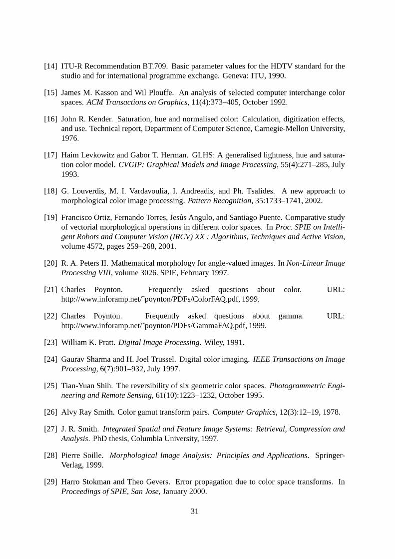
[14] ITU-R Recommendation BT.709. Basic parameter values for the HDTV standard for thestudio and for international programme exchange. Geneva: ITU, 1990.

[15] James M. Kasson and Wil Plouffe. An analysis of selected computer interchange colorspaces. ACM Transactions on Graphics, 11(4):373–405, October 1992.

[16] John R. Kender. Saturation, hue and normalised color: Calculation, digitization effects,and use. Technical report, Department of Computer Science, Carnegie-Mellon University,1976.

[17] Haim Levkowitz and Gabor T. Herman. GLHS: A generalised lightness, hue and satura-tion color model. CVGIP: Graphical Models and Image Processing, 55(4):271–285, July1993.

[18] G. Louverdis, M. I. Vardavoulia, I. Andreadis, and Ph. Tsalides. A new approach tomorphological color image processing. Pattern Recognition, 35:1733–1741, 2002.

[19] Francisco Ortiz, Fernando Torres, Jesus Angulo, and Santiago Puente. Comparative studyof vectorial morphological operations in different color spaces. In Proc. SPIE on Intelli-gent Robots and Computer Vision (IRCV) XX : Algorithms, Techniques and Active Vision,volume 4572, pages 259–268, 2001.

[20] R. A. Peters II. Mathematical morphology for angle-valued images. In Non-Linear ImageProcessing VIII, volume 3026. SPIE, February 1997.

[21] Charles Poynton. Frequently asked questions about color. URL:http://www.inforamp.net/˜poynton/PDFs/ColorFAQ.pdf, 1999.

[22] Charles Poynton. Frequently asked questions about gamma. URL:http://www.inforamp.net/˜poynton/PDFs/GammaFAQ.pdf, 1999.

[23] William K. Pratt. Digital Image Processing. Wiley, 1991.

[24] Gaurav Sharma and H. Joel Trussel. Digital color imaging. IEEE Transactions on ImageProcessing, 6(7):901–932, July 1997.

[25] Tian-Yuan Shih. The reversibility of six geometric color spaces. Photogrammetric Engi-neering and Remote Sensing, 61(10):1223–1232, October 1995.

[26] Alvy Ray Smith. Color gamut transform pairs. Computer Graphics, 12(3):12–19, 1978.

[27] J. R. Smith. Integrated Spatial and Feature Image Systems: Retrieval, Compression andAnalysis. PhD thesis, Columbia University, 1997.

[28] Pierre Soille. Morphological Image Analysis: Principles and Applications. Springer-Verlag, 1999.

[29] Harro Stokman and Theo Gevers. Error propagation due to color space transforms. InProceedings of SPIE, San Jose, January 2000.

31

[30] Marius Tico, Taneli Haverinen, and Pauli Kuosmanen. A method of color histogram cre-ation for image retrieval. In Proceedings of NORSIG, 2000.

32

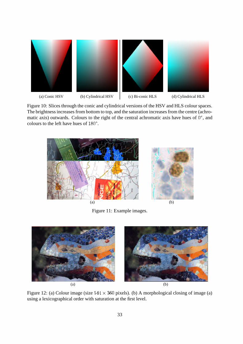
(a) Conic HSV (b) Cylindrical HSV (c) Bi-conic HLS (d) Cylindrical HLS

Figure 10: Slices through the conic and cylindrical versions of the HSV and HLS colour spaces.The brightness increases from bottom to top, and the saturation increases from the centre (achro-matic axis) outwards. Colours to the right of the central achromatic axis have hues of

� C, and

colours to the left have hues of�

�� C

.

(a) (b)

Figure 11: Example images.

(a) (b)

Figure 12: (a) Colour image (sizeB B B � � ;<�

pixels). (b) A morphological closing of image (a)using a lexicographical order with saturation at the first level.

33