a 30m sub/millimeter survey telescope to probe dusty, star

A 30m Sub/Millimeter Survey Telescope to Probe Dusty, Star-Forming Galaxies

into the Epoch of ReionizationThe Reionization Epoch:

New Insights and Future Prospects2016/03/08

S. Golwala (Caltech) for many others

A 30-m Sub/mm Survey Telescope to Probe DSFGs into the EoR 2016/03/08

What do dusty, star-forming galaxies have to do with reionization?

Reionization is a critical observable forconstraininggalaxy evolutionMust have enough

star formation toproduce ionizingphotons

Must not form starsso quickly that dusttoo quickly begins toabsorb UV photons

Tracing the rise of DSFGs is necessary topiece together the puzzle of how galaxies reionizedthe universe

2

4 Robertson et al.

Fig. 3.— Measures of the neutrality 1 − QHIIof the inter-

galactic medium as a function of redshift. Shown are the ob-servational constraints compiled by Robertson et al. (2013), up-dated to include recent IGM neutrality estimates from the ob-served fraction of Lyman-α emitting galaxies (Schenker et al. 2014;Pentericci et al. 2014), constraints from the Lyman-α of GRB hostgalaxies (Chornock et al. 2013), and inferences from dark pixels inLyman-α forest measurements (McGreer et al. 2015). The evolv-ing IGM neutral fraction computed by the model is also shown (redregion is the 68% credibility interval, white line is the ML model).While these data are not used to constrain the models, they arenonetheless remarkably consistent. The bottom panel shows theIGM neutral fraction near the end of the reionization epoch, wherethe presented model fails to capture the complexity of the reion-ization process. For reference we also show the corresponding in-ferences calculated from Robertson et al. (2013) (blue region) anda model forced to reproduce the WMAP τ (orange region).

Figure 3 also shows the earlier model ofRobertson et al. (2013) (blue region) which com-pletes reionization at slightly lower redshift and displaysa more prolonged ionization history. This model wasin some tension with the WMAP τ (Figure 2). If weforce the model in the present paper to reproduce theWMAP τ (orange region), reionization ends by z ∼ 7.5,which is quite inconsistent with several observationsthat indicate neutral gas within IGM over the range6 ! z ! 8 (Figure 3).

3. CONSTRAINTS ON THE CONTRIBUTION OF Z > 10GALAXIES TO EARLY REIONIZATION

By using the parameterized model of MD14 to fit thecosmic SFR histories, and applying a simple analyticalmodel of the reionization process, we have demonstratedthat SFR histories consistent with the observed ρSFR(z)integrated to Lmin = 0.001L⋆ reproduce the observedPlanck τ while simultaneously matching measures of theIGM neutral fraction at redshifts 6 ! z ! 8. As Fig-ure 1 makes apparent, the parameterized model extendsthe inferred SFR history to z > 10, beyond the reach

measurements when QHII∼ 1 because of our simplified treatment

of the ionization process (see the discussion in Robertson et al.2013)

Fig. 4.— Correspondence between the Thomson optical depth,the equivalent instantaneous reionization redshift zreion, and theaverage SFR density ρSFR at redshift z " 10. Shown are samples(points) from the likelihood function of the ρSFR model parametersresulting in the 68% credibility interval on τ from Figure 2, colorcoded by the value of zreion. The samples follow a tight, nearlylinear correlation (dashed line) between ρSFR and τ , demonstratingthat in this model the Thomson optical depth is a proxy for thehigh-redshift SFR. We also indicate the number of z > 10 galaxieswith mAB < 29.5 per arcmin−2 (right axis), assuming the LFshape does not evolve above z > 10.

of current observations. Correspondingly, these galaxiessupply a non-zero rate of ionizing photons that enable theThomson optical depth to slowly increase beyond z ∼ 10(see Figure 2). We can therefore ask whether a connec-tion exists between ρSFR(z > 10) and the observed valueof τ under the assumption that star forming galaxies con-trol the reionization process.Figure 4 shows samples from the likelihood function of

our model parameters given the ρSFR(z) and τ empiricalconstraints that indicate the mean SFR density ⟨ρSFR⟩(averaged over 10 ! z ! 15) as a function of the totalThomson optical depth τ . The properties ⟨ρSFR⟩ and τare tightly related, such that the linear fit

⟨ρSFR⟩ ≈ 0.344(τ − 0.06) + 0.00625 [M⊙ yr−1 Mpc−3](6)

provides a good description of their connection (dashedline). For reference, the likelihood samples shown in Fig-ure 4 indicate the corresponding redshift of instantaneousreionization zreion via a color coding.Given that the SFR density is supplied by galaxies that

are luminous in their rest-frame UV, we can also connectthe observed τ to the abundance of star forming galaxiesat z " 10. This quantity holds great interest for fu-ture studies with James Webb Space Telescope, as thepotential discovery and verification of distant galaxiesbeyond z > 10 has provided a prime motivation for theobservatory. The 5-σ sensitivity of JWST at 2 µm in at = 104 s exposure is mAB ≈ 29.5.7 At z ∼ 10, this

7 See http://www.stsci.edu/jwst/instruments/nircam/sensitivity/table

Robertson et al 2015DSFGs?


DSFGs dominate SFR density at epoch of peak SFR, z ~1-3L,IR ≈ 1012 LSun, SFR ~ 200 MSun/yrhyperlum. starbursts: > 2000 MSun/yr, 1013 LSun

How did they arise during EoR and afterward?

What is the history of DSFGs during and right after the epoch of reionization?

3

Cas

ey e

t al

201

4

86 C.M. Casey et al. / Physics Reports 541 (2014) 45–161

Fig. 22. The evolution of L? and ? for the integrated infrared luminosity function from the literature. One of two models is adopted in these works. LeFloc’h et al. (2005), Caputi et al. (2007) and Gruppioni et al. (2013) all use the model described in Eq. (14) while Goto et al. (2010), Magnelli et al. (2011)and Magnelli et al. (2013) use the model from Eq. (15). While L? shows clear signs of downsizing in all models, irrespective of absolute calibration, theevolution in ? is more model dependent.

Fig. 23. The contribution of various galaxy populations to the cosmic star formation rate density (left y-axis) or infrared luminosity density (right y-axis). The Kennicutt (1998a) scaling for LIR to SFR in Eq. (10) is assumed. This SFRD plot shows the contributions from total surveyed infrared populations,whereas Fig. 24 shows the break-down of contributions by luminosity bins between 0 < z < 2.5. All infrared-based estimates are compared to theoptical/rest-frame UV estimates compiled in Hopkins and Beacom (2006) which have been corrected for dust extinction, and therefore represent anapproximation to the total star formation rate density in the Universe at a given epoch. The total infrared estimates from the literature (integrated over108–1013.5L) come from Spitzer samples (Le Floc’h et al., 2005; Pérez-González et al., 2005; Caputi et al., 2007; Rodighiero et al., 2010; Magnelli et al.,2011) and Herschel samples (Gruppioni et al., 2013). In contrast, several samples from the submm and mm are also included; although they are knownto be incomplete, they provide a benchmark lower limits for the true contributions from their respective populations. These estimates include 850/870µm-selected SMGs (Chapman et al., 2005; Wardlow et al., 2011; Barger et al., 2012; Casey et al., 2013), 1.2 mm-selected MMGs (Roseboom et al., 2012),250–500 µm-selected Herschel DSFGs (Casey et al., 2012a,b) and 450 µm Scuba-2-selected DSFGs (Casey et al., 2013). See legend for color and symboldetails. (For interpretation of the references to color in this figure legend, the reader is referred to the web version of this article.)

measurement into redshift bins then gives more detailed information on sample evolution. Plots of SFRD against redshift orlook-back time are often referred to as a Lilly–Madau diagram, first discussed in Lilly et al. (1995) and Madau et al. (1996).

Fig. 23 illustrates infrared-based estimates to the SFRD contribution from a variety of surveys and Fig. 24 showstheir contributions broken down by luminosity class. Both of these SFRD figures provide essential illustrations to theinterpretation of cosmic star formation. While the first (Fig. 23) includes samples known to suffer from incompleteness andbiases, it is a useful tool for visualizing the net contribution from any one sample. For example, even though the 850 µm-selected SMG sample from Chapman et al. (2005) is known to be biased against warm-dust and radio-quiet galaxies, one can

86 C.M. Casey et al. / Physics Reports 541 (2014) 45–161

Fig. 22. The evolution of L? and ? for the integrated infrared luminosity function from the literature. One of two models is adopted in these works. LeFloc’h et al. (2005), Caputi et al. (2007) and Gruppioni et al. (2013) all use the model described in Eq. (14) while Goto et al. (2010), Magnelli et al. (2011)and Magnelli et al. (2013) use the model from Eq. (15). While L? shows clear signs of downsizing in all models, irrespective of absolute calibration, theevolution in ? is more model dependent.

Fig. 23. The contribution of various galaxy populations to the cosmic star formation rate density (left y-axis) or infrared luminosity density (right y-axis). The Kennicutt (1998a) scaling for LIR to SFR in Eq. (10) is assumed. This SFRD plot shows the contributions from total surveyed infrared populations,whereas Fig. 24 shows the break-down of contributions by luminosity bins between 0 < z < 2.5. All infrared-based estimates are compared to theoptical/rest-frame UV estimates compiled in Hopkins and Beacom (2006) which have been corrected for dust extinction, and therefore represent anapproximation to the total star formation rate density in the Universe at a given epoch. The total infrared estimates from the literature (integrated over108–1013.5L) come from Spitzer samples (Le Floc’h et al., 2005; Pérez-González et al., 2005; Caputi et al., 2007; Rodighiero et al., 2010; Magnelli et al.,2011) and Herschel samples (Gruppioni et al., 2013). In contrast, several samples from the submm and mm are also included; although they are knownto be incomplete, they provide a benchmark lower limits for the true contributions from their respective populations. These estimates include 850/870µm-selected SMGs (Chapman et al., 2005; Wardlow et al., 2011; Barger et al., 2012; Casey et al., 2013), 1.2 mm-selected MMGs (Roseboom et al., 2012),250–500 µm-selected Herschel DSFGs (Casey et al., 2012a,b) and 450 µm Scuba-2-selected DSFGs (Casey et al., 2013). See legend for color and symboldetails. (For interpretation of the references to color in this figure legend, the reader is referred to the web version of this article.)

measurement into redshift bins then gives more detailed information on sample evolution. Plots of SFRD against redshift orlook-back time are often referred to as a Lilly–Madau diagram, first discussed in Lilly et al. (1995) and Madau et al. (1996).

Fig. 23 illustrates infrared-based estimates to the SFRD contribution from a variety of surveys and Fig. 24 showstheir contributions broken down by luminosity class. Both of these SFRD figures provide essential illustrations to theinterpretation of cosmic star formation. While the first (Fig. 23) includes samples known to suffer from incompleteness andbiases, it is a useful tool for visualizing the net contribution from any one sample. For example, even though the 850 µm-selected SMG sample from Chapman et al. (2005) is known to be biased against warm-dust and radio-quiet galaxies, one can

Mad

au a

nd D

icki

nson

(20

14)?

reionization

A 30-m Sub/mm Survey Telescope to Probe DSFGs into the EoR 2016/03/08HFLS 3 is a massive, gas-rich galaxy. From the spectral energy distri-bution and the intensity of the CO and [C II] emission, we find a dustmass of Md 5 1.33 109 Msun and total molecular and atomic gas massesof respectively Mgas 5 1.0 3 1011 Msun and MHI 5 2.0 3 1010 Msun. Thesemasses are 15–20 times those of Arp 220, and correspond to a gas-to-dust ratio of ,80 and a gas depletion timescale of Mgas/SFR < 36 Myr.These values are comparable to lower-redshift submillimetre-selectedstarbursts11,12. From the [C I] luminosity, we find an atomic carbon massof 4.5 3 107 Msun. At the current SFR of HFLS 3, this level of carbonenrichment could have been achieved through supernovae on a timescaleof ,107 yr (ref. 13). The profiles of the molecular and atomic emissionlines typically show two velocity components (Fig. 1 and SupplementaryFigs 5 and 7). The gas is distributed over a region of 1.7 kpc radius with ahigh velocity gradient and dispersion (Fig. 3). This suggests a dispersion-dominated galaxy with a dynamical mass of Mdyn 5 2.7 3 1011 Msun. The

gas mass fraction in galaxies is a measure of the relative depletion andreplenishment of molecular gas, and is expected to be a function of halomass and redshift from simulations14. In HFLS 3, we find a high gas massfraction of fgas 5 Mgas/Mdyn < 40%, comparable to what is found in sub-millimetre-selected starbursts and massive star-forming galaxies at z < 2(refs 15, 16), but ,3 times higher than in nearby ultra-luminous infraredgalaxies (ULIRGs) like Arp 220, and .30 times higher than in the MilkyWay. From population synthesis modelling, we find a stellar mass ofM*5 3.7 3 1010 Msun, comparable to that of Arp 220 and about half thatof the Milky Way. This suggests that at most ,40% of Mdyn within theradius of the gas reservoir is due to dark matter. With up to ,1011 Msun ofdark matter within 3.4 kpc, HFLS 3 is likely to reside in a dark-matter halomassive enough to grow a present-day galaxy cluster17. The efficiencyof star formation is given by e 5 tdyn 3 SFR/Mgas, where tdyn 5 (r3/(2GM))1/2 is the dynamical (or free-fall) time, r is the source radius,

a

Arp 220 (z=0.0181)

CO

NH

[O I]

[N II]

H2O

Unlabelled lines, H2O

H2O

HFLS3 (z=6.3369)

5

10

15

20

25

0

30

Flux

den

sity

(mJy

)

600 800 1,000 1,200 1,400 1,600 1,800 2,000 2,200Qrest (GHz)

le f g h i j k onm

CO

COCO

CO NH3

[C II]

[C I]

OH

H2O+ H2O

H2O

OH+H2O

H2O

CO(J=6–5)

0.0

2.0

4.0

6.0

–4,00

0

–2,00

0 0

2,00

0

4,00

0

CO(J=2–1)

0.0

0.4

0.8

–4,00

0

–2,00

0 0

2,00

0

4,00

0

CO(J=3–2)

0.0

0.4

0.8

1.2

–2,00

0 0

2,00

0

4,00

0

6,00

0

CO(J=1–0)

–0.2

0.0

0.2

0.4

–2,00

0 0

2,00

0

H2O(211–202)

H2O+H2O

+

0.0

2.0

4.0

–5,00

0 0

5,00

0

CO(J=7–6) and [C I]

0.0

2.0

4.0

6.0

–4,00

0

–2,00

0 0

2,00

0

4,00

0

H2O(202–111)

2.0

4.0

6.0

–4,00

0

–2,00

0 0

2,00

0

CO(J=10–9)H2O(321–312)

5

10

15

–4,00

0

–2,00

0 0

2,00

0

CO(J=9–8)

OH+

2.0

4.0

6.0

8.0

–4,00

0

–2,00

0 0

2,00

0

H2O(312–303)

2.0

4.0

6.0

8.0

–2,00

0 0

2,00

0

4,00

0

OH+(112–012)

OH+

CO(J=9–8)

2.0

4.0

6.0

8.0

–4,00

0

–2,00

0 0

NH3(3,K)a–(2,K)sK=2,1,0

13

14

15

16

17

–2,00

0

–1,00

0 0

1,00

0

OH(2Π1/2 J=3/2–1/2)[–/+] [+/–]

CO

(J=1

6–15

)

15

20

25

–1,00

0 0

1,00

0

2,00

00

20

40

60

–1,00

0 0

1,00

0

2,00

0

CO

b d

CO

CO

150 200 300 350250

0.5

1.0

0.0

b c d e f g h

i j k l m n o[C II](2P3/2–2P1/2)

Velocity offset (km s–1)

c

Figure 1 | Redshift identification through molecular and atomicspectroscopy of HFLS 3. a, Black trace, wide-band spectroscopy in theobserved-frame 19–0.95-mm (histogram; rest-frame 2,600–130mm)wavelength range with CARMA (3 mm; ‘blind’ frequency scan of the full band),the PdBI (2 mm), the JVLA (19–6 mm) and CSO/Z-spec (1 mm; instantaneouscoverage). (CARMA, Combined Array for Research in Millimeter-waveAstronomy; PdBI, Plateau de Bure Interferometer; JVLA, Jansky Very LargeArray; and CSO, Caltech Submillimeter Observatory.) This uniquelydetermines the redshift of HFLS 3 to be z 5 6.3369 based on the detection of aseries of H2O, CO, OH, OH1, NH3, [C I] and [C II] emission and absorptionlines. b–o, Detailed profiles of detected lines (histograms; rest frequencies areindicated by corresponding letters in a). 1-mm lines (m–o) are deeper,interferometric confirmation observations for NH3, OH (both PdBI) and [C II]

(CARMA) not shown in a. The line profiles are typically asymmetric relative tosingle Gaussian fits, indicating the presence of two principal velocitycomponents at redshifts of 6.3335 and 6.3427. The implied CO, [C I] and [C II]line luminosities are respectively (5.08 6 0.45) 3 106 Lsun,(3.0 6 1.9) 3 108 Lsun and (1.55 6 0.32) 3 1010 Lsun. Strong rest-framesubmillimetre to FIR continuum emission is detected over virtually the entirewavelength range. For comparison, the Herschel/SPIRE spectrum of the nearbyultra-luminous infrared galaxy Arp 22020 is overplotted in grey (a). Lineslabelled in italic are tentative detections or upper limits (see SupplementaryTable 2). Most of the bright spectral features detected in Arp 22020,21 are alsodetected in HFLS 3 (in spectral regions not blocked by the terrestrialatmosphere). See Supplementary Information sections 2–4 for more details.

RESEARCH LETTER

3 3 0 | N A T U R E | V O L 4 9 6 | 1 8 A P R I L 2 0 1 3

Macmillan Publishers Limited. All rights reserved©2013

black/yellow: Herschel FLS-3 (z = 6.34)2900 MSun/yr, LIR = 4.2 x 1013 LSun

grey: Arp220 (z = 0.018)

How quickly do DSFGs arise in/after EoR?

Important test cases exist!HFLS-3: Extraordinary:

z ~ 6.3SFRIR ~2900 MSun/yrLIR ~ 4.2 x 1013 LSun Tdust = 56KSFRUV x103 smaller! Incredible

dust content at end of EoR

These objects crucial Show the outer limits

of what is possible at high z

Need to find many more to time birth of DSFGs, constrain rise of dust at z > 6Dimmer galaxies not visible to HerschelSED peak shifts to longer λ at higher z

Also: tracers of extreme overdensities at high z

4

M is the mass within radius r and G is the gravitational constant. Forr 5 1.7 kpc and M 5 Mgas, this suggests e 5 0.06, which is a few timeshigher than found in nearby starbursts and in giant molecular cloud coresin the Galaxy18.

The properties of atomic and molecular gas in HFLS 3 are fullyconsistent with a highly enriched, highly excited interstellar medium,

as typically found in the nuclei of warm, intense starbursts, but dis-tributed over a large, ,3.5-kpc-diameter, region. The observed COand [C II] luminosities suggest that dust is the primary coolant of thegas if both are thermally coupled. The L[CII]/LFIR ratio of ,5 3 1024 istypical for high radiation environments in extreme starbursts andactive galactic nucleus (AGN) host galaxies19. The L[CII]/LCO(1–0) ratioof ,3,000 suggests that the bulk of the line emission is associated withthe photon-dominated regions of a massive starburst. At the LFIR ofHFLS 3, this suggests an infrared radiation field strength and gasdensity comparable to nearby ULIRGs without luminous AGN(figures 4 and 5 of ref. 19).

From the spectral energy distribution of HFLS 3, we derive a dusttemperature of Tdust 5 56z9

12K, ,10 K less than in Arp 220, but ,3times that of the Milky Way. CO radiative transfer models assumingcollisional excitation suggest a gas kinetic temperature of Tkin 5144z59

30K and a gas density of log10(n(H2)) 5 3:80z0:280:17 cm-3 (Sup-

plementary Information section 4 and Supplementary Figs 13 and 14).These models suggest similar gas densities as in nearby ULIRGs, andprefer Tkin?Tdust, which may imply that the gas and dust are not inthermal equilibrium, and that the excitation of the molecular lines may bepartially supported by the underlying infrared radiation field. This isconsistent with the finding that we detect H2O and OH lines with upperlevel energies of E/kB . 300–450 K and critical densities of .108.5 cm23

at line intensities exceeding those of the CO lines. The intensities andratios of the detected H2O lines cannot be reproduced by radiative trans-fer models assuming collisional excitation, but are consistent with beingradiatively pumped by FIR photons, at levels comparable to thoseobserved in Arp 220 (Supplementary Figs 15 and 16)20,21. The CO andH2O excitation is inconsistent with what is observed in quasar hostgalaxies like Mrk 231 and APM 0827915255 at z 5 3.9, which lendssupport to the conclusion that the gas is excited by a mix of collisionsand infrared photons associated with a massive, intense starburst, ratherthan hard radiation associated with a luminous AGN22. The physical

10–1 100 101 102 103 104 105 106

λobs (μm)

10–5

10–4

10–3

10–2

10–1

100

101

102

Flux

(mJy

)

28

26

24

22

20

18

16

14

12

AB

mag

107 106 105 104 103 102 101

νrest (GHz)

MBBArp220M82HR10Eyelash

HFLS3

0 1 2 3 4 50

1

2

3

4

z=12

3

4

5

6

7

8

z=12

345 6 7 8

HFLS3 z=6.34

HLS A773 z=5.24

HATLAS ID141 z=4.24HFLS1 z=4.29

HFLS5 z=4.44

HLock102 z=5.29

S350μm > S250μm

S500μm > S350μm

Arp220M82

HR10Eyelash

250 μm 500 μm

1′

350 μm

S50

0μm

/ S

350μ

m

S350μm/S250μm

S500μm > 1.3 S350μm

a b

Figure 2 | Spectral energy distribution and Herschel/SPIRE colours ofHFLS 3. a, HFLS 3 was identified as a very high redshift candidate, as it appearsred between the Herschel/SPIRE 250-, 350- and 500-mm bands (inset). Thespectral energy distribution of the source (data points; lobs, observed-framewavelength; nrest, rest-frame frequency; AB mag, magnitudes in the AB system;error bars are 1s r.m.s. uncertainties in both panels) is fitted with a modifiedblack body (MBB; solid line) and spectral templates for the starburst galaxiesArp 220, M 82, HR 10 and the Eyelash (broken lines, see key). The implied FIRluminosity is 2:86z0:32

0:31 3 1013 Lsun. The dust in HFLS 3 is not optically thick atwavelengths longward of rest-frame 162.7mm (95.4% confidence;Supplementary Fig. 12). This is in contrast to Arp 220, in which the dustbecomes optically thick (that is, td 5 1) shortward of 234 6 3mm (ref. 20).Other high-redshift massive starburst galaxies (including the Eyelash) typicallybecome optically thick around ,200mm. This suggests that none of the

detected molecular/fine-structure emission lines in HFLS 3 require correctionfor extinction. The radio continuum luminosity of HFLS 3 is consistent with theradio–FIR correlation for nearby star-forming galaxies. b, Flux density ratios(350mm/250mm and 500mm/350mm) of HFLS 3. The coloured lines are thesame templates as in a, but redshifted between 1 , z , 8 (number labelsindicate redshifts). Dashed grey lines indicate the dividing lines for red(S250mm , S350mm , S500mm) and ultra-red (S250mm , S350mm and1.3 3 S350mm , S500mm) sources. Grey symbols show the positions of fivespectroscopically confirmed red sources at 4 , z , 5.5 (including three newsources from our study), which all fall outside the ultra-red cut-off. This showsthat ultra-red sources will lie at z . 6 for typical shapes of the spectral energydistribution (except those with low dust temperatures), whereas red sourcestypically are at z , 5.5. See Supplementary Information sections 1 and 3 formore details.

Table 1 | Observed and derived quantities for HFLS 3, Arp 220 andthe Milky Way

HFLS 3 Arp 220* Milky Way*

z 6.3369 0.0181Mgas (Msun) (1.04 6 0.09) 3 1011 5.2 3 109 2.5 3 109

Mdust (Msun) 1:31z0:320:30 3 109 ,1 3 108 ,6 3 107

M* (Msun)1 ,3.7 3 1010 ,(3–5) 3 1010 ,6.4 3 1010

Mdyn (Msun) || 2.7 3 1011 3.45 3 1010 2 3 1011 (,20 kpc)fgas (%)" 40 15 1.2LFIR (Lsun)# 2:86z0:32

0:31 3 1013 1.8 3 1012 1.1 3 1010

SFR (Msun yr21)q 2,900 ,180 1.3Tdust (K)** 55:9z9:3

12:066 ,19

For details see Supplementary Information section 3.*Literature values for Arp 220 and the Milky Way are adopted from refs 20 and 27–30. The totalmolecular gasmass of the Milky Way is uncertain by at least a factor of 2. Quoteddust massesand stellarmasses are typically uncertain by factors of 2–3 owing to systematics. The dynamical mass for the MilkyWay is quoted within the inner 20 kpc to be comparable to the other systems, not probing the outerregions dominated by dark matter. The dust temperature in the Milky Way varies by at least 65 Karound the quoted value, which is used as a representative value. Both Arp 220 and the Milky Way areknown to contain small fractions of significantly warmer dust. All errors are 1s r.m.s. uncertainties.Molecular gas mass, derived assuming aCO 5 Mgas/L9CO 5 1 Msun (K km s21 pc2)21 (seeSupplementary Information section 3.3).Dust mass, derived from spectral energy distribution fitting (see Supplementary Information section3.1).1 Stellar mass, derived from population synthesis fitting (see Supplementary Information section 3.4).||Dynamical mass (see Supplementary Information section 3.5)."Gas mass fraction, derived assuming fgas 5 Mgas/Mdyn (see Supplementary Information section 3.6).#FIR luminosity as determined over the range of 42.5–122.5mm from spectral energy distributionfitting (see Supplementary Information section 3.1).qSFR, derived assuming SFR (in Msun yr21) 5 1.0 3 10210 LFIR (in Lsun) (see SupplementaryInformation section 3.2).**Dust temperature, derived from spectral energy distribution fitting (see Supplementary Informationsection 3.1).

LETTER RESEARCH

1 8 A P R I L 2 0 1 3 | V O L 4 9 6 | N A T U R E | 3 3 1

Macmillan Publishers Limited. All rights reserved©2013

Riechers et al 2013

Riechers et al 2013


516 E. Bernhard et al.

Figure 4. UV luminosity function at z ∼ 5 and z ∼ 6 from LBG-selectedsamples. Black solid lines represent the UV luminosity function derivedfrom our best model. Red dotted lines represent the same model, but withoutscatter on the attenuation relation. Colored points are measurements fromvarious observational studies (Steidel et al. 1999; Bouwens et al. 2007).

3.4 Comparison with UV luminosity function of high-redshiftLBGs

We extended our model to z > 4 as a first-order test of whether thesimple ingredients we assumed at lower redshift are sufficient forreproducing high-redshift measurements as well. Unfortunately, wecurrently have no access to IR data at these redshifts, but UV lumi-nosity functions were measured using the Lyman-break-selectiontechnique (Steidel et al. 1996). However, our parametric massfunction based on Ilbert et al. (2013) was calibrated only up toz = 4. We thus used the fit of a compilation of mass function mea-surements coming from K-band-selected and Lyman break galaxies(LBG)-selected populations performed by Sargent et al. (in prepara-tion). Basic features of this compilation are a successive steepeningof the faint-end slope, a quickly declining characteristic density,and a decreasing M∗ with redshift. We assume no evolution of thesSFR–M and IRX–M relation beyond a redshift of 4 for the sake ofsimplicity.

Fig. 4 shows the comparison between our model (black solid line)and the data of Bouwens et al. (2007) and Steidel et al. (1999) atz ∼ 5 and 6. All the data points lie in the confidence area of ourempirical predictions (grey area). This demonstrates the predictive

power of our method and suggests that a non-evolving IRX–M andSFR–M relation at high-z is a fair hypothesis to interpret the currentdata. In a similar way as at lower redshifts, it is clear that a scatteron the attenuation relation is necessary to reproduce the bright-endof the UV luminosity functions at z ∼ 5 and 6.

4 IR PRO PERTIES O F U V SELECTEDP O P U L AT I O N

The IR properties of UV-selected population are not expected to besimilar to those of the full population. Our model is a useful tool tounderstand how this selection biases the obtained results. We nowdiscuss recent observational results obtained on these UV-selectedpopulations, and how they can be interpreted by our model.

4.1 Mean attenuation in UV-selected galaxies

Heinis et al. (2013) studied the mean IRX of UV-selected popu-lations, measured with a stacking analysis as a function of LUV atz ∼ 1.5. The results are compatible with a plateau at 10IRX = 6.9± 1.0 between 109.5 and 1011 L⊙ (see Fig. 5). The flat trend comefrom the mix of low- and high-mass galaxies in each UV bin, butis not trivial to understand, because of the rising IRX–M relation(Heinis et al. 2014). However, our best model also predicts a flattrend in this LUV range (blue solid line on Fig. 5). This result isessentially caused by the scatter on the attenuation relation, sincewe find a rising trend in the absence of dispersion (red dotted line onFig. 5). This is another indication for the importance of the scatterin order to be able to model simultaneously the statistical propertiesUV and IR populations. At fixed UV luminosity, there is thus a mixbetween galaxies with higher SFR (mass) and attenuation and otherswith lower SFR (mass) and attenuation. This picture is consistentwith the distribution in the IRX–M diagram of populations selectedby UV luminosity recovered from the simulation of (Heinis et al.2014). Nevertheless, there is a 2σ systematic discrepancy around1010 L⊙. We tried to modify the scatter and the IRX–M relation

Figure 5. Mean attenuation as a function of UV luminosity at z ∼ 1.5.The blue solid line is the prediction of our best model; the grey area isthe associated 1σ confidence region. The red dotted line stands for themodel without scatter in the IRX–M relation. Inverted triangles are fromthe stacking analysis of Heinis et al. (2013). The hatched region indicatesthe parameter space where no object was found by Buat et al. (2012) in a0.025 deg2 field (see the discussion Section 4.2).

MNRAS 442, 509–520 (2014)

at California Institute of Technology on October 17, 2014

http://mnras.oxfordjournals.org/

Dow

nloaded from

200

MSu

n/yr

Standard IRX-β relation implies less dust in rest-frame UV galaxies at z > 3.5

Known deviations from IRX-β relation at high LIR: UV and IR sightlines become mismatched

Maybe they are the same galaxies, with scatter in IRX from stochastic fluctuations in dust content into EoR (Bernhard et al 2014)?

Are they just different populations?

How do DSFGs connect to the galaxies that produce ionizing UV photons?

5

Bernhard et al 2014

?

[Gil de Paz et al (2007) and Howell et al (2010)]

Casey et al 2014Goldader et al 2002

log LUV [LSun]log LIR [LSun]9 10 11 12 13-2 0 2 4

𝞫

3

2

1

0

-1

-2

-3

∆𝞫 fr

om IR

X-𝞫

rel

atio

n

6

4

2

0

IRX

= lo

g 10(

L FIR

/LU

V)

-1 0 1 2 3

log SFR [MSun/yr]c.f. Reddy et al 2015 also

tail end of EoR

A Wide-Area Sub/Millimeter Imaging and Spectroscopy Survey/Golwala 2016/02/29

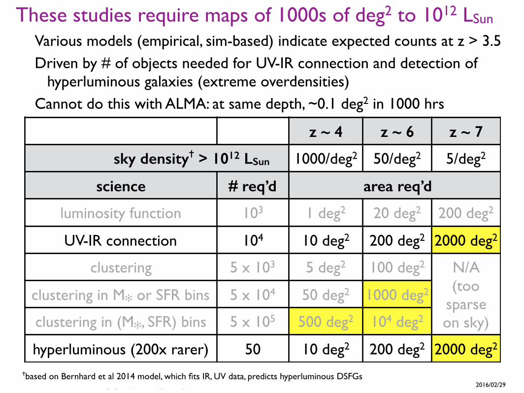
Various models (empirical, sim-based) indicate expected counts at z > 3.5Driven by # of objects needed for UV-IR connection and detection of

hyperluminous galaxies (extreme overdensities)Cannot do this with ALMA: at same depth, ~0.1 deg2 in 1000 hrs

These studies require maps of 1000s of deg2 to 1012 LSun

6

z ~ 4 z ~ 6 z ~ 7

sky density > 1012 LSun 1000/deg2 50/deg2 5/deg2

science # req’d area req’d

luminosity function 103 1 deg2 20 deg2 200 deg2

UV-IR connection 104 10 deg2 200 deg2 2000 deg2

clustering 5 x 103 5 deg2 100 deg2 N/A (too

sparse on sky)

clustering in M or SFR bins 5 x 104 50 deg2 1000 deg2

clustering in (M, SFR) bins 5 x 105 500 deg2 104 deg2

hyperluminous (200x rarer) 50 10 deg2 200 deg2 2000 deg2

based on Bernhard et al 2014 model, which fits IR, UV data, predicts hyperluminous DSFGs


Chajnantor Sub/millimeter Survey Telescope

Low-cost, 30m, 850µm 1° FoVLight, “minimal” mount

Primary floats on single-point support atcenter-of-gravity

Hexapod operates in balanced, “weightless” mode (except for wind & seismic): hexapod is repeatable

1 rad range-of-motion: 20,000 deg2 at equator1o diffraction-limited FoV at 850 µm

at single forward instrument mount

Cheap materials, sophisticated design and controlsMachined Al panels on steel truss

Simple mechanisms: No cable wrapsLight, exposed structureActive surface and offset guiding

corrects wind and thermal deformations7

Padin,Appl Opt (2014)


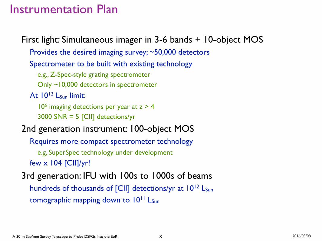
Instrumentation Plan

First light: Simultaneous imager in 3-6 bands + 10-object MOSProvides the desired imaging survey; ~50,000 detectors

Spectrometer to be built with existing technologye.g., Z-Spec-style grating spectrometerOnly ~10,000 detectors in spectrometer

At 1012 LSun limit:106 imaging detections per year at z > 43000 SNR = 5 [CII] detections/yr

2nd generation instrument: 100-object MOSRequires more compact spectrometer technology

e.g, SuperSpec technology under development

few x 104 [CII]/yr!

3rd generation: IFU with 100s to 1000s of beamshundreds of thousands of [CII] detections/yr at 1012 LSun

tomographic mapping down to 1011 LSun

8


CSST provides required survey speed for DSFG clustering measurements into EoR

CSST maps 1000 deg2/yr to 1012 L⊙ 1000 hrs/yr with 1° FoV and excellent site: meets requirement for clustering measurements.

~100x higher for 30m than existing, comparable resolution telescopes

9

Accounts for weather, opacityAssumes 100% survey operations

30m: 1000 deg2/yr

H-ATLAS 4° x 5°

Carpenter

Various models (empirical, sim-based) give consistent expectations for counts in z > 3.5 unexplored territory.


First-Light Spectroscopic Capabilities

10

Brad

ford

[O III] 88 µm (1.2 x 10-3)

[N II] 122 µm(3.1 x 10-4)

[N II] 205 µm(3.7 x 10-4) [O I] 145 µm

(1.1 x 10-4)

= 5σ detection

[C II] 158 µm (1.5 x 10-3)

Bright fine structure lines are shown,

with typical Lline/LIR

R = 1000 (300 km/s)

SNR = 5

30m


Comparison to ALMA

For a single object, ALMA ~10x more sensitive than 30mBoth ALMA receivers and 30m spectrometers are photon background limited

ALMA more sensitive due to enormous collecting area (10x)

10-object MOS matches ALMA for dust-obscured source z-searchThose without O/IR counterpart and thus no photo-zFor z-search, ALMA requires 8 tunings = x8 in time; 30m requires no such tunings.

10-12 beams makes up another factor of 10 in time

10-object MOS effective in identifying objects for critical ALMA followup1000 hrs/yr with 30m MOS (50% of available time) equivalent to 100 hrs/yr of ALMA

for sources with known z: 3000 [CII] SNR = 5 detections at 1012 LSun

use 30m [C II] to, e.g.:define samples with range of SF spatial extentsfind objects with anomalously low L[C II]/LFIR (small spatial extent)find objects with strong CH+

use ALMA followup tostudy [O I], [N II], [O III] to check [C II] calibration, measure effective stellar T in individual objectsstudy other tracers to measure morphology and kinematics of ionized and neutral gasmeasure neutral outflows precisely using wings of [C II] (and CO)

11


Complementarity with other facilities

LSST/Euclid/VISTA/WFIRSTCounterpart id to obtain photo-z

M, compl. SFR indicators (UV, Hα)Commensurate area

TMT, JWSTUV/O/IR spectroscopic followup:

HII region diagnosticsMorphology, comparison of UV to FIR

JVLA, SKACounterpart id

Radio SFR indicators (synchrotron, free-free)

ALMALower-level fine-structure linesMorphology and kinematics

Complementary area/depth surveys

FIR SurveyorIdeal for studying z < 3.5 populationUse dropouts to id z > 3.5 sources

12

10−3 10−2 10−1 100 101 102104

106

108

1010

1012

350µm850µm600MHz

S (mJy)

d3 N/d

S/dΩ

(gal

axie

s/Jy

/deg

2 )

Differential source counts vs. S

10−3 10−2 10−1 100 101 102100

102

104

106

350µm850µm600MHzo=Condon 1.4GHz

S (mJy)

N(>

S) (g

alax

ies/

deg2 )

Cumulative source counts vs. S

10−3 10−2 10−1 100 101 10210−2

100

102

104

30bps

30m 350µm30m 850µmSKA1 600MHz

vertical lines are ULIRG atz=2.5(7.5) solid(dashed)

S (mJy)

beam

s/so

urce

Confusion

10−3 10−2 10−1 100 101 10210−4

10−3

10−2

10−1

100

350µm850µm

S (mJy)

vertical lines are ULIRG atz=2.5(7.5) solid(dashed)SK

A so

urce

s in

a 30

m b

eam

Confusion

At depth sufficient to detect comparable objects(200 MSun/yr), <~1 src/30m 850 µm beam:

counterpart id should be unambiguous (even for O/IR-obscured objects)

Padi

n

600 MHz SKA

COSMOS 3.5 < z < 4.5

CSST 30 m

Vie

ira


Science Capabilities of CSST

Trace the evolution of dusty, star-forming galaxies (DSFGs) from z > 3.5 to z ≈ 1-3 when they dominate cosmic SFR by imaging 1000s of ° in multiple bands near 1 mm~ten DSFGs known at z > 3.5; largely unexplored territory. We’ll find >106 DSFGs/yr at z > 3.5!

Connection between dusty galaxies at z > 3.5 and rest-frame UV population: same or different?

Use DSFGs to identify extreme overdensities at high z

w/O/IR photo-z’s, use clustering to tie DSFGs to DM halos to track time evolution along main sequence

Measure molecular gas masses for z < 3.5 galaxies to provide gas mass, fraction, connection to SFR

Detail the drivers and impacts of star formation using spectroscopy of 1000s of galaxiesthe spatial extent of star formation

the physical conditions in the ionized and photodissociation regions around young stars

the characteristics of outflows and infall that are part of feedback loop that regulates SFR

Elucidate star formation locally by imaging nearby galaxies and large parts of our ownMap the fragmentation structure of molecular clouds and its connection to IMF

Study episodic accretion onto protostellar cores

Determine how rate and efficiency of star formation depend on M, environment, and galaxy morphology

Deepen our understanding of galaxy clusters and use them as cosmological tools via SZmeasure P, T, and v in the ICM to constrain the role of mergers, accretion, and energy injection

measure the cosmological peculiar velocity field to constrain cosmo params and deviations from GR

Find the unexpected!

14

a 30m sub/millimeter survey telescope to probe dusty, star

Documents