RESERVOIR ISSUE 03 • MARCH 2014 19

Register before April 11 at www.apegasummit.ca Info: 780-426-3990 | 800-661-7020 | #apegasummit

INTRODUCTIONIn some unconventional reservoirs, the presence of kerogen confounds standard log analysis models. Kerogen looks a lot like porosity to most porosity-indicating logs. Thus a single log, or any combination of them, will give highly optimistic porosity and free-gas or oil saturations, unless a kerogen correction is applied. This tutorial explains how such corrections can be applied in an otherwise standard petrophysical model that can be coded into the user-defined equation module of any software package.

Some quick-look methods “fake” the kerogen correction by using the density log with false and fixed matrix and/or fluid properties in an attempt to match core porosity (where it exists). When mineralogy varies, as in many unconventional reservoirs, the individual porosities calculated at each depth level are wrong, even though the average porosity may be correct. Porosity in the more dolomitic intervals will be too low and those in the higher quartz intervals will be too high. This will not help you decide where to position a horizontal well or help to assess net pay intervals because the porosity profile is extremely misleading.

Over-simplified techniques are dangerous, unprofessional, and unnecessary. Drawing an arbitrary straight line on a density log won’t “hack-it” in a world where wells cost multiple millions and a company’s stock price depends on the accuracy of the numbers in quarterly reports.

The 12-Step deterministic solution described here is easy to understand, easy to apply, and reasonably rapid. It is easier to manage than multi-mineral / statistical / probabilistic models. Parameter changes in later steps of the workflow will not change prior results, as happens in the multi-min environment. Each step in the model can be calibrated directly to available data before moving on to the next step. The workflow is simple, straight-forward, logical, controllable, and above all, predictable. BASIS FOR THE MODELThe methodology outlined below makes

use of well-known algorithms, run in a deterministic model that can be calibrated with available ground truth at every step of the process. Because of the sparse nature of some of the calibration data, it may have to come from offset wells, which forces us to analyze those wells in addition to the wells of primary interest. This extra work can be minimized when the proper data collection and lab work is planned as part of the initial drilling program.

One of the most widely used petrophysical porosity models in conventional reservoirs is the shale-corrected density-neutron complex lithology crossplot. It handles varying mineralogy and light hydrocarbon effects quite well and can use sonic data if the density goes AWOL in bad hole conditions. By extending the model to include a kerogen correction to each of the density, neutron, and sonic curves, we have a universal model that has proven effective over a wide range of unconventional reservoirs around the world. The model reverts to the standard model when kerogen volume is zero.

Other steps in the workflow use existing standard methods chosen because they work well in low porosity environments. There are many alternate models for every step and you may have a personal preference different than ours. Be sure to run a sensitivity test to confirm that the results are reasonable at low porosities with high clay volumes.

THE 12-STEP WORKFLOWThe petrophysical model for correcting porosity for kerogen involves calculation of kerogen weight and volume from suitable petrophysical models, and the modification of a few equations in the standard shale corrected density-neutron porosity model.

Step 1: Shale VolumeShale (or clay) volume is the most important starting point. Since many unconventional reservoirs are radioactive due to uranium associated with kerogen or phosphates, the usual clay volume model that depends on the gamma ray log needs special attention. Calibration to X-ray diffraction data (see example in Figure 1), or thin section point counts, is essential. The basic mineral mix also is developed from the XRD data set.

Shale volume calculations from a uranium corrected gamma ray curve (CGR) is the best bet:

1: VSHcgr = (CGR - CGR0) / (CGR100 - CGR0)

When CGR is not available, we fall back to the thorium (TH) curve from a spectral gamma ray log:

2: VSHth = (TH - TH0) / (TH100 - TH0)

When CGR and TH are missing, the total gamma ray curve (GR) can still be used by

A 12-STEP PROGRAM TO REDUCE UNCERTAINTY IN KEROGEN-RICH RESERVOIRS:Part 1 – Getting the Right Porosity| By E. R. (Ross) Crain, P.Eng., Spectrum 2000 Mindware Ltd., and Dorian Holgate, P.Geol., Aptian Technical Ltd.

Figure 1: Typical XRD analysis of a silty gas shale showing clay-quartz ratio averages of about 40:60% by weight. This would not be obvious from the gamma ray log due to uranium associated with the kerogen and/or phosphate minerals. Some radioactive reservoirs have nearly zero clay, so the XRD bulk clay volume is the best starting point for a petrophysical analysis

(Continued on page 20...)

20 RESERVOIR ISSUE 03 • MARCH 2014

moving the clean (GR0) and shale (GR100) lines further to the right compared to conventional shaly sands:

3: VSHgr = (GR - GR0) / (GR100 - GR0)

This last equation may take a little skill and daring, but that is what the XRD clay volumes are for. You can also test your clean and shale line picks in wells with CGR or TH curves then move that knowledge into other wells.

Unless shale volume is reasonably calibrated, nothing else in this workflow will work properly. Step 2: Kerogen Weight FractionKerogen weight fraction can be calculated from the resistivity log and a porosity log, using Passey or Issler methods. The Passey model is often called the “DlogR” method, with the “D” standing for “Delta-T” or sonic travel time. He also published density and neutron log versions of the equations. We have changed the abbreviations to reflect the three possible combinations:

4: SlogR = log (RESD / RESDbase) + 0.02 * (DTC – DTCbase)

5: Wtoc = SF1s * (SlogR * 10^(0.297 – 0.1688 * LOM)) + SO1s

OR

6: DlogR = log (RESD / RESDbase) – 2.5 * (DENS – DENSbase)

7: Wtoc = SF1d * (DlogR * 10^(0.297 – 0.1688 * LOM)) + SO1d OR

8: NlogR = log (RESD / RESDbase) -+ 4.0 * (PHIN – PHINbase)

9: Wtoc = SF1n * NDlogR * 10^(0.297 – 0.1688 * LOM)) + SO1n

Where: • XXXXbase = baseline log reading in non-

source rock shale• SlogR or DlogR or NlogR = Passey’s number

from sonic or density or neutron log (fractional)

• LOM = level of organic maturity (unitless)• Wtoc = total organic carbon from Passey

method (weight fraction)• SF1s,d,n and SO1s,d,n = scale factor and scale

offset to calibrate to lab values of TOC

The constants in the Passey equations require DTC values in usec/ft and density in g/cc.

The baseline values are supposed to be picked in non-source rock shales in the same geologic age as the reservoir, but there may be none in the area of interest. This makes the Passey model difficult to calibrate, hence the scale factor SF1 and scale offset SO1. LOM is seldom measured except as vitrinite reflectance (Ro). There is a published chart for converting Ro to LOM. LOM is in the range of 6 to 11 in gas shale and 11 to 18 in oil shale.

Issler’s method, which is based on WCSB Cretaceous data is preferred as no baselines are needed. It still needs a scale factor for deeper rocks. Tristan Euzen’s multiple regressions of the Issler graphs give:

10: TOCs = 0.0714 * (DTC + 195 * log(RESD)) - 31.86

11: Wtoc = SF2d * TOCs / 100 + SO2d OR 12: TOCd = -0.1429 * (DENS – 1014) /

(log(RESD) + 4.122) + 45.14

13: Wtoc = SF2s * TOCd / 100 + SO2s

Where: • Wtoc = total organic carbon from Issler

method (weight fraction)• SF2s,d and SO2s,d = scale factor and scale

offset to calibrate to lab values of TOC

The Issler equations expect density in Kg/m3 and sonic data in usec/m.

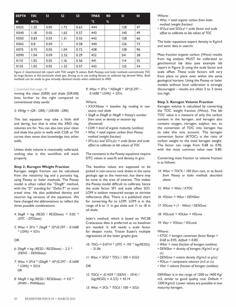
Mass fraction organic carbon (Wtoc) results from log analysis MUST be calibrated to geochemical lab data (see example lab report in Figure 2) using the scale factor and scale offset. These scale factors will vary from place to place even within the same geological horizon. Using the Passey or Issler models without local calibration is strongly discouraged – results are often 2 to 3 times too high.

Step 3: Kerogen Volume FractionKerogen volume is calculated by converting the TOC weight fraction (Wtoc). The lab TOC value is a measure of only the carbon content in the kerogen, and kerogen also contains oxygen, nitrogen, sulphur, etc, so the conversion of TOC into kerogen has to take this into account. The kerogen conversion factor (KTOC) is the ratio of carbon weight to the total kerogen weight. The factor can range from 0.68 to 0.95, with the most common value near 0.80. Converting mass fraction to volume fraction is as follows:

14: Wtoc = TOC% / 100 from core, or as found from Passey or Issler methods described above.

15: Wker = Wtoc / KTOC

16: VOLker = Wker / DENSker

17: VOLma = (1 - Wker) / DENSma

18: VOLrock = VOLker + VOLma

19: Vker = VOLker / VOLrock Where:• KTOC = kerogen conversion factor Range =

0.68 to 0.95, default = 0.80• Wker = mass fraction of kerogen (unitless)• DENSker = density of kerogen (Kg/m3 or g/

cc)• DENSma = matrix density (Kg/m3 or g/cc)• VOLxx = component volumes (m3 or cc)• Vker = volume fraction of kerogen (unitless)

DENSker is in the range of 1200 to 1400 Kg/m3, similar to good quality coal. Default = 1300 Kg/m3. Lower values are possible in low maturity kerogen.

DEPTH TOC S1 S2 S3 TMAX RO SI OI

M WT% °C %

X025 1.35 0.05 1.72 0.63 444 128 47

X040 1.18 0.05 1.65 0.57 443 140 49

X050 0.83 0.03 1.31 0.55 443 158 66

X065 0.8 0.04 1 0.58 440 126 73

X075 0.75 0.05 1.04 0.72 438 138 96

X090 1.04 0.09 2.52 0.29 452 241 28

X110 1.02 0.05 1.16 0.56 441 114 55

X135 1.05 0.05 1.32 0.57 443 125 54

Figure 2: Geochemical lab report with TOC weight % values. Both Passeyy and Issler methods overestimate TOC by large factors in this particular shale gas, forcing us to use scaling factors to calibrate log derived Wtoc. Both methods can be made to give virtually identical results when calibrated to XRD.

(...Continued from page 19)

RESERVOIR ISSUE 03 • MARCH 2014 21

Step 4: Kerogen and Shale Corrected PorosityEffective porosity is best calculated with the shale corrected density neutron complex lithology model, modified to correct for kerogen volume:

21: PHIDker = (2650 – DENSker) / 1650 (if PHIN is in Sandstone Units)

22: PHIdc = PHID – (Vsh * PHIDsh) – (Vker * PHIDker)

23: PHInc = PHIN – (Vsh * PHINsh) – (Vker * PHINker)

24: PHIe = (PHInc + PHIdc) / 2 PHINker is in the range of 0.45 to 0.75, similar to poor quality coal. Default = 0.65.

This model compensates for variations in mineralogy AND kerogen.

If the density log is affected by rough borehole, the shale corrected sonic log porosity (PHIsc) can be used instead:

24: PHISker = (DTCker – 182) / 474 (if PHIN is in Sandstone Units)

25: PHIsc = PHIS – (Vsh * PHISsh) – (Vker * PHISker)

26: PHInc = PHIN – (Vsh * PHINsh) – (Vker * PHINker)

27: PHIe = (PHInc + PHIsc) / 2

DTCker is in the range of 345 to 525 usec/m, similar to good quality coal. Default = 425 usec/m.

This model is moderately insensitive to variations in mineralogy AND compensates for kerogen.

Effective porosity from a nuclear magnetic resonance (NMR) log does not include kerogen or clay bound water, so this curve, where available, is a good test of the modified density neutron crossplot method shown above (illustrated in Figure 3). In all cases, good core control is essential. If porosity is too low compared to core porosity, then shale volume or kerogen volume are too high. Revisit the calibration of these two terms.

Some so-called shale gas zones are really tight gas with little kerogen or adsorbed gas, so the kerogen corrected complex lithology model

Figure 3: Example of TOC weight fraction (left hand curve in Track 1) calibrated to geochemical lab data in the Montney (2 dots near bottom of log segment – another 20+ data points are not shown to conserve space). Kerogen volume derived from TOC is displayed as dark shading to the left of effective porosity (shaded red) in Track 1. In the Doig above the Montney, there is no geochem data, so the NMR effective porosity (light grey curve) was used to back-calculate the TOC, based on the difference between raw neutron-density porosity and PHIEnmr values. Scale factors for the Doig and Montney are markedly different regardless of the TOC calculation method employed. Depth grid lines are 1 meter apart.(Continued on page 23...)

RESERVOIR ISSUE 03 • MARCH 2014 23

works well because it reverts to our standard methods automatically when Vker = 0.

CONCLUSIONS – PART 1A full suite of TOC and XRD mineralogy from samples, along with core porosity and saturation data, are needed to calibrate results from any petrophysical analysis of unconventional reservoirs. Bulk clay and TOC are the two critical lab measurements required through the interval of interest. Without valid calibration data, petrophysical analysis will have possible-error bars too large to allow meaningful financial decisions.

Of particular importance is the fact that Passey and Issler methods for determining TOC from logs will probably require a scale factor to match lab measured data. This fact is not well known and ignoring the problem can lead to large errors in porosity, free gas, and adsorbed gas estimations.

Part 2 of this article will describe the balance of the 12 Step Program for evaluating unconventional oil and gas reservoirs.

ABOUT THE AUTHORSE. R. (Ross) Crain, P.Eng. is a Consulting Petrophysicist and Professional Engineer, with over

50 years of experience in reservoir description, petrophysical analysis, and management. He is a specialist in the integration of well log analysis and petrophysics with geophysical, geological, engineering, stimulation, and simulation phases of the oil and gas industry, with widespread Canadian and Overseas experience. He has authored more than 60 articles and technical papers. His online shareware textbook, Crain’s Petrophysical Handbook, is widely used as a reference for practical petrophysical analysis methods. Mr. Crain is an Honourary Member and Past President of the Canadian Well Logging Society (CWLS), a Member of SPWLA, and a Registered Professional Engineer with APEGA ross@spec2000.net

Dorian Holgate is the principal consultant of Aptian

Technical Limited, an independent petrophysical consulting practice. He graduated from the University of Calgary with a B.Sc. in Geology in 2000 and completed the Applied Geostatistics Citation program from the University of Alberta in 2007. After graduation, he began working in the field for BJ Services (now Baker Hughes) and completed BJ’s Associate Engineer Program. Later, he joined BJ’s Reservoir Services Group, applying the analysis of well logs to rock mechanics to optimize hydraulic fracturing programs. In 2005, Dorian joined Husky Energy as a Petrophysicist and progressed to an Area Geologist role. He completed a number of petrophysical studies and built 3-D geological models for carbonate and clastic reservoirs. Dorian holds membership in APEGA, CSPG, SPE, SPWLA, and CWLS. dorian@aptianpetrophysics.com

(...Continued from page 21)

((((

((((

((((

((((

((((

((((

((((

((

((

((

((

((

((

((

((

((((

((((

((((

((((

((((

((((

((((

((((

((((

((((

((((

((((

((((

((((

((((

((((

((((

((((

((((

((((

((((

((((

((((

((((

((((

((((

((((

((

((

((((

((((

((((

((((

((((

((((

((((

((((

((((

((((

((((

((((

((((

((

((

((

((

((

((

((

((

((

((

((

((

((

((

((

((

((

((

((

((

((

((

((

((

((

((

((

((((

((((

((((

((((

((((((((

((((

((

((

((

((

((

((

((

((

((

((

((

((

((

((

((((

((((

((

((

((

((((

((

((

((

((((

((

((

((

((

((

((

((

((

((

((

((

((

((

((

((

((

((

((

((

((

((

((

((

((

((

((

((

((((

((

((

((

((((

((((

((((

((((

((((

((((

((((

((((

((((

((((

((((

((((

((((

((((

((((

((((

((((

((((

((((

((((

((((

((((

((((

((((

((((

((((

((((

((((

((((

((((

((((

((((

((((

((((

((((

((((

((((

((((

((((

((((

((((

((((

((((

((((

((((

((((

((((

((((

((((

((((

((((

((((

((((

((((

((((

((((

((((

((((

((((

((

((

((((

((((

((

((

((

((

((

((

((

((

((((

((((

((((

((((

((((

((

((

((

((

((

((

((

((

((

((

((

((

((

((

((

((

((

((((

((((

((((

((((

((

((

((

((((

((((

((

((

((((

((((

((((

((((

((((

((((

((((

((((

!!

!

!

!

!

!

!

!

!

!

!

!

!

!

!!

!

!

!

!

!!

!

!!

!

!

!

!

!

!

!

!

!

!

!

!!!

!!

")

")

")

")

")")

")

")

")")

")

")

")")

")

")")

")

")")

")

")")")

")

")

")")

")")

")

")

")")

")

")")

")

")

")

")")")

")")

")

")

")

")

")

")

")

")

")")")

")

")

")")

")")

")")

")

")")

")")

")

")

")

")

")

")

")

")

")

")

")

")

")

")

")

")")

")

")")

")

")")")

")

")")

")

")

")

")

")

")

")")")")

")

")

")")

")") ")

")")

")")

")

")")

")")")")

")

")")

")

")")

")

")")

")")

")

")")

")")

")

")")

")

")

")

")")

")

")

")

")

")

")

!

!

!

!

!

!

!

!

!

!

!

!

!!

! !

!

!

!

!!

!!!!

!!

!

!

30

40

35

35

35

40

35

3030

35

30

35

35

35

35

35

30

40

35

35

30

35

35

35

30

35

30

40

35

30

35

35

35

30

30

35

30

35

35

30

35

35

35

35

30

30

30

35

25

35

35

30

30

35

35

35

35

35

25

35

35

35

40

30

40

30

40

30

40

35

30

35

35

35

35

30

30

30

40

30

35

30

35

35

35

30

30

40

30

30

35

30

35

35

30

35

35

35

35

35

35

30

35

35

30

30

40

30

35

25

35

30

30

40

35

30

30

30

35

40

40

35

30

30

30

35

25

35

35

35

35

30

30

35

40

30

30

35

35

40

40

25

30

40

30

35

35

35

35

35

30

30

35

30

30

30

35

30

40

35

35

30

35

35

30

35

30

35

30

30

35

25

30

35

35

40

35

35

35

35

30

35

35

35

35

30

30

35

35

30

25

35

30

35

25

30

30

30

35

35

25

35

30

35

35

40

35

30

40

30

40

40

30

35

35

40

30

35

35

40

30

40

30

35

40

25

30

40

35

35

35

35

35

30

30

35

30

25

30

30

30

35

30

30

30

30

30

35

30

30

35

35

35

35

30

30

30

30

35

30

35

35

516

75

53

190118

45

10

82105

4274

30

4881

7592

142390

224101

109

142202200

300

143289

155120

AlbertaBritish Columbia Saskatchewan

Manitoba

Projection: UTM; Central Meridian -115.5; North American Datum 1983

1:600,000

0 10 20 30 40Km

Wells

! Duvernay Producers

! Gas Condensate Ratio

") Duvernay Cores (Preliminary)

") Duvernay Geochemistry Data (GSC, AGS)

Duvernay / Muskwa Isotherms (°C)60

80

100

120

Geothermal Gradient (All Units) °/1000mCI = 5 °C/1000m

High : 59

Low : 21

Structural and Geological Edges(( (( Paleozoic Deformation Front

Leduc Reefs (WCSB Atlas, 1994)

DuvernayGeothermal Gradient (All Units)

Copyright © 2013 Canadian Discovery Ltd. All Rights Reserved.

Author: M Fockler

Cartographer: C Keeler 1

Enclosure

Reviewer:

Filename: DVRN_GEOTHERMAL_ALL_MAP_PRELIM.mxd

Project: DVRN

Created: 21-January-2013

Last Edited: 16-July-2013

DVRN

T30

T45

T60

T65

T70

T75

T80R10

R20 R15 R10 R5 R1W5 R25R15

T50

T40

T30

T35

R5 R1W6 R25R20

R10W4

T80

T75

T70

T65

T60

T55

T45

R10W4R15R20R25R1W5R5R10R15

T35

T50

T55

West Shale Basin

East Shale Basin

Kaybob

T40

Edson

Karr

WillesdenGreen

((((

((((

((((

((((

((((

((((

((((

((((

((((

((((

((((

((

((((

((

((((

((((

((((

((((

((((

((((

((((

((((

((((

((((

((((

((((

((((

((((

((((

((((

((((

((

((((

((((

((((

((((

124697.23 miles322965.63 km

2

2

British ColumbiaManitoba

Alberta

SaskatchewanSaSkatchewan

alberta

britiSh columbia

the Duvernay ProjectWork on Canadian Discovery and partners’ Duvernay Project is well underway. This study evaluates the Geomechanics, Hydrocarbon Systems and Geological Setting of the Devonian Duvernay Formation in the Kaybob to Willesden Green Area.

TRICAN GEOLOGICAL SOLUTIONS

CanadianDiscoveryLtd.

GRAHAM DAVIES

CONSULTANTS LTD.

GEOLOGICAL

GDGC

Subscribe now and qualify for pre-completion pricing

Contact Cheryl Wrightcwright@canadiandiscovery.com | 403.269.3644

Image Left: Geothermal Gradient (All Units)

Results to date indicate:

» Variable lithology and a well-defined facies/lithology dependent fracture fabric

» Stratigraphy shows a possible extension to the current play areas

» Geochemistry shows source rock maturity is strongly related to heat flow variations

A geomechanical evaluation, detailed geochemistry, hydrogeology and reservoir mapping will be completed prior to study delivery.