9780203502815%2ech3

Chapter 3

COMPOSITE LAMINATES

3.1 Macromechanical behavior of lamina

In this chapter, we discuss some fundamental problems concerning fiber-reinforced composite laminates; i.e. the classical part of the general theory ofcomposite materials.

The basic results existing in this field can be found, for instance, in themonographies due to Ashton and Whitney [3.1], Jones [3.2], Christensen [3.3],Tsai and Hahn [3.4], Cristescu [3.5], Whitney [3.6] and Gibson [3.7].

The fiber-reinforced composite laminates are made of fiber-reinforced lam-inae. The fibers considered here are long and continuous. A lamina is a planearrangement of unidirectional fibers strongly bounded in a matrix. In Figure 3.1is shown a typical lamina together with its material symmetry axis, named alsoprincipal material axes or directions.

Figure 3.1: Lamina with unidirectional fibers.

Copyright © 2004 by Chapman & Hall/CRC

112 CHAPTER 3. COMPOSITE LAMINATES

Axis 1 is parallel to the fibers, axis 2 is perpendicular to the fibers in theplane of the lamina and axis 3 is perpendicular to the plane of lamina. The fibersor filaments are the main reinforcing or load-carrying elements. They are generallystrong and stiff. The matrix can be organic, ceramic, or metallic. The function ofthe matrix is to support and protect fibers and to provide a means of distributingand transmitting load among fibers. The fibers generally exhibit linear elasticbehavior. Fiber-reinforced composites, such as boron-epoxy and graphite-epoxy areusually considered to be linear elastic materials since the fibers provide most ofthe stiffness.

A laminate is a stack of laminae with various orientations of the principalmaterial directions with respect to the laminae as shown in Figure 3.2.

Figure 3.2: Exploded view of laminate structure.

Generally the fiber orientation of the layers cannot be symmetric about themiddle surface of the laminate. The layers of a laminate are usually firmly boundedtogether by the same matrix material that is used in laminae. Laminates can becomposed of plates of different materials, or layers of fiber-reinforced laminae, asshown in Figure 3.2. Also, various laminae can have various thicknesses.

A major purpose of lamination is to determine the directional dependenceof stiffness of a material in accordance with the given loading environment of thestructural element. Laminates are suited to this objective since the principal mate-rial directions of each layer can be oriented according to the need. For example, sixlayers of a ten-layer laminate could be oriented in one direction and the other fourat 90◦ with respect to that direction. The resulting laminate has an extensionalstiffness roughly 50 percent higher in one direction than in the other one.

The fiber-reinforced lamina is the basic building block in a laminated fiber-reinforced composite or laminate. Thus, the knowledge of the mechanical behaviorof a laminae is essential to the understanding of laminated fiber-reinforced struc-tures. Analyzing the macro and micromechanical behavior of a laminae, we assumethat the matrix, the fibers and the lamina itself have linear elastic behavior. Also


Dow

nloa

ded

by [

Hon

g K

ong

Uni

vers

ity o

f Sc

ienc

e an

d T

echn

olog

y] a

t 01:

44 1

7 N

ovem

ber

2014

3.1. MACROMECHANICAL BEHAVIOR OF A LAMINA 113

we suppose that the fibers and the matrix are firmly bounded together. The sameassumption will be made concerning the laminae forming a laminate.

At the macro-mechanical level, the fiber-reinforced lamina will be assumedto be an orthotropic linearly elastic material. The symmetry axis are parallel andperpendicular to the fibers direction as shown in Figure 3.2. The most advanta-geous description of the stress-strain relation involves the (macro-mechanical oreffective or equivalent or overall) technical or engineering constants of the lam-ina, considered as a homogeneous body. These constants are particulary helpful indescribing material behavior since they are determined by obvious and relativelysimple mechanical tests.

In the following, our attention will be focused on stress-strain relation fororthotropic materials in a plane stress state, the most common condition satisfiedby a loaded composite lamina. The constitutive relations, initially formulated usingthe material symmetry axes, will be expressed later by using coordinate systemsthat are not aligned along the principal material directions. Such a change isnecessary in order to describe the global behavior of various laminates, composedof laminae with various orientations of the reinforcing fibers.

Let us consider now a lamina in the 1-2 plane as shown in Figure 3.1. Herethe axes 1, 2, 3 are the principal material directions of the laminae, assumed tobe (macroscopically) orthotropic.

As usual, we say that the lamina is in a plane stress state relative to itssymmetry plane 1-2 if the components of the stress tensor σ satisfy the followingrelations:

σ31 = σ32 = σ33 = 0. (3.1.1)

Since the material is orthotropic, according to the constitutive equation(2.2.70), from the above relation, it follows that the components of the straintensor ε satisfy the equations

ε31 = ε32 = 0 , ε33 = S13σ11 + S23σ22,

and, thus, the stress-strain relation (2.2.70) reduces to

ε1ε2ε6

=

S11 S12 0S12 S22 00 0 S66

σ1

σ2

σ6

. (3.1.2)

We recall that in the above matrix form of the remaining constitutive equation,we have used the Voigt’s convention; i.e.

ε1 = ε11 , ε2 = ε22 , ε6 = 2ε12 , σ1 = σ11 , σ2 = σ22 , σ6 = σ12.

Also, we note again that the axis 1, 2, 3 are the principal material directionsof the lamina, axis 1 being parallel to the fibers, axis 2 being perpendicular to thefibers and situated in the plane of the lamina and axis 3 being perpendicular tothis plane.


Dow

nloa

ded

by [

Hon

g K

ong

Uni

vers

ity o

f Sc

ienc

e an

d T

echn

olog

y] a

t 01:

44 1

7 N

ovem

ber

2014


The general relation (2.2.71) shows that the involved components S11, S12, S22

and S66 of the compliance matrix [S] can be expressed in terms of the technicalconstants of the orthotropic lamina by the following equations:

S11 =1

E1, S12 = −ν21

E1= −ν12

E2,

S22 =1

E2, S66 =

1

G12. (3.1.3)

Since the matrix [S] is positive definite, the relation (3.1.2) can be invertedto obtain the inverse stress-strain relations

σ1

σ2

σ6

=

Q11 Q12 0Q12 Q22 00 0 Q66

ε1ε2ε6

= [Q]

ε1ε2ε6

. (3.1.4)

The quantities Q11, Q12, Q22 and Q66 are named reduced stiffnesses. Theyhave the following expressions:

Q11 =S22

S, Q12 = −S12

S, Q22 =

S11

S, Q66 = G12 , S = S11S22 − S2

12, (3.1.5)

or, in terms of the engineering constants

Q11 =E1

1 − ν12ν21, Q12 =

ν12E2

1 − ν12ν21=

ν21E1

1 − ν12ν21, Q22 =

E2

1 − ν12ν21, Q66 = G12.

(3.1.6)The reduced constitutive equations (3.1.4) represent the basis for the analysis

of the behavior of an individual lamina subjected to forces acting in its own plane.For such special loading, the orthotropic lamina is indeed in a plane stress state.

We stress again that E1 is Young’s modulus in the fibers direction, E2 isYoung’s modulus in the direction perpendicular to the fibers and situated in thelamina plane, ν12 and ν21 are Poisson’s ratios in the same plane, and G12 is theshear modulus in the lamina plane.

We now present some numerical values of the involved material parameters forlaminae frequently used in applications. The values are taken from the monograph[3.4] by Tsai and Hahn (see pp. 19 and 20). The material constants having physicaldimensions (such as E1, E2, G12, S11, ..., S66, Q11, ..., Q66) are expressed in GPa =109Nm−2. Obviously, if E1, E2, ν12 and G12 are known from experimental dataS11, ..., S66 and Q11, ..., Q66 can be calculated using the relation (3.1.3) and (3.1.6).

The data given in Tables 3.1, 3.2 and 3.3 show that for fiber-reinforced lam-inae, generally

E2 << E1 and G12 << E1

and

Q22 << Q11 and Q66 << Q11.


Dow

nloa

ded

by [

Hon

g K

ong

Uni

vers

ity o

f Sc

ienc

e an

d T

echn

olog

y] a

t 01:

44 1

7 N

ovem

ber

2014


Type Material E1 E2 ν12 G12

T300/5208 Graphite/Epoxy 181 10.3 0.28 7.17B(4)/5505 Boron/Epoxy 204 18.5 0.23 5.59AS/3501 Graphite/Epoxy 138 8.96 0.30 7.1

Table 3.1: Engineering constants of typical fiber-reinforced laminae.

Type S11 S22 S12 S66

T300/5208 5.525 97.09 -1.547 139.5B(4)/5505 4.902 54.05 -1.128 172.7AS/3501 7.246 111.6 -2.174 140.8

Table 3.2: Compliance components of typical fiber-reinforced laminae.

Type Q11 Q22 Q12 Q66

T300/5208 181.8 10.34 2.897 7.17B(4)/5505 205.0 18.58 4.275 5.75AS/3501 138.8 9.013 2.704 7.1

Table 3.3: Reduced stiffnesses of typical fiber-reinforced laminae.

We shall see in the Section 5, that the above large differences between themagnitudes of the different rigidity moduli of a fiber-reinforced composite mate-rial have essential implications on the stability behavior of these bodies, havingobviously an internal structure.

We recall that the reduced constitutive relations (3.1.4) are expressed usingthe stress and strain components corresponding to the material symmetry directionof the lamina. These special directions often do not coincide with the coordinatedirection which are geometrically related to a given problem. Hence, we mustbe able to express the reduced stress-strain relations using arbitrary systems ofcoordinates x1 = x, x2 = y, x3 = z. For our needs, we assume that the principalmaterial direction 3 and the direction of the axis x3 = z coincide. Also, wesuppose that the planes x, y and 1, 2 coincide, and the principal directions 1, 2 areobtained by rotating the axes x, y with an angle θ about the axis z, as shown inFigure 3.3.

In the above mentioned case, the orthogonal matrix [qkr], present in thegeneral lows (1.1.14) characterizing the connections between the components of atensor in the old and new axes have, according to the relations (1.1.8), the following


Dow

nloa

ded

by [

Hon

g K

ong

Uni

vers

ity o

f Sc

ienc

e an

d T

echn

olog

y] a

t 01:

44 1

7 N

ovem

ber

2014


Figure 3.3: Positive rotation of principal material axes 1, 2 from arbitrary axesx, y.

form:

[qkr] =

cos θ − sin θ 0sin θ cos θ 00 0 1

· (3.1.7)

For simplicity, we shall denote by σx, σy, σxy the components σ11, σ22, σ12 ofthe stress tensor σ in the coordinate system (x, y, z), and by εx, εy, εxy = γxy/2the components ε11, ε22, ε12 of the strain ε in the same coordinate system (x, y, z).

Taking into account (3.1.7) and the general transformation law (1.1.14) orits special form (1.1.16), we get

σ1

σ2

σ6

= [T (θ)]

σx

σy

σxy

,

ε1ε2ε6/2

= [T (θ)]

εx

εy

εxy

, (3.1.8)

where the 3 × 3 square matrix [T (θ)] is given by the equation

[T (θ)] =

cos2 θ sin2 θ 2 sin θ cos θsin2 θ cos2 θ −2 sin θ cos θ− sin θ cos θ sin θ cos θ cos2 θ − sin2 θ

. (3.1.9)

Denoting by [T (θ)]−1

the inverse matrix of [T (θ)] from (3.1.8), we get

σx

σy

σxy

= [T (θ)]

−1

σ1

σ2

σ6

,

εx

εy

εxy

= [T (θ)]

−1

ε1ε2ε6/2

· (3.1.10)

Taking into account the geometrical significance of the transformation matrix[T (θ)] , or by direct computations, it is easy to see that

[T (θ)]−1

= [T (−θ)] =

cos2 θ sin2 θ −2 sin θ cos θsin2 θ cos2 θ 2 sin θ cos θsin θ cos θ − sin θ cos θ cos2 θ − sin2 θ

, (3.1.11)


Dow

nloa

ded

by [

Hon

g K

ong

Uni

vers

ity o

f Sc

ienc

e an

d T

echn

olog

y] a

t 01:

44 1

7 N

ovem

ber

2014


Consequently, (3.1.10) can be expressed in the following equivalent form:

σx

σy

σxy

= [T (−θ)]

σ1

σ2

σ6

,

εx

εy

εxy

= [T (−θ)]

ε1ε2ε6/2

. (3.1.12)

Introducing the Reuter’s matrices

[R] =

1 0 00 1 00 0 2

, [R]

−1=

1 0 00 1 00 0 1/2

(3.1.13)

we have

ε1ε2ε6

= [R]

ε1ε2ε6/2

,

εx

εy

εxy

= [R]

−1

εx

εy

γxy

, since εxy = γxy/2.

Now, returning to the primary stress-strain relation (3.1.4) and using theabove equations, we successively get

σx

σy

σxy

= [T (−θ)]

σ1

σ2

σ6

= [T (−θ)] [Q]

ε1ε2ε6

= [T (−θ)] [Q] [R]

ε1ε2ε6/2

= [T (−θ)] [Q] [R] [T (θ)]

εx

εy

εxy

= [T (−θ)] [Q] [R] [T (θ)] [R]

−1

εx

εy

γxy

.

Using (3.1.9), (3.1.11) and (3.1.13), it is easy to see that

[R] [T (θ)] [R]−1

=

cos2 θ sin2 θ sin θ cos θsin2 θ cos2 θ − sin θ cos θ−2 sin θ cos θ 2 sin θ cos θ cos2 θ − sin2 θ

= [T (−θ)]T .

(3.1.14)

Consequently, the needed stress-strain relation becomes

σx

σy

σxy

=

[Q(θ)

]εx

εy

γxy

=

Q11 Q12 Q16

Q12 Q22 Q26

Q16 Q26 Q66

εx

εy

γxy

, (3.1.15)

with [Q(θ)

]= [T (−θ)] [Q] [T (−θ)]T · (3.1.16)

Finally, using the relations (3.1.11), (3.1.14) and the last equation, after long,but elementary computations, we get for the components of the matrix

[Q(θ)

]the


Dow

nloa

ded

by [

Hon

g K

ong

Uni

vers

ity o

f Sc

ienc

e an

d T

echn

olog

y] a

t 01:

44 1

7 N

ovem

ber

2014


following expressions:

Q11(θ) = Q11 cos4 θ + 2(Q12 + 2Q66) sin2 θ cos2 θ +Q22 sin4 θ,

Q12(θ) = (Q11 +Q22 − 4Q66) sin2 θ cos2 θ +Q12(sin4 θ + cos4 θ),

Q22(θ) = Q11 sin4 θ + 2(Q12 + 2Q66) sin2 θ cos2 θ +Q22 cos4 θ,

Q16(θ) = (Q11 −Q12 − 2Q66) sin θ cos3 θ + (Q12 −Q22 + 2Q66) sin3 θ cos θ,

Q26(θ) = (Q11 −Q12 − 2Q66) sin3 θ cos θ + (Q12 −Q22 + 2Q66) sin θ cos3 θ,

Q66(θ) = (Q11 +Q22 − 2Q12 − 2Q66) sin2 θ cos2 θ +Q66(sin4 θ + cos4 θ).

(3.1.17)

The matrix[Q(θ)

]is named the transformed reduced stiffness matrix, and its

components Q11(θ), ..., Q66(θ) are the transformed reduced stiffness of the fiber-reinforced lamina.

Note that the transformed reduced stiffness matrix has non-vanishing co-efficients in all nine positions in contrast to the zeros existing in the primaryreduced stiffness matrix [Q]. However, there are still only four independent mate-rial constants since the lamina is orthotropic and it is in a plane stress state. Thestress-strain relation (3.1.15) shows that in general, with arbitrary x, y axis, thereis coupling between normal stresses and shear strains and between shear stressesand normal strains. Thus, in the coordinates x, y, named in the following bodycoordinates, even an orthotropic lamina behaves as would a general anisotropic.That is the reason why such a lamina is called general orthotropic lamina, even ifit is actually orthotropic.

We observe now that, as an alternative to the foregoing procedure, we canexpress in the body coordinates the strains in terms of stresses, by inverting therelation (3.1.15) and by using the property

[Q]−1 ≡ [S] =

S11 S12 0S12 S22 00 0 S66

. (3.1.18)

Thus, by using also (3.1.16) and the equation [T (−θ)] = [T (θ)]−1

, we obtain

εx

εy

γxy

=

[S(θ)

]σx

σy

σxy

=

S11 S12 S16

S12 S22 S26

S16 S26 S66

σx

σy

σxy

, (3.1.19)

with [S(θ)

]= [T (θ)]

T[S] [T (θ)] . (3.1.20)


Dow

nloa

ded

by [

Hon

g K

ong

Uni

vers

ity o

f Sc

ienc

e an

d T

echn

olog

y] a

t 01:

44 1

7 N

ovem

ber

2014


Now, using (3.1.19), (3.1.18) and the last equation, we obtain

S11(θ) = S11 cos4 θ + (2S12 + S66) sin2 θ cos2 θ + S22 sin4 θ,

S12(θ) = S11(sin4 θ + cos4 θ) + (S11 + S22 − S66) sin2 θ cos2 θ,

S22(θ) = S11 sin4 θ + (2S12 + S66) sin2 θ cos2 θ + S22 cos4 θ,

S16(θ) = (2S11 − 2S12 − S66) sin θ cos3 θ − (2S22 − 2S12 − S66) sin3 θ cos θ,

S26(θ) = (2S11 − 2S12 − S66) sin3 θ cos θ − (2S22 − 2S12 − S66) sin θ cos3 θ,

S66(θ) = 2(2S11 + 2S22 − 4S12 − S66) sin2 θ cos2 θ + S66(sin4 θ + cos4 θ).

(3.1.21)Note that because of the presence of Q16, Q26 in (3.1.15), and of S16, S26

in (3.1.19), there is no difference between the behavior of the general orthotropiclamina and the actually anisotropic lamina in plane stress-state. As for anisotropiclamina, the coefficients S11, .., S66 of the generally orthotropic lamina can be ex-pressed in terms of the apparent technical or engineering coefficients, introducedin the following way (see for instance Jones [3.2] Chapter 2 or Lekhnitski [3.8]Chapter 2):

S11 =1

Ex, S12 = −νxy

Ex= −νyx

Ey, S22 =

1

Ey, S66 =

1

Gxy,

S16 =ηxy,x

Ex=ηx,xy

Gxy, S26 =

ηxy,y

Ey=ηy,xy

Gxy. (3.1.22)

The mechanical significance of the apparent Young moduli Ex, Ey, the Pois-son ratios νxy, νyx and the shear modulus Gxy is the same as in the case of anorthotropic material. Obviously, their usual significance must be related to thecoordinate axes x and y.

As can be seen, we have also introduced new engineering coefficients ηxy,x,ηx,xy, ηxy,y and ηy,xy. These material constants are named by Lekhnitski coeffi-cients of mutual influence and are defined as:

ηi,ij = coefficient of mutual influence of the first kind which characterizesthe stretching in the i−direction caused by shear in the ij− plane, that is ηi,ij =εii/2εij , for σij = τ , all other stresses being zero, and i 6= j;

ηij,i = coefficient of mutual influence of the second kind which characterizesthe shearing in the ij− plane caused by a normal stress in the i−direction, thatis ηij,i = γij/εi, for σii = σ, all other stresses being zero, and i 6= j.

Obviously, the apparent technical moduli depend on the angle θ by which theprincipal mutual directions were rotated.

Using the relation (3.1.22) and the equations (3.1.21), the apparent modulican be expressed in terms of the primary engineering moduli of the lamina and


Dow

nloa

ded

by [

Hon

g K

ong

Uni

vers

ity o

f Sc

ienc

e an

d T

echn

olog

y] a

t 01:

44 1

7 N

ovem

ber

2014


the angle θ. Elementary computations give

1Ex

= 1E1

cos4 θ +(

1G12

− 2ν12

E1

)sin2 θ cos2 θ + 1

E2sin4 θ,

νxy = Ex

{ν12

E1

(sin4 θ + cos4 θ

)−(

1E1

+ 1E2

− 1G12

)sin2 θ cos2 θ

},

1Ey

= 1E1

sin4 θ +(

1G12

− 2ν12

E1


E2cos4 θ,

1Gxy

= 2(

2E1

+ 2E2

+ 4ν12

E1− 1

G12


G12

(sin4 θ + cos4 θ

),

ηxy,x = Ex

{(2

E1+ 2ν12

E1− 1

G12

)sin θ cos3 θ −

(2

E2+ 2ν12

E1− 1

G12

)sin3 θ cos θ

},

ηxy,y = Ey

{(2

E1+ 2ν12

E1− 1

G12

)sin3 θ cos θ −

(2

E2+ 2ν12

E1− 1

G12

)sin θ cos3 θ

}.

(3.1.23)An important consequence of the presence of the coefficients ηxy,x and ηxy,y

is that traction tests in non principal material directions result, not only in axialextensions and lateral contractions, but also in shear deformations.

Following Jones (see [3.2], Chapter 2), values typical for a glass/epoxy com-posite (E1 = 3E2, E2 = 8.27GPa,G12 = 0.5E2, ν12 = 0.25) are plotted in Figure3.4. In Figure 3.4, Ex is divided by E2 and Gxy by G12. This normalization permitsan easier analysis of the behavior of the apparent technical moduli as a functionof θ.

0 15 30 45 60 75 900

0,5

1,0

1,5

2,0

2,5

3,0

0

0,5

1,0

1,5

3,0

2,5

2,0

G

G

E

G

=0.25

=3

=0.5EE

G

EX

E2

12

xy,x

xy

12

X

2

xy

1

E2

12

E2

12

Gxyxy

xy,x

Figure 3.4: Normalized moduli for glass/epoxy.

The figure shows that ηxy,x is vanishing at θ = 00 and θ = 900, as is to


Dow

nloa

ded

by [

Hon

g K

ong

Uni

vers

ity o

f Sc

ienc

e an

d T

echn

olog

y] a

t 01:

44 1

7 N

ovem

ber

2014


be expected, since the laminae actually is orthotropic. Also it can be seen thatat intermediate angles, this coefficient of mutual influence achieves large values ascompared to the apparent Poisson ratio νxy. Also, as the first two equations (3.1.23)show, the transverse axial modulus Ey behaves essentially like the longitudinal oneEx, with the exception that Ey is small for θ near 00 and large when θ is near 900.Similar comments can be made for νyx and ηxy,y.

We observe that the behavior presented in the Figure 3.4 is not always typ-ical for all composites, fiber-reinforced laminae. For the considered glass/epoxycomposite, the maximal value of Ex is just E1. There exist cases where Ex canactually exceed both E1 and E2, or can be smaller than both E1 and E2, for someorthotropic laminae and some intermediate values of the angle θ (see P.3.8).

The reduced stiffnesses given in relation (3.1.17) are relatively complicatedfunctions of the four primary material characteristics E1, E2, ν12, G12, as well as ofthe angle of rotation θ. There exists an ingenious recasting of the stiffness transfor-mations equations that enables a more clear understanding of the consequences ofrotating a lamina in a laminate (see Jones [3.2], Chapter 2). By using elementarytrigonometric identities, the transformed reduced stiffnesses can be expressed inthe following way:

Q11 = U1 + U2 cos 2θ + U3 cos 4θ,

Q12 = U4 − U3 cos 4θ,

Q22 = U1 − U2 cos 2θ + U3 cos 4θ,

Q16 = −1

2U2 sin 2θ − U3 sin 4θ,

Q26 = −1

2U2 sin 2θ + U3 sin 4θ,

Q66 = U5 − U3 cos 4θ, (3.1.24)

where

U1 =1

8(3Q11 + 3Q22 + 2Q12 + 4Q66) ,

U2 =1

2(Q11 −Q22) ,

U3 =1

8(Q11 +Q22 − 2Q12 − 4Q66) ,

U4 =1

8(Q11 +Q22 + 6Q12 − 4Q66) ,

U5 =1

8(Q11 +Q22 − 2Q12 + 4Q66) . (3.1.25)

The advantage of writing the expressions of the reduced stiffnesses in theabove form is that these relations show just those parts of Q11, .., Q66 which restinvariant under rotation of the lamina. This concept of invariance is useful whenexamining the prospect of orienting a lamina at various angles to achieve a certain


Dow

nloa

ded

by [

Hon

g K

ong

Uni

vers

ity o

f Sc

ienc

e an

d T

echn

olog

y] a

t 01:

44 1

7 N

ovem

ber

2014


stiffness property. For example, the first equation (3.1.24) shows that the valueof Q11 is determined by a fixed constant, U1, plus a quantity of low frequencyvariation with θ, U2 cos 2θ, plus a third quantity, U3 cos 4θ, of higher frequencyvariation with θ. Hence, U1 is an effective measure of lamina stiffness in a designapplication, and it is not being affected by the orientation of the lamina.

3.2 Strength of materials approach

In the Section 3.1, our approach was macromechanical or macroscopic con-sidering the overall properties of a lamina. That is, a large enough piece of thelamina has been considered as being (macroscopically) homogeneous. The factthat the lamina is piece-wise homogeneous, being made of two constituent ma-terials (the matrix and the fibers) was neglected. In this sense, we were able tosay that a boron/epoxy composite lamina with unidirectional boron fibers hascertain elasticities and stiffnesses which were experimentally determined. In this“homogenized” situation, the following question cannot be asked and cannot beanswered: how can the (effective, equivalent, overall) stiffness of the composite bevaried by changing the amount of boron fibers in the lamina? Because there mustbe some rationales (reasons) for selecting a particular stiffness for a particular de-sign application, there must also exist a rationale for determining how to find thebest procedure to achieve that stiffness for a fiber-reinforced lamina. That is, howcan the percentage or the concentration or the volume fraction of the constituentmaterials be varied so as to arrive at the desired (overall, macroscopic, equivalent)stiffness?

There are two methods to answer the above questions which can be charac-terized as being either micromechanical or macromechanical. In micromechanics,the composite material behavior is studied taking into account the interactionof the constituent materials, that is the composite is analyzed as being a (piece-wise) heterogeneous body. In macromechanics, the composite material behavioris analyzed assuming the body as being homogeneous, and the effects of the ac-tual non-homogeneities are taken into account only as averaged apparent, overall,equivalent properties of the composite.

When using micromechanical methods, the properties of a lamina can bemathematically derived on the basis of the properties of the constituent materials.When using macromechanical methods, the properties of a lamina can be experi-mentally determined is the “as mate” state. That is, we can predict the laminaproperties by the procedures of micromechanics and we can measure the laminaproperties by mechanical experiments and use the properties obtained by one ofthe above methods in a macroscopic analysis of the structure.

Knowledge of how to predict properties is essential in order to constructcomposites that must have certain apparent, overall, equivalent or macroscopicalproperties. Consequently, micromechanics is a natural approach beside macrome-chanics when viewed from a design rather than an analysis point of view. Obvi-


Dow

nloa

ded

by [

Hon

g K

ong

Uni

vers

ity o

f Sc

ienc

e an

d T

echn

olog

y] a

t 01:

44 1

7 N

ovem

ber

2014

3.2. STRENGTH OF MATERIALS APPROACH 123

ously, the real design efficiency is evidenced when the micromechanical predictionsof the properties of the composite agree with the measured properties. Unfor-tunately, the micromechanical approach has inherent limitation. For example, aperfect bound between fibers and matrix is a usual analysis restriction that mightnot be satisfied by some composites. Thus, the micromechanical predictions mustbe validated by careful experimental work.

Nowadays there exist two basic approaches in the micromechanics of com-posite materials: (i) mechanics (strength) of materials; (ii) elasticity.

The mechanics of materials approach contains simplifying assumptions con-cerning the hypothesized behavior of the mechanical system.

The elasticity approach is actually: (i) bounding principles; (ii) exact solu-tions; (iii) approximate solutions. Some of these approaches will be discussed indetail, for some important cases, in Section 4 devoted to macroscopically homoge-neous composites. We shall present bounds for the overall moduli, obtained by Hill,Hashin and Shtrikman for macroscopically isotropic and transversally isotropiccomposites. Exact solutions will also be presented due to Hill and one, derived byBudiansky and Hill. Also we shall discuss briefly some results obtained by takinginto account various geometrical models of different composite materials.

The final objective of all micromechanical approaches is to determine theoverall (equivalent, macroscopic, effective) elastic moduli or stiffness of a compos-ite material in terms of the elastic moduli and concentrations of the constituentmaterials or phases. For example, the overall elastic moduli, designed by Cij ofa fiber-reinforced composite lamina must be expressed in terms of the fibers andmatrix moduli and their concentrations

Cij = Cij (Em, νm, Ef , νf , cm, cf ) ,

where Em, νm and Ef , νf are Young’s moduli and Poisson’s ratios of the matrixand of the fibers, respectively, and

cm = vm/v , cf = vf/v

represent the concentration or volume fractions of the matrix and of the fibers,respectively, v, vm, vf being the volumes occupied by the lamina, the matrix andthe fibers, respectively.

As we shall see, the above problem generally cannot be solved without in-troducing unrealistic assumptions, used in the strengths of materials. The overallproperties obtained in this way, generally do not agree with the measured ones.This is the main reason why the much powerful approach formulated on the base ofelasticity and on the theory of macroscopically homogeneous composite materialsmust be involved. In this way, generally, we can derive lower and upper boundsfor the overall moduli, and if these bounds are close, the obtained results can beused in the design.

According to the micromechanical approach used, we must impose some ba-sic restrictions on the composite material that can be treated, using the methods


Dow

nloa

ded

by [

Hon

g K

ong

Uni

vers

ity o

f Sc

ienc

e an

d T

echn

olog

y] a

t 01:

44 1

7 N

ovem

ber

2014


of strength of materials or those of elasticity theory. For instance, in the case ofa fiber-reinforced lamina we assume that: (i) the matrix is linearly elastic, homo-geneous and isotropic or transversally isotropic; (ii) the fibers are linearly elas-tic, homogeneous and isotropic or transversally isotropic, and perfectly aligned;(iii) the lamina is macroscopically linearly elastic, homogeneous and transversallyisotropic or orthotropic. We suppose also that no voids can exist in the fibers orin the matrix or between them, and the fibers and matrix are firmly boundedtogether.

Basic in the discussion of micro and macromechanics of a macroscopically ho-mogeneous composite is its representative volume element (RVE). Roughly speak-ing the RVE is the smallest region or piece of composite material over whichthe stresses and strains are macroscopically uniform. However, it is obvious, thatmicroscopically the stresses and strains are nonuniform in the RVE, due to theheterogeneity of the composite material. Thus, the scale of the RVE is very im-portant. Other concepts concerning the characteristics of the RVE, if they exist,will be presented and discussed in Chapter 4 concerning the elasticity approachfor macroscopically homogeneous composites.

Here we shall present and discuss briefly only the mechanics of material ap-proach to the micromechanics for the overall material stiffnesses. In this way, weshall obtain very simple, but generally unrealistic approximations, to the effectiveengineering constants of the fiber-reinforced lamina, assumed to be macroscop-ically orthotropic. For simplicity, the matrix and the fibers are supposed to behomogeneous and isotropic. In this Section, the mechanical and geometrical char-acteristics of the matrix will be designed by m, and those of the fibers by f .

As we already know, the key feature of the mechanics of material approach isthat certain simplifying assumption are made regarding the mechanical behavior ofa composite material. Using this procedure we can derive the mechanics of materialexpression for the overall orthotropic moduli of the unidirectionally reinforcedfibrous composite material.

It is assumed that the RVE contains only one fiber.

Determination of E1

The first overall modulus to be determined is that of the composite in thefiber direction. We suppose that the axial strain ε1 in the fiber direction is thesame in the matrix and in the fiber. Such a hypothesis was first made by Voigt in1910. From the Figure 3.5, we get

ε1 =4LL,

where ε1 is the axial strains for both the fibers and the matrix, according to thebasic Voigt type assumption. Then, the axial stresses σm and σf in the matrix andin the fiber are

σm = Emε1, σf = Efε1.


Dow

nloa

ded

by [

Hon

g K

ong

Uni

vers

ity o

f Sc

ienc

e an

d T

echn

olog

y] a

t 01:

44 1

7 N

ovem

ber

2014


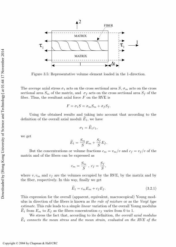
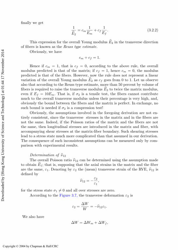
Figure 3.5: Representative volume element loaded in the 1-direction.

The average axial stress σ1 acts on the cross sectional area S, σm acts on the crosssectional area Sm of the matrix, and σf acts on the cross sectional area Sf of thefiber. Thus, the resultant axial force F on the RVE is

F = σ1S = σmSm + σfSf .

Using the obtained results and taking into account that according to thedefinition of the overall axial moduli E1, we have

σ1 = E1ε1,

we get

E1 =Sm

SEm +

Sf

SEf .

But the concentrations or volume fractions cm = vm/v and cf = vf/v of thematrix and of the fibers can be expressed as

cm =Sm

S, cf =

Sf

S,

where v, vm and vf are the volumes occupied by the RVE, by the matrix and bythe fiber, respectively. In this way, finally we get

E1 = cmEm + cfEf . (3.2.1)

This expression for the overall (apparent, equivalent, macroscopical) Young mod-ulus in direction of the fibers is known as the rule of mixture or as the Voigt typeestimate. This rule leads to a simple linear variation of the overall Young modulusE1 from Em to Ef as the fibers concentration cf varies from 0 to 1.

We stress the fact that, according to its definition, the overall axial modulusE1 connects the mean stress and the mean strain, evaluated on the RVE of the


Dow

nloa

ded

by [

Hon

g K

ong

Uni

vers

ity o

f Sc

ienc

e an

d T

echn

olog

y] a

t 01:

44 1

7 N

ovem

ber

2014


composite material. In the elasticity approach of the problem, the overall moduliwill be introduced in the same way!

Determination of E2

We now consider the overall Young modulus E2, in the direction transverseto the fibers. In the mechanics of the material approach, the same transverse stressσ2 is assumed to be applied to both the matrix and the fiber, as shown in Figure3.6. Such kind of hypotheses was first made by Reuss in 1929.

Figure 3.6: Representative volume element loaded in 2-direction.

The transverse strains εm and εf , in the matrix and in the fiber, respectively,are therefore

εm =σ2

Em, εf =

σ2

Ef.

The transverse direction over which on the average εm acts is approximately cmW ,whereas εf acts on cfW . Thus, the total transverse deformation is

ε2W = cmWεm + cfWεf ;

Hence, the mean transverse deformation ε2 becomes

ε2 = cmεm + cfεf .

Introducing here the stress-strains relations, we get

ε2 = cmσ2

Em+ cf

σ2

Ef.

Recognizing that according to its definition the overall moduli E2 must satisfythe material law

ε2 =1

E2

σ2,


Dow

nloa

ded

by [

Hon

g K

ong

Uni

vers

ity o

f Sc

ienc

e an

d T

echn

olog

y] a

t 01:

44 1

7 N

ovem

ber

2014


finally we get1

E2

= cm1

Em+ cf

1

Ef. (3.2.2)

This expression for the overall Young modulus E2 in the transverse directionof fibers is known as the Reuss type estimate.

Obviously, we have

cm + cf = 1.

Hence if cm = 1, that is cf = 0, according to the above rule, the overallmodulus predicted is that of the matrix; if cf = 1, hence cm = 0, the moduluspredicted is that of the fibers. However, now the rule does not represent a linearvariation of the overall Young modulus E2 as cf goes from 0 to 1. Let us observealso that according to the Reuss type estimate, more than 50 percent by volume offibers is required to raise the transverse modulus E2 to twice the matrix modulus,even if Ef = 10Em. That is, if σ2 is a tensile test, the fibers cannot contributemuch to the overall transverse modulus unless their percentage is very high, and,obviously the bound between the fibers and the matrix is perfect. In exchange, nosuch bound is needed if σ2 is a compression test!

Obviously, the assumptions involved in the foregoing derivation are not en-tirely consistent, since the transverse stresses in the matrix and in the fibers arenot the same. Indeed, if the Poisson ratios of the matrix and the fibers are notthe same, then longitudinal stresses are introduced in the matrix and fiber, withaccompanying shear stresses at the matrix-fiber boundary. Such shearing stresseslead to a stress state much more complicated than that assumed in our derivation.The consequence of such inconsistent assumptions can be measured only by com-parison with experimental results.

Determination of ν12

The overall Poisson ratio ν12 can be determined using the assumption madeto obtain E1; that is, supposing that the axial strains in the matrix and the fiberare the same, ε1. Denoting by ε2 the (mean) transverse strain of the RVE, ν12 isdefined by

ν12 = −ε2ε1,

for the stress state σ1 6= 0 and all over stresses are zero.

According to the Figure 3.7, the transverse deformation ε2 is

ε2 =∆W

W= −ν12ε1.

We also have

∆W = ∆Wm + ∆Wf ,


Dow

nloa

ded

by [

Hon

g K

ong

Uni

vers

ity o

f Sc

ienc

e an

d T

echn

olog

y] a

t 01:

44 1

7 N

ovem

ber

2014


Figure 3.7: Representative volume element loaded in 1-direction.

∆Wm and ∆Wf being the transverse displacements of the matrix and of the fiber,respectively. Consequently

∆Wm

W+

∆Wf

W= − ν12ε1.

Following the same procedure as in analysis for the overall transverse Youngmodulus E2, we assume that the transverse displacements ∆Wm and ∆Wf areapproximately

∆Wm = −Wcmνmε1 , ∆Wf = −Wcfνfε1,

−νmε1 and −νfε1 being the average transverse deformations of the matrix andof the fiber, respectively. Combining the last equations, we get

ν12 = cmνm + cfνf . (3.2.3)

The strength of materials rule leads to the mixture rule or to the Voigt typeestimate of the overall Poisson ratio ν12.

Determination of G12

The overall in-plane shear modulus G12 of a lamina is estimated in the me-chanics of materials approach by assuming a Reuss type hypothesis. It is supposedthat the same shear stress τ acts in the matrix and in the fiber. Denoting by γm

and γf , the shear strains in the matrix and fiber, respectively, we get

γm =1

µmτ , γf =

1

µfτ.

The loading is shown in Figure 3.8 and the deformations on microscopic scale inFigure 3.9. The total (mean) shear deformation γ is

γ =∆

W,


Dow

nloa

ded

by [

Hon

g K

ong

Uni

vers

ity o

f Sc

ienc

e an

d T

echn

olog

y] a

t 01:

44 1

7 N

ovem

ber

2014


Figure 3.8: Representative volume element loaded in shear.

MATRIX

MATRIX

FIBER

m

f

/2

Figure 3.9: Shear deformation of a representative volume element.

and we have∆ = ∆m + ∆f ,

∆m and ∆f being the horizontal displacements of the matrix and of the fiber,respectively. Denoting by γm and γf the shear strains in the matrix and fiber,respectively, we approximately get

∆m = cmWγm ∆f = cfW γf .

Hence,γ = cmγm + cfγf .

The overall in-plane shear modulus G12, connecting the mean strain γ andthe mean stress τ , is defined by

γ =1

G12

τ.

Thus, using the above formulas, we obtain

1

G12

= cm1

µm+ cf

1

µf. (3.2.4)


Dow

nloa

ded

by [

Hon

g K

ong

Uni

vers

ity o

f Sc

ienc

e an

d T

echn

olog

y] a

t 01:

44 1

7 N

ovem

ber

2014


Material Glass/Epoxy Carbon/EpoxyEf 70 234νf 0.17 0.2Em 2.85 3.8νm 0.33 0.33cf 0.66 0.6

Methods

Experimental

Mixture rules

E1 E2 G12 ν1249.40 18.00 7.80 0.22

47.16 7.77 2.95 0.224

E1 E2 G12 ν12151 9.3 6.2 0.32

141.8 9.2 3.5 0.25

Material Boron/EpoxyEf 413νf 0.2Em 4.10νm 0.35cf 0.70

Methods

Experimental

Mixture rules

E1 E2 G12 ν12237.8 13.3 5.5

290 26.7 12.2 0.245

Table 3.4: Experimental and calculated values of the overall elastic coefficients.

The strength of materials approach leads to a Reuss type estimation for theoverall in-plane shear modulus G12.

As in the case of E2, only for a fiber volume greater than 50 percent of thetotal volume does G12 rise to above twice µm even if µf = 10µm.

Using the data given by Barran and Loroze [3.9], we present in Table 3.4 themechanical characteristics of three fiber-reinforced composite materials, giving alsothe fiber concentrations. We also give the overall elastic coefficients experimentallydetermined and the values of the overall moduli calculated using the mixture rulesobtained by the strength of materials approach. The axial Young modulus E1 andthe transverse Poisson ratio ν12 are evaluated taking into account the Voigt typemixture rules (3.2.1), (3.2.2), and the transverse Young modulus E2 and the in-

plane transverse shear modulus G12 are obtained using the Reuss type mixturerules (2.3.3), (3.2.4). The axial and transverse Young moduli, as well as the shearmodulus are expressed in GPa = 109Pa.

Examining the above data, we can see that the calculated values of the overallaxial Young modulus E1 and those of the overall transverse Poisson ratio ν12 areacceptable as first approximations. However, the calculated values of the overalltransverse Young modulus E2 and those of the overall transverse shear modulusG12 are not acceptable, and cannot be used as a first approximation. Generally,we can say that much more powerful methods are necessary to evaluate and/orto bound the overall moduli as those obtained with the strength of materialsapproach.


Dow

nloa

ded

by [

Hon

g K

ong

Uni

vers

ity o

f Sc

ienc

e an

d T

echn

olog

y] a

t 01:

44 1

7 N

ovem

ber

2014

3.3. GLOBAL CONSTITUTIVE EQUATIONS 131

The above estimations are only examples of the type of mechanics of materialsapproaches that can be used to obtain approximate expression for the overallmoduli. Other assumptions of mechanical behavior lead to different estimationsfor the overall elastic moduli of the lamina.

The true significance of the Voigt and Reuss type estimates can be clarifiedonly by using the elasticity approach to get the overall stiffnesses. As we shallsee in Section 4.1, the Voigt and Reuss type estimations give universal-bounds forthe overall moduli. Generally, these estimates are the worst bounds that can bederived by the elastic approach.

We end this Section with some words concerning the approach named nettinganalysis (see Jones [3.2], Chapter 3, Section 3.3.1). The basic assumption in nettinganalysis is that the fibers provide all the longitudinal stiffness and the matrixprovide all the transverse and shear stiffness as well as the Poisson effect. Evenon the base of the above results furnished by the mechanics of material, we cansee that the assumptions made by the netting analysis must generally be rejected.In turn, the results due to the strength of materials approach must be carefullyanalyzed in light of the elasticity approach. Some important results of this analysiswill be presented in Chapter 4.

3.3 Global constitutive equations

As we have seen, a laminate is composed of two or more laminae boundedtogether to act as a structural element. The constituent laminae are oriented toproduce a structural element capable of resisting load in several directions. Thestiffness of such a composite body results from the properties of the constituentlaminae, as well as from their relative orientations. In the following, we present thebasic formulation of the classical lamination theory . The major difference betweenthis theory and the classical theory of homogeneous isotropic plates is in the formof the stress strain relationships of the lamina. Other elements of the theory such asthe deformation hypothesis, the equilibrium equation and the strain displacementrelationships are the same as those used in the classical plate theory.

Although the laminate is made up of multiple laminae, it is assumed, thatthe individual laminae are perfectly bounded together so as to behave as a unitary,nonhomogeneous, anisotropic plate. Interfacial slip is not allowed and the interfa-cial bounds are not allowed to deform in shear, which mean that the displacementacross laminae interfaces are assumed to be continuous. The assumptions implythat deformation hypothesis from the classical homogeneous plate theory can beused for the laminated composite plate.

Figure 3.10 shows the coordinate system to be used in developing the lami-nated plate analysis. The x1, x2, x3 coordinate system is assumed to have its originon the middle surface of the plate, so that the x1x2 planes lie in the middle plane.The components of the displacement u are u1, u2, u3 and they depend on x1, x2, x3.Frequently, x1, x2, x3 are denoted by x, y, z and u1, u2, u3 by u, v, w.


Dow

nloa

ded

by [

Hon

g K

ong

Uni

vers

ity o

f Sc

ienc

e an

d T

echn

olog

y] a

t 01:

44 1

7 N

ovem

ber

2014


Figure 3.10: Coordinate system for laminated plate.

The basic assumptions made in the frame-work of the classical compositelaminate theory are the following:

(1) The plate consists of orthotropic laminae bounded together, with theprincipal material axes of the orthotropic laminae oriented at arbitrary directionwith respect to the x1, x2 axes.

(2) The thickness h of the plate is much smaller than the length along theplate edges a and b.

(3) The displacements u1, u2, u3 are small compared with the plate thicknessh.

(4) The in-plane strains ε11, ε22, ε12 are small compared with unity.(5) Transverse shear strains ε13 and ε23 are negligible.(6) The transverse normal strain ε33 is negligible.(7) The normal stress σ33 is small in comparison with the other stress com-

ponents.(8) The transverse shear stresses σ13 and σ23 vanish on the plate surfaces

x3 = ±h2 .

(9) Each lamina obeys the reduced stress-strain relation corresponding toplane stress state.

The assumption (2) stresses the fact that we develop here the classical thinlamination theory. The assumptions (3) and (4) show that the theory refers tosmall deformations, that is it is geometrically linear. The assumptions (5) and (6)express the classical Love-Kirchhoff hypothesis, known also as the hypothesis ofplane sections: any normal to the middle surface remains straight and normal tothe deformed middle surface, and at the same time, its magnitude rests constantduring the deformation. The assumptions (7), (8) and (9) express the fact thestresses σ13, σ23 and σ33 are assumed to be small in comparison with the stressesσ11, σ22 and σ12. That is, as is stated in the assumption (9), the stresses σ11, σ22 andσ12 and the strains ε11, ε22 and ε12 can be related using the reduced stress-strainrelatives corresponding to the plane stress state of the laminae. Since the assumedhypotheses are similar to those used in the classical Love-Kirckhhoff theory of ho-mogeneous isotropic thin plate, the classical lamination theory of composite lami-nates inherits all internal contradictions and inconsistencies of the Love-Kirckhhoff


Dow

nloa

ded

by [

Hon

g K

ong

Uni

vers

ity o

f Sc

ienc

e an

d T

echn

olog

y] a

t 01:

44 1

7 N

ovem

ber

2014


theory. This observation concerns all of the internal contradiction existing betweenthe assumptions (7), (8) and (9): though σ13, σ23 and σ33 are not vanishing, weuse the reduced stress-strain relations corresponding to vanishing σ13, σ23 and σ33.Obviously, the seriousness and consequences of these inconveniences can be estab-lished only by studying the implication of the theory based on the assumptions(1)-(9). For this purpose, we must first develop the classical lamination theory,using the supposed hypothesis.

From assumption (6), we obtain

ε33(x1, x2, x3) =∂u3

∂x3(x1, x2, x3) = 0.

Consequently, the normal displacement u3(x1, x2, x3) depends only on x1 and x2;i.e.

u3 = U3(x1, x2). (3.3.1)

From the assumption (5), we get

2ε13(x1, x2, x3) =∂u1

∂x3(x1, x2, x3) +

∂u3

∂x1(x1, x2, x3) = 0,

2ε23(x1, x2, x3) =∂u2

∂x3(x1, x2, x3) +

∂u3

∂x2(x1, x2, x3) = 0.

From here, according to (3.3.1), the displacements u1(x1, x2, x3) andu2(x1, x2, x3) depend linearly on x3; i.e.

u1 = U1(x1, x2) − x3∂U3(x1, x2)

∂x1, u2 = U2(x1, x2) − x3

∂U3(x1, x2)

∂x2. (3.3.2)

In the above relations, U3(x1, x2) is the normal displacement of the middle surface,and U1(x1, x2), U2(x1, x2) characterize the tangential displacement of the samesurface.

From (3.3.2), we obtain the following expressions for the non-vanishing straincomponents ε11, ε22, ε33 :

εαβ = eαβ + x3kαβ , α, β = 1, 2, (3.3.3)

where

eαβ = eαβ(x1, x2) =1

2(∂Uα

∂xβ+∂Uβ

∂xα) =

1

2(Uα,β + Uβ,α) (3.3.4)

describe the deformation of the middle surface x3 = 0, and

kαβ(x1, x2) = kβα(x1, x2) = − ∂U3

∂xα∂xβ= −U3,αβ (3.3.5)

are the curvatures of the same surface.


Dow

nloa

ded

by [

Hon

g K

ong

Uni

vers

ity o

f Sc

ienc

e an

d T

echn

olog

y] a

t 01:

44 1

7 N

ovem

ber

2014


In the following, the Greek indices take the values 1 and 2.For later use, we introduce the following matrix notations:

[σ] =

σx

σy

σxy

=

σ11

σ22

σ12

, [ε] =

εx

εy

γxy

=

ε11ε222ε12

,

[e] =

e11e222e12

, [k] =

k11

k22

2k12

(3.3.6)

Thus from (3.3.3) we get

[ε] = [e] + x3 [k] . (3.3.7)

In Figure 3.11, we present the geometry of an N-layered laminate, clarifying inthis way the relations which will be used in what follows. Occasionally, to simplifysome formulas, we shall use the notation x3 = z.

Figure 3.11: Geometry of an N -layered laminate.

The k-th lamina occupies the domain defined by

zk−1 < z < zk, k = 1, ..., N with x3 = z.

Obviously, z0 = −h2 and zN = h

2 .We return now to assumption (9). According to this hypothesis, in each

lamina the reduced and transformed stress-strain relation (3.1.15) is valid. Hence,we have

σx

σy

σxy

k

=

Q11 Q12 Q16

Q12 Q22 Q26

Q16 Q26 Q66

k

εx

εy

γxy

k

for k = 1, .., N. (3.3.8)

Using the simplified matrix notation (3.3.6), we get

[σ]k =[Q]k[εk] for zk−1 < x3 = z < zk and k = 1, .., N. (3.3.9)


Dow

nloa

ded

by [

Hon

g K

ong

Uni

vers

ity o

f Sc

ienc

e an

d T

echn

olog

y] a

t 01:

44 1

7 N

ovem

ber

2014


Since according to (3.3.7), eαβ and kαβ depend on x1,x2 only, the last equa-tion becomes

[σ]k =[Q]k[e] + x3

[Q]k[k] for zk−1 < x3 = z < zk and k = 1, .., N. (3.3.10)

The last equation expresses the plane stress σ11, σ22, σ12 in the k-th layer, interms of the laminate middle surface strains and curvatures.

Expanded, the equation (3.3.10) becomes

σ11

σ22

σ12

k

=

Q11 Q12 Q16

Q12 Q22 Q26

Q16 Q26 Q66

k

e11e222e12

+x3

Q11 Q12 Q16

Q12 Q22 Q26

Q16 Q26 Q66

k

k11

k22

2k12

(3.3.11)for zk−1 < x3 = z < zk and k = 1, .., N.

In the above equations, k denotes the k-th lamina, (σαβ)k, α, β = 1, 2 are thestress in the k-th lamina, (Qij)k, i, j = 1, 2, 6 are the transformed reduced stiffnessof the k-th lamina, zk−1 and zk are the distances from the middle surface to theinner and to the outer surfaces of the k-th lamina, respectively, and N is the totalnumber of the laminae.

We recall that the reduced stiffness Qij , i, j = 1, 2, 6 depend on θ, the anglemade by the fibers with axis Ox1, and we have

(Qij)k = Qij(θk) for zk−1 < x3 = z < zk and k = 1, ...N, (3.3.12)

θk representing the angle made by the fibers in the k-th lamina and the body axisx1.

Since (Qij)k can be different for each lamina of the laminate, the stressvariation through the thickness is not necessarily linear, even though the strainvariation is linear, as can be seen by examining equation (3.3.3).

In the laminated plate analysis, it is convenient to use the forces Nαβ andthe moments Mαβ per unit length, defined by the following relations:

Nαβ = Nβα =

∫ h2

−h2

σαβdx3, Mαβ = Mβα =

∫ h2

−h2

x3σαβdx3, α, β = 1, 2. (3.3.13)

Let us observe that usually N11, N12 = N21, N22 are denoted by Nxx, Nxy =Nyx andNyy, respectively, and alsoM11,M12 = M21,M22 are denoted byMxx,Mxy

= Myx,Myy, respectively.According the relation (3.3.13)1 N11, N12, N22 are forces per unit length of

the cross-section. The mechanical meaning of these force resultants are shown inthe Figure 3.12.

Similarly, equation (3.3.13)2 shows that M11,M12,M22 are moments per unitlength of the cross-section. In Figure 3.13 is shown the mechanical meaning ofthese moment resultants.


Dow

nloa

ded

by [

Hon

g K

ong

Uni

vers

ity o

f Sc

ienc

e an

d T

echn

olog

y] a

t 01:

44 1

7 N

ovem

ber

2014


Figure 3.12: In-plane forces on a flat laminate.

Figure 3.13: Moments on a flat laminate.

The relations (3.3.13) show that these force and moments resultants do notdepend on x3, but are functions of x1 and x2, the in the plane coordinates of thelaminate middle surface.

In more detail, the defining equations (3.3.13) can be written as

[N ] =

N11

N22

N12

=

N∑

k=1

∫ zk

zk−1

σ11

σ22

σ12

k

dz;

[M ] =

M11

M22

M12

=

N∑

k=1

∫ zk

zk−1

z

σ11

σ22

σ12

k

dz. (3.3.14)

The integrations indicated in these equations can be rearranged to take ad-vantage of the fact that the stiffness matrix for a lamina is constant within eachlamina. Thus, substituting the stress-strain relations (3.3.11) and taking into ac-


Dow

nloa

ded

by [

Hon

g K

ong

Uni

vers

ity o

f Sc

ienc

e an

d T

echn

olog

y] a

t 01:

44 1

7 N

ovem

ber

2014


count the fact that eαβ and kαβ do not depend on x3 = z, we get

[N ] =

{N∑

k=1

[Q]k

∫ zk

zk−1

dz

}[e] +

{N∑

k=1

[Q]k

∫ zk

zk−1

zdz

}[k],

[M ] =

{N∑

k=1

[Q]k

∫ zk

zk−1

zdz

}[e] +

{N∑

k=1

[Q]k

∫ zk

zk−1

z2dz

}[k].

Finally, these equations can be written as

[N ] =

N11

N22

N12

=

A11 A12 A16

A21 A22 A26

A61 A62 A66

e11e222e12

+

B11 B12 B16

B21 B22 B26

B61 B62 B66

k11

k22

2k12

,

[M ] =

M11

M22

M12

=

B11 B12 B16

B21 B22 B26

B61 B62 B66

e11e222e12

+

D11 D12 D16

D21 D22 D26

D61 D62 D66

k11

k22

2k12

,

(3.3.15)where the coefficients Aij , Bij , Dij , i, j = 1, 2, 6 are defined by

Aij = Aji =N∑

k=1

(Qij)k(zk − zk−1),

Bij = Bji = 12

N∑k=1

(Qij)k(z2k − z2

k−1),

Dij = Dji = 13

N∑k=1

(Qij)k(z3k − z3

k−1).

(3.3.16)

Introducing the symmetric 3 × 3 matrices

[A]=

A11 A12 A16

A12 A22 A26

A61 A26 A66

, [B]=

B11 B12 B16

B12 B22 B26

B61 B26 B66

, [D]=

D11 D12 D16

D12 D22 D26

D61 D26 D66

(3.3.17)the equations (3.1.15) can be expressed in a concentrated matrix form

[N ] = [A][e] + [B][k], [M ] = [B][e] + [D][k] (3.3.18)

the 3 × 1 matrixes [e] and [k] being defined by equation (3.3.6)3,4.Also, the system (3.3.18) can be replaced by the following matrix equation:

N11

N22

N12

M11

M22

M12

=

A11 A12 A16

A21 A22 A26

A61 A62 A66

B11 B12 B16

B21 B22 B26

B61 B62 B66

B11 B12 B16

B21 B22 B26

B61 B62 B66

D11 D12 D16

D21 D22 D26

D61 D62 D66

e11e222e12k11

k22

2k12

. (3.3.19)


Dow

nloa

ded

by [

Hon

g K

ong

Uni

vers

ity o

f Sc

ienc

e an

d T

echn

olog

y] a

t 01:

44 1

7 N

ovem

ber

2014


This equation describing the global behavior of the laminate, can be expressedin the concentrated form

[NM

]=

[A BB D

] [ek

]= [E]

[ek

]. (3.3.20)

The 6 × 6 symmetric matrix [E] is the global laminate stiffness matrix.The coefficients Aij are called extensional stiffnesses, the coefficients Bij de-

scribe the coupling stiffness, and the coefficients Dij are called bending stiffnesses.The presence of the coefficients Bij implies coupling between bending and extensionof a laminate. That is, it is impossible to pull on a laminate that has non-vanishingBij terms, without at the same time bending and/or twisting the laminate. Thus,an extensional force results not only in extensional deformation of the middle sur-face, but also in twisting and/or bending of the laminate. Also, such a laminatecannot be subjected to a moment without at the same time being subjected toan extension of the middle surface. The experiments made with laminates confirmthese theoretical predictions. In spite of this fact, in the stability analysis of lam-inates, this coupling is generally neglected and we shall discuss this question inChapter 7.

It is easy to see that the matrix equation (3.3.19) can be written in thefollowing tensorial or component form, very useful in many problems

Nαβ = Aαβγϕeγϕ +Bαβγϕkγϕ,Mαβ = Bαβγϕeγϕ +Dαβγϕkγϕ, α, β, γ, ϕ = 1, 2.

(3.3.21)

The coefficients of these equations can be expressed simply and obviously byusing the quantities A11, ..., D66. For instance, we have

A1111 = A11 , A1122 = A2211 = A12,A1112 = A1121 = A1211 = A2111 = A16,A1212 = A1221 = A2112 = A2121 = A66, ...,B1111 = B11 , B1122 = B2211 = B12,B1112 = B1121 = B1211 = B2111 = B16,B1212 = B1221 = B2112 = B2121 = B66, ...,D1111 = D11 , D1122 = D2211 = D12,D1112 = D1121 = D1211 = D2111 = D16,D1212 = D1221 = D2112 = D2121 = D66, ....

(3.3.22)

It is also clear that the following symmetry relations take place

Aαβγϕ = Aβαγϕ = Aαβϕγ = Aγϕαβ ,

Bαβγϕ = Bβαγϕ = Bαβϕγ = Bγϕαβ ,

Dαβγϕ = Dβαγϕ = Dαβϕγ = Dγϕαβ .

(3.3.23)


Dow

nloa

ded

by [

Hon

g K

ong

Uni

vers

ity o

f Sc

ienc

e an

d T

echn

olog

y] a

t 01:

44 1

7 N

ovem

ber

2014


We stress the fact that the constitutive coefficients Aαβγϕ, Bαβγϕ, Dαβγϕ

have the same symmetries as the elasticities of a linearly elastic material. As weshall see later, this property will have important consequences.

We assume now that the global constitutive equation (3.3.20) is invertible. InChapter 7, we shall see that this property is always true if the initial configurationof the laminate is (locally) stable.

In order to express [e] and [k] in terms of [N ] and [M ], we rewrite (3.3.20) as

[N ] = [A][e] + [B][k], [M ] = [B][e] + [D][k]. (3.3.24)

From the first equation we get

[e] = [A]−1[N ] − [A]−1[B][k]. (3.3.25)

Substitution of (3.3.25) in (3.3.24)2 gives

[M ] = [B][A]−1[N ] − [B][A]−1[B][k] + [D][k]. (3.3.26)

Equation (3.3.25) and (3.3.26) give a partially inverted form of the equation(3.3.20) [

eM

]=

[A∗ B∗

C∗ D∗

] [Nk

], (3.3.27)

with

[A∗] = [A]−1, [B∗] = − [A]

−1[B] , [C∗] = [B][A]−1, [D∗] = [D] − [B][A]−1[B].

(3.3.28)Now, using (3.3.27) for [k], we get

[k] = [D∗]−1[M ] − [D∗]−1[C∗][N ]. (3.3.29)

Introducing (3.3.29) in (3.3.25), we obtain

[e] ={[A∗] − [B∗][D∗]−1[C∗]

}[N ] + [B∗][D∗]−1[M ]. (3.3.30)

Finally, (3.3.29) and (3.3.30) lead to the following inverted global constitutiveequation. [

ek

]=

[A′ B′

C ′ D′

] [NM

]= [E]

−1

[NM

], (3.3.31)

where[A′] = [A∗] − [B∗][D∗]−1[C∗],[B′] = [B∗][D∗]−1,[C ′] = −[D∗]−1[C∗] = [B′]ᵀ = [B′],[D′] = [D∗]−1.

(3.3.32)

The last results show that the 6 × 6 global compliance matrix [E]−1 is sym-metric. This is an obvious result, since if the global stiffness matrix [E] beingsymmetric, its inverse, if it exists, must also be symmetric.


Dow

nloa

ded

by [

Hon

g K

ong

Uni

vers

ity o

f Sc

ienc

e an

d T

echn

olog

y] a

t 01:

44 1

7 N

ovem

ber

2014


3.4 Special classes of laminates

This Section considers special classes of laminates for which the stiffnessescan easily be calculated. The special classes will be presented in increasing orderof complexity.

1. Single - layered configurationsFor a single isotropic layer with material properties E, ν and thickness h,

equations (3.3.16) give

A11 = A22 =Eh

1 − ν2≡ A, A12 = νA , A16 = A26 = 0 , A66 =

1 − ν

2A , Bij = 0 ,

D11 = D22 =Eh3

12(1 − ν2)≡ D , D12 = νD , D16 = D26 = 0 , D66 =

1 − ν

2D.

(3.4.1)In order to obtain the above relations, we must use the equations (3.1.6),

supposing an isotropic material.From (3.4.1), we can conclude that the resultant forces depend only on the

in-plane strains of the laminate middle surface, and the resultant moments dependonly on the curvatures of the middle surface. There is no coupling. The constitutiveequations become

N11

N22

N12

=

A νA 0νA A 00 0 (1 − ν)A

2

e11e222e12

,

M11

M22

M12

=

D νD 0νD D 00 0 (1 − ν)D

2

k11

k22

2k12

.

(3.4.2)

In particular, we have

D =h2

12A. (3.4.3)

For a simple specially orthotropic layer of thickness h the lamina stiffnessesare given by equation (3.1.6). Hence, according to (3.3.10), the laminate stiffnessesare

A11 = hQ11 , A12 = hQ12 , A22 = hQ22 , A16 = A26 = 0 , A66 = hQ66 ,

Bij = 0,

D11 =h3

12Q11 , D12 =

h3

12Q12 , D22 =

h3

12Q22 , D16 = D26 = 0 , D66 =

h3

12Q66.

(3.4.4)


Dow

nloa

ded

by [

Hon

g K

ong

Uni

vers

ity o

f Sc

ienc

e an

d T

echn

olog

y] a

t 01:

44 1

7 N

ovem

ber

2014

3.4. SPECIAL CLASSES OF LAMINATES 141

Again, the resultant forces depend only on the in-plane strains, and the re-sultant moments depend only on the curvatures. There is no coupling. The con-stitutive equation becomes

N11

N22

N12

=

A11 A12 0A12 A22 00 0 A66

e11e222e12

,

M11

M22

M12

=

D11 D12 0D12 D22 00 0 D66

k11

k22

2k12

.

(3.4.5)

2. Symmetric laminate

For laminates that are symmetric in both geometry and material propertiesabout the middle surface, the general stiffness equations (3.3.16) simplify consid-erably. Because of the symmetry of the transformed stiffnesses (Qij)k and of thethicknesses hk, it can be shown that all coupling stiffness Bij of the laminate arezero. There is no coupling. Obviously such laminates are much easier to analyzethan laminates with coupling. Consequently, symmetric laminates are commonlyused unless special circumstances require an unsymmetrical laminate possessingthe coupling property.

The constitutive equations for a symmetric laminate are

N11

N22

N12

=

A11 A12 A16

A12 A22 A26

A16 A26 A66

e11e222e12

,

M11

M22

M12

=

D11 D12 D16

D12 D22 D26

D16 D26 D66

k11

k22

2k12

.

(3.4.6)

In the following, we shall present some special cases of symmetric laminates,determining the stiffness Aij and Dij in each case.

For symmetric laminates with multiple isotropic layers, multiple isotropiclaminae of various thicknesses are arranged symmetrically about the middle surfacefrom both a geometric and a material property standpoint. The resulting laminatedoes not exhibit coupling between extension and bending. The extensional andbending stiffnesses are calculated from the equations (3.3.16), where, according to(3.1.6), and assuming an isotropic material, for the k-th layer, we get

(Q11)k = (Q22)k =Ek

1 − ν2k

, (Q16)k = (Q26)k = 0 ,

(Q12)k =νkEk

1 − ν2k

, (Q66)k =Ek

2(1 + ν2k). (3.4.7)


Dow

nloa

ded

by [

Hon

g K

ong

Uni

vers

ity o

f Sc

ienc

e an

d T

echn

olog

y] a

t 01:

44 1

7 N

ovem

ber

2014


In these equations, Ek and νk are the Young’s modulus and the Poisson’sratio for the k-th lamina.

It is easy to see that

A11 = A22 , A16 = A26 = 0 , D11 = D22 , D16 = D26 = 0. (3.4.8)

Hence, the constitutive equations becomeN11

N22

N12

=

A11 A12 0A12 A11 00 0 A66

e11e222e12

,

M11

M22

M12

=

D11 D12 0D12 D11 00 0 D66

k11

k22

2k12

.

(3.4.9)

A symmetric laminate with multiple specially orthotropic layers is made oforthotropic layers that have their principal material directions aligned with thelaminate axes, and the layers (laminae) having various thicknesses, are arrangedsymmetrically about the middle surface both from a geometric and a materialproperty standpoint. The stiffnesses of the laminate are calculated from the generalequations (3.3.16), whereas, according to (3.1.6) for the k-th lamina

(Q11)k =Ek

1

1 − νk12ν

k21

, (Q12)k =νk21E

k1

1 − νk12ν

k21

, (Q22)k =Ek

2

1 − νk12ν

k21

,

(Q66)k = Gk12 , (Q16)k = (Q26)k = 0 , (3.4.10)

Ek1 , E

k2 , ν

k12, ν

k21 and Gk

12 being the engineering material constants of the k-th spe-cially orthotropic lamina.

Because (Q16)k and (Q26)k are zero, it is easy to see that A16, A26, D16 andD26 vanish; i.e.

A16 = A26 = 0 , D16 = D26 = 0. (3.4.11)

Also, because of symmetry, the coupling stiffnesses Bij are all zero; i.e.

Bij = 0. (3.4.12)

Hence, the constitutive equation for the laminate takes the formN11

N22

N12

=

A11 A12 0A12 A22 00 0 A66

e11e222e12

,

M11

M22

M12

=

D11 D12 0D12 D22 00 0 D66

k11

k22

2k12

.

(3.4.13)


Dow

nloa

ded

by [

Hon

g K

ong

Uni

vers

ity o

f Sc

ienc

e an

d T

echn

olog

y] a

t 01:

44 1

7 N

ovem

ber

2014


Taking into account the above equations, this type of laminate could be calledspecially orthotropic laminate in analogy to a special orthotopic lamina.

A regular symmetric cross-ply laminate represents a very common special caseof symmetric laminates with multiple specially orthotropic laminae (layers). Theregular symmetric cross-ply laminate occurs when the laminae are all of the samethickness and material properties, and their major principal material direction(that is, the fiber directions) alternate at 00 or 900 with respect to the laminate(body) axes, for examples (00/900/00) as in Figure 3.14.

Figure 3.14: Exploded (unbounded) view of a three-layered regular symmetriccross-ply laminate.

The regular symmetric cross-ply laminate must have an odd number of layersif we wish to satisfy the symmetric requirement by which coupling between bendingand extension is eliminated. Cross-ply laminates with an even number of layersare not symmetric and will be discussed a little later on.

Before analyzing other special classes of laminates, let us say a few wordsabout the logic to establish various stiffnesses.

For simplicity, we denote x3 by z; i.e. x3 = z.Let us consider the extensional stiffnesess

Aij =N∑

k=1

(Qij

)k(zk − zk−1) ,

given by equation (3.3.16)1.Since zk − zk−1 > 0 for k = 1, ..., N , the above equation shows that the only

way to have an Aij zero is either for all(Qij

)k

to be zero, or for some of the(Qij

)k

to be a negative and some positive, so that the sum of their products withtheir respective thicknesses be zero. From equation (3.1.17) giving the transformedreduced stiffnesses Qij , follows that Q11 , Q12 , Q22 and Q66 are positive, since all


Dow

nloa

ded

by [

Hon

g K

ong

Uni

vers

ity o

f Sc

ienc

e an

d T

echn

olog

y] a

t 01:

44 1

7 N

ovem

ber

2014


trigonometrical functions are involved with even powers and Q11 , Q12 , Q22 , Q66

are positive. Thus, A11 , A12 , A22 and A66 are all positive since the thicknessesof the laminae are obviously positive. However, (Q16)k and (Q26)k are zero forlamina orientation of 00 or 900 to the laminate axes. Thus, A16 and A26 are zerofor laminates made of orthotropic laminae oriented at either 00 or 900 to thelaminate axes.

Next, we consider the coupling stiffnesses

Bij =1

2

N∑

k=1

(Qij)k

(z2k − z2

k−1

),

given by equation (3.3.16)2.It is easy to see that if the cross-ply laminate is symmetric about the middle

surface, then all the Bij vanish.Finally, we consider the bending stiffnesses

Dij =1

3

N∑

k=1

(Qij)k

(z3k − z3

k−1

),

given by equation (3.3.16)3.Since z3

k − z3k−1 > 0 and

(Q11

)k,(Q12

)k,(Q22

)k,(Q66

)k> 0, it results that

D11 , D12 , D22 and D66 are positive. Also(Q16

)k

and(Q26

)k

are zero for laminae

having principal material property orientation of 00 or 900 with respect to thelaminate coordinates. Thus, D16 and D26 also vanish.

Summing up, we can say that the status of the extensional and bendingstiffnesses is the same.

As we have seen, a laminate of multiple generally orthotropic layers that aresymmetrically disposed about the middle surface exhibits no coupling betweenbending and extension; that is the Bij are zero. Therefore, the force and momentsresultants are given by equation (3.4.6) There, all the Aij and Dij are requiredbecause of forces and shearing strains, shearing force and normal strains, normalmoments and twist, and twisting moment and normal curvatures coupling betweennormal forces N11, N12 and shearing strains e12, shearing force N12 and normalstrains e11, e22, normal moments M11,M22 and twist k12 and twisting moment M12

and normal curvatures k11, k22. Such coupling is evidenced by the A16, A26, D16

and D26 stiffnesses.A special subclass of this class of symmetric laminates is the regular symmet-

ric angle-ply laminate. Such laminates have orthotropic laminae of equal thick-nesses. The adjacent laminae have opposite signs of angle of orientation of theprincipal material properties with respect to the laminates axes, for example+α/− α/+ α as in Figure 3.15.

For symmetry, there must be an odd number of layers.The aforementioned coupling that involves A16 , A26 , D16 and D26 takes a

special form for symmetric angle-ply laminates. Those stiffnesses can be shown to


Dow

nloa

ded

by [

Hon

g K

ong

Uni

vers

ity o

f Sc

ienc

e an

d T

echn

olog

y] a

t 01:

44 1

7 N

ovem

ber

2014


Figure 3.15: Exploded (unbounded) view of a three-layered regular symmetricangle-ply laminate.

be largest when N = 3 (the lowest N for which this class of laminates exists) anddecrease in proportion to 1/N as N increases

A16 =

N∑

k=1

(Q16)k (zk − zk−1) andD16 =1

3

N∑

k=1

(Q16)k

(z3k − z3

k−1

),

obviously, A16 and D16 are sums of terms of alternating signs since

(Q16)+α = −(Q16)−α. (3.4.14)

Consequently, for many layered symmetric angle-ply laminates, the values of A16 ,A26 , D16 and D26 can be quite small when compared to the other Aij and Dij ,respectively.

3. Antisymmetric laminatesAs we have seen, symmetry of a laminate about a middle surface is generally

desired to avoid coupling between bending and extension. However, many engi-neering applications of laminated composite require antisymmetric laminates toachieve design requirements.

The general class of antisymmetric laminates has an even numbers of layersif adjacent laminae have alternating signs of the principal material directions withrespect to the laminate axes. In addition, each pair of laminae must have the samethickness.

It can be shown that in the case of an antisymmetric laminate

A16 = A26 = D16 = D26 (3.4.15)

since(Q16)α = −(Q16)−α , (Q26)α = −(Q26)−α , (3.4.16)


Dow

nloa

ded

by [

Hon

g K

ong

Uni

vers

ity o

f Sc

ienc

e an

d T

echn

olog

y] a

t 01:

44 1

7 N

ovem

ber

2014


where the above symbols represent the corresponding transformed reduced stiff-nesses in the laminae with the orientation α and −α of the fibers.

For general antisymmetric laminates, all coupling stiffnesses are non-vanishing.Hence, the constitutive equation (3.3.15) becomeN11

N22

N12

=

A11 A12 0A12 A22 00 0 A66

e11e222e12

+

B11 B12 B16

B12 B22 B26

B16 B26 B66

k11

k22

2k12

,

M11

M22

M12

=

B11 B12 B16

B12 B22 B26

B16 B26 B66

e11e222e12

+

D11 D12 0D12 D22 00 0 D66

k11

k22

2k12

.

(3.4.17)We discuss now two important subclasses of antisymmetric laminates.An antisymmetric cross-ply laminate consists of an even number of orthotropic

laminae laid down on each other with principal material directions alternating at00 and 900 to the laminate axes, as in the example given in Figure 3.16.

Figure 3.16: Exploded (unbounded) view of a two-layered regular antisymmetriccross-ply laminate.

The antisymmetric cross-ply laminates do not have non-zero A16 , A26 , D16 ,D26, but do have coupling between extension and bending. More precisely

A16 = A26 = 0 , D16 = D26 = 0 , B11 = −B22 , B12 = B16 = B26 = B66 = 0.(3.4.18)

Hence, the constitutive equations of the antisymmetric cross-ply laminates becomeN11

N22

N12

=

A11 A12 0A12 A22 00 0 A66

e11e222e12

+

B11 0 00 −B11 00 0 0

k11

k22

2k12

,

M11

M22

M12

=

B11 0 00 −B11 00 0 0

e11e222e12

+

D11 D12 0D12 D22 00 0 D66

k11

k22

2k12

.

(3.4.19)


Dow

nloa

ded

by [

Hon

g K

ong

Uni

vers

ity o

f Sc

ienc

e an

d T

echn

olog

y] a

t 01:

44 1

7 N

ovem

ber

2014


A regular antisymmetric cross-ply laminate is a special case, which has lam-inae of equal thickness. This type of laminate is common because of simplicity offabrication.

It can be shown that the coupling stiffness B11 of an antisymmetric cross-plylaminate approaches zero as the number of layers increases, for a fixed laminatethickness.

An antisymmetric angle-ply laminate has laminae oriented at +α degrees tothe laminate coordinate axes on one side of the middle surface and the correspond-ing equal thickness laminae on the other side is oriented at −α degrees. A simpleexample is given in Figure 3.17.

y = x

x = x1

2

Figure 3.17: Exploded (unbounded) view of a two-layered regular antisymmetricangle-ply laminate.

A regular antisymmetric angle-ply laminate has all laminae of the same thick-nesses.

It can be shown that for an antisymmetric angle-ply laminate, the followingstiffnesses are vanishing:

A16 = A26 = 0 , B11 = B12 = B22 = 0 , D16 = D26 = 0. (3.4.20)

Consequently, the global constitutive equations become

N11

N22

N12

=

A11 A12 0A12 A22 00 0 A66

e11e222e12

+

0 0 B16

0 0 B26

B16 B26 0

k11

k22

2k12

,

M11

M22

M12

=

0 0 B16

0 0 B26

B16 B26 0

e11e222e12

+

D11 D12 0D12 D22 00 0 D66

k11

k22

2k12

.

(3.4.21)It can be shown for a fixed laminate thickness that the coupling stiffnesses

B16 and B26 tend towards zero as the number of layers in the laminate increases.Summing up the presented results, concerning some special classes of fiber-

reinforced composite laminates, we can say the following:


Dow

nloa

ded

by [

Hon

g K

ong

Uni

vers

ity o

f Sc

ienc

e an

d T

echn

olog

y] a

t 01:

44 1

7 N

ovem

ber

2014


(1) Simple layer laminates with a reference surface, at the middle surface donot exhibit coupling between extension and bending.

(2) Multilayered laminates, in general, develop coupling between extensionand bending.

(3) The coupling is influenced by the geometrical as well as by the materialproperties of the laminae.

(4) There exist combinations of the material properties and geometrical char-acteristics for which there is no coupling between extension and bending.

(5) The elastic symmetry of the laminae (transversally isotropy, orthotropy)is not necessarily conserved in the laminate.

(6) Moreover, the symmetries can be increased, decreased or remain the same.

(7) The symmetry properties of the three stiffness matrices [A], [B] and [D]need not be the same, and are generally different.

We stress the fact that the fundamental concept of coupling between exten-sion and bending must be well understood, because there exists many applicationsof the composite laminates where the neglect of the coupling can be catastrophic.Considering coupling is the key to the correct analysis of eccentrically stiffenedplates.

The procedure to describe a laminate by use of individual layer thicknesses,principal material property orientations, and overall sequence can be quite in-volved. However, all pertinent parameters can be represented in a simple way ifone uses the following stacking sequence terminology.

For regular (equal thickness layers) laminates, a listing of layers and their ori-entation suffices, for example, [00/900/450]. Let us observe that only the principalmaterial direction orientations need to be given.

For irregular (when the layers do not have the same thickness) laminates, anotation of layers’ thickness must be added to the previous notation, for example,[00/h1/90

0/h2/450/h3].

For symmetric laminates, the simplest representation of the laminate [00/900/450/450/900/00] is [00/900/450] sym.

We shall discuss now in greater details the relation by which the cross-plylaminate stiffnesses can be expressed.

We recall that a cross-ply laminate has N unidirectionally reinforced or-thotropic layers with the principal material directions alternatingly oriented at00and 900 with respect to the laminate coordinate axes. The fiber direction ofthe odd -numbered layers is the x1 direction of the laminate. The fiber directionof the even-numbered layers is the x2 direction of the laminate. We assume thatall odd-numbered layers have the same thickness, all even-numbered layers havealso equal thicknesses but the odd and even numbered layers do not necessarilyhave the same thickness. For this special but important case for applications, twogeometrical parameters are important:

(1) N, the total number of layers,and


Dow

nloa

ded

by [

Hon

g K

ong

Uni

vers

ity o

f Sc

ienc

e an

d T

echn

olog

y] a

t 01:

44 1

7 N

ovem

ber

2014


(2) m, the ratio of the total thicknesses of odd numbered layers to the totalthickness of the even-numbered layers, called cross-ply ratio. Hence,

m =

∑k=odd

hk

∑k=even

hk. (3.4.22)

For instance, for a five-layered cross-ply laminate, which has a lamination or stack-ing sequence [00/h1/90

0/2h1/00/2h1/90

0/2h1/00/h1], we get

m =h1 + h1 + h1

2h1 + 2h1= 3/4.

Let us observe that the cross-ply ratio m has a specific meaning only whenthe laminae (layers) have alternating 00 and 900 orientation!

Tsai (see Jones [3.2], Chapter 4) has shown that the laminate stiffnessesAij , Bij and Dij for cross-ply laminates with odd or even numbers of layers, canbe expressed in terms of m and N . In addition, Tsai uses the stiffness ratio

f = Q22/Q11 = E1/E2 6 1 (3.4.23)

of principal lamina stiffnesses.

Tsai has obtained the following expressions for the stiffnesses:

Symmetric cross-ply laminates (N odd).

A11 =m+ f

1 +mhQ11 , A12 = hQ12 , A22 =

1 +mf

1 +mhQ11 =

1 +mf

m+ fA11,

A16 = A26 = 0 , A66 = hQ66 , Bij = 0,

D11 =(f − 1)p+ 1

12h3Q11 =

1 +m

m+ f{(f − 1)p+ 1}h

2

12A11 , D12 =

h3

12Q12,

D22 =(1 − f)p+ f

12h3Q11 =

1 +m

m+ f{(1 − f)p+ f}h

2

12A11 ,

D16 = D26 = 0 , D66 =h3

12Q66, (3.4.24)

where

p =1

(1 +m)3+m(N − 3){m(N − 1) + 2(N + 1)]

(N2 − 1)(1 +m)3.


Dow

nloa

ded

by [

Hon

g K

ong

Uni

vers

ity o

f Sc

ienc

e an

d T

echn

olog

y] a

t 01:

44 1

7 N

ovem

ber

2014


Antisymmetric cross-ply laminates (N even)

A11 =m+ f

1 +mhQ11, A12 = hQ12, A22 =

1 +mf

1 +mhQ11 =

1 +mf

m+ fA11,

A16 = A26 = 0, A66 = hQ66,

B11 =m(f − 1)

N(1 +m)2h2Q11 =

m(f − 1)

N(1 +m)(f +m)hA11, B22 = −B11,

B12 = B16 = B26 = B66 = 0,

D11 =(f − 1)r + 1

12h3Q11 =

1 +m

m+ f{(f − 1)r + 1}h

2

12A11, D12 =

h3

12Q12,

D22 =(1 − f)r + f

12h3Q11 =

1 +m

m+ f{(1 − f)r + f}h

2

12A11,

D16 = D26 = 0 , D66 =h3

12Q66, (3.4.25)

where

r =1

1 +m+

8m(m− 1)

N2(1 +m)3.

Concerning the above formulas, we can make the following observations:

(1) For both symmetric and antisymmetric cross-ply laminates, the exten-sional stiffnesses Aij are independent of N , the number of layers.

(2) However, the stiffness ratios A11 and A22 depend on the cross-ply ratiom, as well as on the stiffness ratio f .

(3) The stiffnesses A12 and A66 are independent on m and f .

(4) The remaining stiffnesses A16 and A26 are zero for all cross-ply laminates.

(5) All coupling stiffnesses Bij are zero for the symmetric cross-ply laminates.

(6) For the antisymmetric cross-ply laminates only, the bending stiffnessesB11 and B22 are not vanishing.

(7) The values of B11 and B22 decrease as N , number of laminae, increases,the thickness h of the laminate being fixed. Since N must be even to get any cou-pling, N = 2 corresponds to the largest coupling between extension and bending.

(8) The bending stiffnesses D11 and D22 are involved functions on the num-bers of layers, N , the cross-ply ratio, m, and the stiffness ratio, f .

(9) The value of D11 approaches A11h2/12 and D22 approaches A22h

2/12 asN gets large or as m gets large, or as f approaches 1.

Regular antisymmetric cross-ply laminates (N even) In this case, all layershave the same thickness h/N , hence, the cross-ply ratio m is one; i.e. m = 1.


Dow

nloa

ded

by [

Hon

g K

ong

Uni

vers

ity o

f Sc

ienc

e an

d T

echn

olog

y] a

t 01:

44 1

7 N

ovem

ber

2014


Consequently, Tsai’s formulas (3.4.25) are considerably simplified and we get:

A11 = A22 =1 + f

2hQ11 , A12 = hQ12 , A16 = A26 = 0 , A66 = hQ66,

B11 = −B22 =f − 1

4Nh2Q11 =

1

2N

f − 1

f + 1hA11 , B12 = B16 = B26 = B66 = 0,

D11 = D22 =f + 1

24h3Q11 =

h2

12A11 , D12 =

h3

12Q12,

D16 = D26 = 0 , D66 =h3

12Q66. (3.4.26)

Since E2 6 E1, we have f 6 1; thus,

B11 < 0 and B22 > 0. (3.4.27)

In the following, we shall indicate the way in which Tsai’s formulas (3.4.26)for a regular antisymmetric cross-ply laminate can be obtained. Such a laminateis shown in the Figure 3.18.

Figure 3.18: Regular cross-ply laminate having N (even) layers.

Since all laminae have the same thickness h/N , we have

zk = −h2

+ kh

Nfor k = 0, 1, ..., N. (3.4.28)

According to the definition of a regular antisymmetric cross-ply laminate, we havealso

θk = 00 if k is odd and θk = 900 if k is even . (3.4.29)


Dow

nloa

ded

by [

Hon

g K

ong

Uni

vers

ity o

f Sc

ienc

e an

d T

echn

olog

y] a

t 01:

44 1

7 N

ovem

ber

2014


Conceptually, from the general equations (3.1.17), giving the transformedreduced stiffnesses Qij , we get

(Q11)k = Q11 if k is odd and (Q11)k = Q22 if k is even,(Q12)k = Q12 for any k,(Q22)k = Q22 if k is odd and (Q22)k = Q11 if k is even,(Q66)k = Q66 for any k,(Q16)k = (Q26)k = 0 for any k.In order to prove Tsai’s relations (3.4.26), the above properties must be used.We begin with A11, which, according to (3.3.16)1, is given by the equation

(x3 = z!)

A11 =

N∑

k=1

(Q11)k(zk − zk−1).

Since all layers have the same thickness h/N , we obviously have

zk − zk−1 = h/N for any k. (3.4.30)

Hence,

A11 =h

N

N∑

k=1

(Q11)k.

According to the above results, the reduced transformed thickness (Q11)k

takes N/2-times the value Q11 and N/2-times the value Q22. Hence,

A11 =h

2(Q11 +Q22).

Using the stiffness ratio f = Q22/Q11, we get:

A11 =1 + f

2hQ11.

Hence, we get the first Tsai formula (3.4.26), giving the extensional stiffness A11.In the same way all Tsai formulas can be deduced concerning the extensionalstiffnesses Aij .

Let us analyze now the coupling stiffnesses. According to (3.3.16)2, we have(x3 = z)

Bij =1

2

N∑

k=1

(Qij)k(z2k − z2

k−1).

At the same time from (3.4.28) and (3.4.30), we get

z2k − z2

k−1 =h2

N2{−(1 +N) + 2k}.


Dow

nloa

ded

by [

Hon

g K

ong

Uni

vers

ity o

f Sc

ienc

e an

d T

echn

olog

y] a

t 01:

44 1

7 N

ovem

ber

2014


Hence, the formula giving B11 becomes

B11 =h2

2N{−(1 +N)

N∑

k=1

(Q11)k + 2

N∑

k=1

k(Q11)k}.

We recall again that (Q11)k = Q11 if k is odd, and (Q11)k = Q22 if k is even.Thus we obtain

B11 =h2

2N{−N(1 +N)

2(Q11 +Q22) + 2(Q11

∑

k=odd

k +Q22

∑

k=even

k)}.

Now let us use the well known relation

n∑

l=0

l =n(n+ 1)

2. (3.4.31)

Thus, after some elementary computations, we get

∑

k=odd

k =N2

4,∑

k=even

k =N(N + 2)

4. (3.4.32)

Introducing these values in the last expression of B11, after some algebra, it results

B11 =h2

4N(−Q11 +Q22).

But Q22 = fQ11, and the above equation becomes

B11 =f − 1

4Nh2Q11.

Therefore, we have obtained the first Tsai formula (3.4.26), giving the couplingstiffness B11.

In the same way, all Tsai formulas can be deduced (3.4.26) giving the couplingstiffness Bij.

According to (3.3.16)3, for the bending stiffness D11, we have (x3 = z)

D11 =1

3

N∑

k=1

(Q11)k(z3k − z3

k−1).

Furthermore, from (3.4.28) and (3.4.30), it results

z3k − z3

k−1 =h3

N3

{3N2 + 6N + 4

4− 3(N + 1)k + 3k2

}.


Dow

nloa

ded

by [

Hon

g K

ong

Uni

vers

ity o

f Sc

ienc

e an

d T

echn

olog

y] a

t 01:

44 1

7 N

ovem

ber

2014


Also, we know that (Q11)k takes N/2 times the value Q11, if k is odd, andN/2-times the value Q22, if k is even. Hence, the equation giving D11 becomes

D11 =h3

3N3{3N2 + 6N + 4

N

N

2(Q11 +Q22)− 3(N + 1)(Q11

∑

k=odd

k +Q22

∑

k=even

k)

+3(Q11

∑

k=odd

k2 +Q22

∑

k=even

k2)}.

We use again the relation (3.4.31) and the well known formula

n∑

l=o

l2 =n(n+ 1)(2n+ 1)

6. (3.4.33)

Thus, after some algebra, from (3.4.31) and (3.4.33), we get

∑

k=odd

k2 =N(N2 − 1)

6,∑

k=even

k2 =N(N + 1)(N + 2)

6. (3.4.34)

Introducing (3.4.32) and (3.4.34) in the last expression of D11, elementary com-putations leads to

D11 =h2

24(Q11 +Q22) =

1 + f

24h3Q11,

since Q22 = fQ11, according to the definition of the rigidity ratio f.In this way we have derived the Tsai formula (3.4.26) giving the bending

stiffness D11.In the same way can be deduced all Tsai formulas concerning the bending

stiffnesses Dij .

3.5 Equilibrium equations and boundary

conditions

In the theory of thin plate, the Cauchy’s equilibrium equations are replacedby global equilibrium conditions satisfied by the force resultants Nαβ , momentresultants Mαβ and by the resultant shear forces Qα defined by the relations

Qα =

∫ h/2

−h/2

σα3dx3, α = 1, 2. (3.5.1)

To get these equations, we start with the Cauchy’s (local) equilibrium con-ditions, assuming absence of body forces

σαβ,β + σα3,3 = 0 , σ3α,α + σ33,3 = 0, α, β = 1, 2. (3.5.2)


Dow

nloa

ded

by [

Hon

g K

ong

Uni

vers

ity o

f Sc

ienc

e an

d T

echn

olog

y] a

t 01:

44 1

7 N

ovem

ber

2014

3.5. EQUILIBRIUM EQUATIONS AND BOUNDARY CONDITIONS 155

We integrate these equations with respect to x3 from −h/2 to h/2. At thesame time, we take into account that integration with respect to x3, and differ-entiation with respect to x1 and x2 are invertible. Thus, from (3.5.2), and usingequations (3.3.13)1 and (3.5.1), which are defining Nαβ and Qα, respectively, weget

Nαβ +σα3(h/2)−σα3(−h/2) = 0 , Qα,α +σ33(h/2)−σ33(−h/2) = 0 , α, β = 1, 2.

We recall now the assumption (8) made at the beginning of Section 3.3. Accordingto the made assumption, σα3 are vanishing on the faces x3 = ±h/2 of the laminate.Hence,

σα3(±h/2) = 0.

Also, we interpret the function

q(x1, x2) = σ33(x1, x2, h/2) − σ33(x1, x2,−h/2)

as representing a given external surface force distribution, acting normal to theface x3 = −h/2 of the laminate.

Taking into account the above observations, we obtain the first three (global)equilibrium equation that must be satisfied by the resultants in-plane forces Nαβ

and by the resultant shear forces Qα, in the plane domain D occupied by themiddle surface of the laminate

Nαβ,β = 0 , Qα,α + q = 0 in D, α, β = 1, 2. (3.5.3)

In order to obtain the (global) equilibrium equations satisfied by the momentresultants Mαβ , we multiply the first two Cauchy equations (3.5.2) by x3 andintegrate the obtained results with respect to x3 from −h/2 to h/2. In this way,using equation (3.3.13)2 defining Mαβ , and the invertibility of differentiation withrespect to x1,x2 and of integration with respect to x3, we get

Mαβ,β +

∫ h/2

−h/2

x3σα3,3dx3 = 0.

We have

x3σα3,3 = (x3σα3,3) − σα3.

Consequently,

∫ h/2

−h/2

x3σα3,3dx3 =h

2σα3(h/2) −

h

2σα3(−h/2) −

∫ h/2

−h/2

σα3dx3.

We recall that σα3(±h/2) = 0 and we will use the definition (3.5.1) of the resultantshear forces Qα.


Dow

nloa

ded

by [

Hon

g K

ong

Uni

vers

ity o

f Sc

ienc

e an

d T

echn

olog

y] a

t 01:

44 1

7 N

ovem

ber

2014


Thus, we finally get the equilibrium condition which must be satisfied by theshear forces resultants Qα and moment resultants Mαβ , in the plane domain Doccupied by the middle surface of the laminate

Mαβ,β −Qα = 0 in D, α, β = 1, 2. (3.5.4)

From (3.5.3)2 and (3.5.4), we can now see that the resultant moments Mαβ

must satisfy the following second order (global) equilibrium equation

Mαβ,αβ + q = 0 in D α, β = 1, 2. (3.5.5)

It remains to formulate the boundary conditions which can be prescribed andmust be satisfied by the displacement Uα, U3, by the force resultants Nαβ and bythe moments resultants Mαβ on the boundary ∂D of the domain D occupied bythe middle surface of the laminate in the x1, x2 plane.

In order to obtain the possible boundary condition (assuming uniqueness ofthe solution), we recall the geometrical equations (3.3.4) and (3.3.5) expressing theplane strains eαβ and the curvatures kαβ in terms of the displacements Uα, U3, theconstitutive relations in tensorial form (3.3.21) expressing the force and momentsresultants Nαβ , Mαβ in terms of eαβ , kαβ , and the just established equilibriumconditions (3.5.3), (3.5.4) and (3.5.5). We have

Geometrical equations:

eαβ =1

2(Uα,β + Uβ,α), kαβ = −U3,αβ ; (3.5.6)

Constitutive equations:

Nαβ = Aαβγϕeγϕ +Bαβγϕkγϕ , Mαβ = Bαβγϕeγϕ +Dαβγϕkγϕ; (3.5.7)

Equilibrium equations:

Nαβ,β = 0 , Qα,α + q = 0 , Mαβ,β −Qα = 0 , Mαβ,αβ + q = 0. (3.5.8)

We recall also that according to (3.3.23), the constitutive coefficients have thefollowing symmetry properties :

Aαβγϕ = Aβαγϕ = Aαβϕγ = Aγϕαβ ,

Bαβγϕ = Bβαγϕ = Bαβϕγ = Bγϕαβ ,

Dαβγϕ = Dβαγϕ = Dαβϕγ = Dγϕαβ .

(3.5.9)

Obviously the Greek indices take the values 1, 2 and the Einstein’s summationconvention applies.


Dow

nloa

ded

by [

Hon

g K

ong

Uni

vers

ity o

f Sc

ienc

e an

d T

echn

olog

y] a

t 01:

44 1

7 N

ovem

ber

2014


In the following we shall prove a theorem of work and energy, appropriateto the Love-Kirchhoff type of plate theory developed above.

As before, we denote by D the plane domain occupied by the middle surfaceof the plate, ∂D will be the boundary curve of D. Let n be the unit outwardnormal to ∂D, and let τ be the unit tangent vector to ∂D, as shown in Figure3.19.

Figure 3.19: The plane domain occupied by the middle surface of the laminate.

Denoting by nα and τα the (plane) components of n and τ , we get

n1 = τ2 , n2 = −τ1. (3.5.10)

We introduce now the two-dimensional vectors N n and M n defined on ∂D,by the following equations, giving their components Nnα and Mnβ :

Nnα = Nαβnβ , Mnα = Mαβnβ . (3.5.11)

Obviously, Nn and Mn are corresponding to the Cauchy’s stress vector, andrepresent the resultant force vector and the resultant moment vector, respectively,acting on the boundary ∂D of the laminate middle surface.

The normal and tangential components Nnn, Nnτ and Mnn , Mnτ of thesevectors have the following expression:

Nnn = nαNnα , Nnτ = ταNnα , Mnn = nαMnα , Mnτ = ταMnα. (3.5.12)

In the same way, the normal and tangential components Un and Uτ of thein-plane displacement on the boundary ∂D can be obtained using the equations

Un = nαUα , Uτ = ταUα. (3.5.13)

Also, for a later use, we introduce on the boundary ∂D the normal andtangential derivatives U3,n and U3,τ of the normal displacement U3. According to


Dow

nloa

ded

by [

Hon

g K

ong

Uni

vers

ity o

f Sc

ienc

e an

d T

echn

olog

y] a

t 01:

44 1

7 N

ovem

ber

2014


the general definition of the directional derivative of a scalar field, given in theSection 1.2, we have

U3,n = nαU3,α , U3,τ = ταU3,α. (3.5.14)

Using these equations, we can express the partial derivatives U3,α throughthe normal and tangential derivatives U3,n, U3,τ . From (3.5.10) and (3.5.14), weget

U3,1 = τ2U3,n + τ1U3,τ , U3,2 = −τ1U3,n + τ2U3,τ . (3.5.15)

These equations will be used a little later on.Multiplying the equilibrium equation (3.5.8)1 by Uα, integrating the obtained

result on D, using Green’s theorem, the symmetry of Nαβ , the geometrical equa-tions (3.5.6)1 and the Cauchy’s type relations (3.5.11)1, we obtain

∫

D

Nαβeαβda =

∫

∂D

UαNnαds. (3.5.16)

The two-dimensional scalar product UαNnα of the two-dimensional vectors (U1, U2)and (Nn1, Nn2) can be expressed in an equivalent form using the normal and tan-gential components of the involved vectors; i.e.

UαNnα = UnNnn + UτNnτ . (3.5.17)

Thus, equation (3.5.16) becomes∫

D

Nαβeαβda =

∫

∂D

(UnNnn + UτNnτ )ds. (3.5.18)

We multiply now the second equilibrium equation (3.5.8)2 by U3 and integratethe obtained result on D. In this way, Green’s theorem leads to the followingrelation: ∫

D

qU3da+

∫

∂D

U3Qαnαds =

∫

D

QαU3,αda. (3.5.19)

In order to transform the right hand side term of this equation, we now usethe equilibrium condition (3.5.8)3. We get

∫

D

QαU3,αda =

∫

D

U3,αMαβ,βda. (3.5.20)

Using again the Green’s theorem, the geometrical equations (3.5.6)2 and theCauchy’s type relations (3.5.11), from (3.5.20) we obtain

∫

D

QαU3,αda =

∫

∂D

U3,αMnαds+

∫

D

Mαβkαβda. (3.5.21)

Consequently, from (3.5.19) and (3.5.21), it results∫

D

qU3da+

∫

∂D

U3Qnds =

∫

∂D

U3,αMnαds+

∫

D

Mαβkαβda, (3.5.22)


Dow

nloa

ded

by [

Hon

g K

ong

Uni

vers

ity o

f Sc

ienc

e an

d T

echn

olog

y] a

t 01:

44 1

7 N

ovem

ber

2014


whereQn = Qαnα (3.5.23)

is the normal component of the resultant shear forces (Q1, Q2).In order to obtain the final results, we still have to express in an adequate

form the first term from the right hand side of equation (3.5.22). To do this, weuse equation (3.5.15). In this way we successively get

U3,αMnα = U3,1Mn1 + U3,2Mn2

= (τ2U3,n + τ1U3,τ )Mn1 + (−τ1U3,n + τ2U3,τ )Mn2

= (τ1Mn1 + τ2Mn2)U3,τ + (τ2Mn1 + τ1Mn2)U3,n.

We use now equations (3.5.10) and (3.5.12)3,4 to get

U3,αMnα = (τ1Mn1 + τ2Mn2)U3,τ + (n1Mn1 + n2Mn2)U3,n

= MnτU3,τ +MnnU3,n. (3.5.24)

Transforming adequately the first term in the right hand side of (3.5.24), we obtain

U3,αMnα = (U3Mnτ ),τ − U3Mnτ,τ + U3,nMnn.

The tangential derivatives involved in this equation have the following expressions:

(U3Mnτ ),τ = (U3Mnτ ),1 τ1 + (U3Mnτ ),2 τ2,

Mnτ,τ = Mnτ,1τ1 +Mnτ,2τ2.

We assume that U3 and Mnτ are uniform function on ∂D. Hence,

∫

∂D

(U3Mnτ ),τds = 0. (3.5.25)

since ∂D is a closed curve. Thus from (3.5.24) and (3.5.25) we finally get

∫

∂D

U3,αMnαds =

∫

∂D

(−U3Mnτ,τ + U3,nMnn)ds.

Using this equation in (3.5.22), we obtain

∫

D

qU3da+

∫

∂D

{U3(Qn +Mnτ,τ ) − U3,nMnn}ds =

∫

D

Mαβkαβda. (3.5.26)

Now, equations (3.5.18) and (3.5.26) lead to the following work relation:

∫

∂D

{NnnUn +NnτUτ + (Qn +Mnτ,τ )U3 − U3,nMnn}ds+

∫

D

qU3da

= 2

∫

D

wda, (3.5.27)


Dow

nloa

ded

by [

Hon

g K

ong

Uni

vers

ity o

f Sc

ienc

e an

d T

echn

olog

y] a

t 01:

44 1

7 N

ovem

ber

2014


where the quadratic form w is defined by the following equation:

2w = Nαβeαβ +Mαβkαβ . (3.5.28)

The work relation (3.5.27) is a direct consequence of the geometrical equation(3.5.6) and equilibrium condition (3.5.8).

Using the constitutive relations (3.5.7) and the symmetry properties (3.5.9),w can be expressed in the following form:

w =1

2eαβAαβγϕeγϕ + eαβBαβγϕkγϕ +

1

2kαβDαβγϕkγϕ. (3.5.29)

As in the usual elasticity theory, the left-hand side of the work relation (3.5.27) rep-resents the total work of the external force acting on the laminate. Consequently,w is the specific elastic energy stored in the deformed laminate. Hence, the totalelastic energy W stored in the laminate is

W =

∫

D

wda. (3.5.30)

The above interpretation and equation (3.5.27) represents the content of theannounced and proved theorem of work and energy.

This theorem ”tells” us what kind of boundary conditions can be givenon the boundary ∂D, in order to assume the uniqueness of the solution of variousboundary value problems. The structure of the left-hand side of the work relation(3.5.27) shows that the following fields can be prescribed on the boundary ∂D:

Un or Nnn , Uτ or Nnτ , U3 or Qn +Mnτ,τ and U3,n or Mnn. (3.5.31)

The same work relations show that the following theorem takes place.Uniqueness theorem. If the specific elastic energy w is a positive definite

quadratic form, the various boundary value problems can have no more than oneregular solution, modulo a rigid displacement.

3.6 Variational and extreme principles

We observe that due to the symmetry relations (3.5.9), the differential system(3.5.6)−(3.5.8) is self-adjoint. Due to this fact we can establish various variationaland extreme principles, corresponding to various boundary value problem.

In order to do this, we introduce first the three-dimensional vectors U andδU having the components (Uα, U3) and (δUα, δU3), respectively. Also we considerthe energy functional

W (U) =

∫

D

w(U)da (3.6.1)

where w is the quadratic form given by the equation (3.5.28) and (3.5.29).


Dow

nloa

ded

by [

Hon

g K

ong

Uni

vers

ity o

f Sc

ienc

e an

d T

echn

olog

y] a

t 01:

44 1

7 N

ovem

ber

2014

3.6. VARIATIONAL AND EXTREME PRINCIPLES 161

For brevity we denote simply by δW the first variation of W in U, in thedirection δU. According to the usual definition, we have

δW =d

dλW (U + λδU)|λ=0, λ being a real variable. (3.6.2)

In order to evaluate the above variation, we take into account the geometricrelation (3.5.6), the constitutive equations (3.5.7), the symmetry properties (3.5.8)and the expression (3.5.29) of the specific elastic (strain) energy w. Thus, aftersome elementary computations, we get

δW =

∫

D

(NαβδUα,β −MαβδU3,αβ)da. (3.6.3)

Using Green’s formula, we obtain

δW = −∫

D

(Nαβ,βδUα +Mαβ,αβδU3)da

+

∫

∂D

(δUαNαβnβ + δU3Mαβ,βnα − δU3,αMαβnβ)ds. (3.6.4)

To obtain this equation, we have used the following relations:

MαβδU3,αβ = (MαβδU3,α),β −Mαβ,βδU3,α

= (MαβδU3,α),β − (Mαβ,βδU3),α +Mαβ,αβδU3.

Using the Cauchy’s type relation (3.5.11)1, we get

δUαNαβnβ = δUαNnα = δUnNnn + δUτNnτ , (3.6.5)

δUn and δUτ being the normal and tangential components of the in-plane displace-ment field (δU1, δU2).

Similarly, using the equilibrium condition (3.5.8)4 and the equation (3.5.23),we obtain

δU3Mαβ,βnα = δU3Qαnα = δU3Qn, (3.6.6)

Qn = Qαnα being the normal component of the resultant shear force (Q1, Q2).Using a relation analogous to (3.5.27), we get

δU3,αMαβnβ = δU3,αMnα = (δU3Mnτ ),τ − δU3Mnτ,τ + δU3,nMnn. (3.6.7)

Introducing (3.6.5), (3.6.6), (3.6.7) in the line integral of equation (3.6.4), andobserving that ∫

∂D

(δU3Mnτ ),τds = 0,


Dow

nloa

ded

by [

Hon

g K

ong

Uni

vers

ity o

f Sc

ienc

e an

d T

echn

olog

y] a

t 01:

44 1

7 N

ovem

ber

2014


we obtain the expression of the variation δW

δW = −∫

D

(Nαβ,βδUα +Mαβ,αβδU3)da

+

∫

∂D

{δUnNnn + δUτNnτ + δU3(Mnτ,τ +Qn) − δU3,nMnn} ds. (3.6.8)

The last equation can be used to obtain variational principles, corresponding todifferent boundary value problems.We shall illustrate the procedure by analyzingtwo possibilities.

In order to do this we shall interpret the third equilibrium condition (3.5.8)3,that is the relations

Qα = Mαβ,β (3.6.9)

as representing supplementary constitutive equations, expressing the resultant shearforces Qα in terms of the in-plane deformations eαβ and of the curvatures kαβ .Thestatus of the relations (3.6.5) is similar to that of the constitutive equations (3.5.7)expressing the resultant in-plane forces Nαβ and the resultant bending momentsMαβ in terms of the above mentioned kinematical fields.

Also, we suppose that the involved displacement fields U and their variationsδU are of class C2 on D and of class C1 on D = D∪∂D, since we take into accountonly regular solutions.

First let us assume that on the boundary ∂D are given Nnn, Nnτ ,Mnτ,τ +Qn

and Mnn; i.e.

Nnn = Φ, Nnτ = Ψ,Mnτ,τ +Qn = Γ,Mnn = ∆ on ∂D, (3.6.10)

where Φ,Ψ,Γ,∆ are given continuous functions on ∂D. We suppose also that q isa given continuous function on D.

In this case, we introduce the functional I(U) defined by the equation

I(U) = W (U) −∫

∂D

(ΦUn + ΨUτ + ΓU3 − ∆U3,n)ds−∫

D

qda. (3.6.11)

Taking into account equation (3.6.8), for the variation δI of I in U, in the directionδU, we get

δI = −∫

D

{Nαβ,βδUα + (Mαβ,αβ + q)δU3} da

+

∫

∂D

{(Nnn − Φ)δUn + (Nnτ − Ψ)δUτ

+(Mnτ,τ +Qn − Γ)δU3 − (Mnn − ∆)δU3,n}da. (3.6.12)

Using the above equation, we can prove the following.First variational principle. If U is a regular solution of the boundary value

problem (3.6.10), the first variation δI of I is vanishing in U for any direction


Dow

nloa

ded

by [

Hon

g K

ong

Uni

vers

ity o

f Sc

ienc

e an

d T

echn

olog

y] a

t 01:

44 1

7 N

ovem

ber

2014


δU. Conversely, if δI is vanishing in U for any direction δU, then U is a regularsolution of the boundary value problem (3.6.10).

In order to prove this theorem, let us assume that U is a regular solution ofthe considered boundary value problem. Hence, the equilibrium equations (3.5.8)1,(3.5.8)4 and the boundary conditions (3.6.10) are satisfied. Hence, according to(3.6.12), δI = 0 in U for any δU.

In order to prove the inverse implication, we assume that δI = 0 in U forany δU. In this case the relation (3.6.12) shows that the equilibrium equations(3.5.8)2 and (3.5.8)4, as well as the boundary conditions (3.6.10) are satisfied.From the assumed supplementary constitutive relations (3.6.5), it follows that theremaining equilibrium conditions (3.5.8)2 and (3.5.8)3 are also verified and theproof is complete.

Let us observe that in the above variational principle, the variations δU arenot submitted to any restrictions on the boundary ∂D. In this sense we consider theboundary conditions (3.6.10) as being natural boundary conditions. The situation isentirely analogous to that encountered in the usual elasticity theory if the tractionis prescribed on the boundary of the body.

Let us suppose now that, on the boundary ∂D, are given Un, Uτ , U3 andU3,n;

Un = ϕ , Uτ = ψ , U3 = γ and U3,n = δ on ∂D, (3.6.13)

where ϕ,ψ, γ, δ are continuous functions given on ∂D. We suppose also that q isa continuous function given on D.

In this case we shall introduce the functional J(U) defined by the equation

J(U) = W (U) −∫

D

qU3da. (3.6.14)

We shall calculate the variation δJ of J in U, in a direction δU that satisfieshomogeneous boundary conditions; i.e.

δUn = δUτ = δU3 = δU3,n = 0 on ∂D. (3.6.15)

Using again (3.6.8) and taking into account (3.6.15), we get

δJ = −∫

D

{Nαβ,βδUα + (Mαβ,αβ + q)δU3} da. (3.6.16)

Based on the last equation, we can prove the following.Second variational principle. If U is a regular solution of the boundary

value problem (3.6.13), then the variation δJ of J in U is vanishing for any di-rection (variation) δU satisfying the homogeneous boundary conditions (3.6.16).Conversely, if U is a solution of the given boundary conditions (3.6.13) and if thevariation δJ of J is vanishing in U for any variation (direction) δU, which sat-isfies the homogeneous boundary conditions (3.6.15), then U is a regular solutionof the boundary value problem (3.6.13).


Dow

nloa

ded

by [

Hon

g K

ong

Uni

vers

ity o

f Sc

ienc

e an

d T

echn

olog

y] a

t 01:

44 1

7 N

ovem

ber

2014


The proof of the second variational principle is similar to that given for thefirst one, and is entirely based on equation (3.6.16).

Let us observe that in the second variational principle, U and δU are notarbitrary on the boundary ∂D; U must satisfy the given boundary conditions andδU must satisfy homogeneous boundary conditions. In this sense, we consider theboundary conditions (3.6.13) as being essential boundary conditions. The situa-tion is entirely analogous to that existing in the usual elasticity theory where thedisplacement is prescribed on the boundary of the body.

The above boundary conditions are not typical either in the classical platetheory or in the composite laminate theory. In these domains, the most frequentlyencountered boundary value problems have a mixed character. That is, on bound-ary ∂D are given some data concerning the displacements and complementary in-formation concerning the force and moment resultants. Jones shows ([3.2], Chapter5) that the most frequently used boundary conditions in laminate theory are for-mulated as a choice between simply supported, clamped or free edges. The situationfor laminate plates (laminates) is complex because there are actually four typesof boundary conditions that can be called simply supported edges and four typesof boundary conditions that can be called clamped edges. According to Jones,the eight types of simply supported (prefix S) and clamped (prefix C) boundaryconditions are commonly classified as

S1 : U3 = 0 , Mnn = 0 , Un = ϕ , Uτ = ψ,

S2 : U3 = 0 , Mnn = 0 , Nnn = Φ , Uτ = ψ,

S3 : U3 = 0 , Mnn = 0 , Un = ϕ , Nnτ = Ψ,

S4 : U3 = 0 , Mnn = 0 , Nnn = Φ , Nnτ = Ψ, (3.6.17)

and

C1 : U3 = 0 , U3,n = 0 , Un = ϕ , Uτ = ψ,

C2 : U3 = 0 , U3,n = 0 , Nnn = Φ , Uτ = ψ,

C3 : U3 = 0 , U3,n = 0 , Un = ϕ , Nnτ = Ψ,

C4 : U3 = 0 , U3,n = 0 , Nnn = Φ , Nnτ = Ψ, on ∂D. (3.6.18)

In these relations, ϕ,ψ,Φ and Ψ are given functions on the boundary curve ∂D.The functionals and variational principles corresponding to these eight boun-

dary conditions can be obtained as before, examining the structure of equation(3.6.8) together with the structure of the boundary conditions taken into account.

Let us observe that the variational principle corresponding to the bound-ary condition C1 represents a particular case of the second variational principlediscussed above.

In the following we shall prove a relation which can be used to obtain mini-mum principles. Let us consider two displacement fields U and U′, and as denotedby eαβ , kαβ and e′αβ , k

′αβ , let the in-plane strains and the curvatures correspond


Dow

nloa

ded

by [

Hon

g K

ong

Uni

vers

ity o

f Sc

ienc

e an

d T

echn

olog

y] a

t 01:

44 1

7 N

ovem

ber

2014


to U and U′, respectively. Let us evaluate the functional W corresponding toU + U′. According to equations (3.5.29) and (3.5.30), we have

W (U + U′) =

∫

D

{1

2(eαβ + e′αβ)Aαβγϕ(eγϕ + e′γϕ)+

+(eαβ + e′αβ)Bαβγϕ(kγϕ + k′γϕ) +1

2(kαβ + k′αβ)Dαβγϕ(kγϕ + k′γϕ)}da.

Taking into account the symmetry relations (3.5.9) and the constitutive equations(3.5.7), we get

W (U + U′) = W (U) +W (U′) +

∫

D

(e′αβNαβ + k′αβMαβ)da,

where Nαβ andMαβ correspond to U. Now we recall the geometric relations (3.5.6)and use Green’s theorem to transform the surface integral into a line integral.Taking into account supplementary constitutive equations (3.6.5) and using therelations of type (3.5.24) on (3.5.25), we obtain

W (U + U′) = W (U) +W (U′) −∫

D

(U ′αNαβ,β + U ′

3Mαβ,αβ)da

+

∫

∂D

{U ′nNnn + U ′

τNnτ + U ′3(Qn +Mnτ,τ ) − U ′

3,nMnn}ds.

(3.6.19)

In order to obtain minimum principles, this equation plays the same role asthat played by equation (3.6.8) used to obtain variational principles.

Let us consider first the boundary value problem (3.6.10) and the functionalI(U) defined by equation (3.6.11). As in the usual elasticity theory, we call I(U)the potential energy of the laminate, corresponding to the “traction” boundaryvalue problem (3.6.10). We shall denote by A the set of all regular displacementfields U.

Using equation (3.6.19), we can formulate and prove a principle of minimumpotential energy appropriate to the composite laminate theory and to the boundaryvalue problem (3.6.10).

In order to prove the minimum principles, we assume that the specific elastic(strain) energy w of the laminate, defined by equation (3.5.30), is a positive definitequadratic form. We have:

The first principle of minimum potential energy. Let A denote the setof all regular displacement field U and let I(U) be the functional defined on A byequation (3.6.11). Let U be the solution of the “traction” boundary value problem(3.6.10). Then

I(U) ≤ I(U) (3.6.20)

for every U ∈ A, and equality holds only if U = U modulo a rigid displacement.


Dow

nloa

ded

by [

Hon

g K

ong

Uni

vers

ity o

f Sc

ienc

e an

d T

echn

olog

y] a

t 01:

44 1

7 N

ovem

ber

2014


Let U,U ∈ A and define U′=U − U. Using the definition (3.6.11) of thefunctional I(U), the equation (3.6.19), the equilibrium equation (3.5.8)1,4 and thefact that U is a solution of the “traction” boundary value problem (3.6.10), aftersome simple computations, we get

I(U) = I(U) +W (U′). (3.6.21)

Since w is positive definite, W (U′) ≥ 0, hence (3.6.20) takes place. If I(U) =

I(U), then W (U′) = 0. Again, since w is positive definite, we get W (U′) = 0.Thus, using again the positive definiteness of w, according to equation (3.5.29),we must have e′αβ = 0 and k′αβ = 0 in D. Accordingly, U′ is a rigid displacementfield of the laminate and the demonstration is complete.

We observe again that the admissible displacement fields for which the func-tional I(U) was defined do satisfy any restriction on the boundary line ∂D. Thisis so, since the “traction” boundary conditions (3.6.10) are natural boundary con-ditions.

Next, we consider the “displacement” boundary value problem (3.6.13) andthe functional J(U) defined by equation (3.6.14). We call J(U) the potential en-ergy of the laminate corresponding to the “displacement” boundary value problem(3.6.13).

We shall denote by B the set of all regular displacement fields U satisfyingthe given displacement boundary conditions (3.6.13). We have:

The second principle of minimum potential energy. Let B denote theset of all regular displacement field U that satisfy the boundary conditions (3.6.13),and let J(U) be the functional defined on B by equation (3.6.14). Let U be thesolution of the “displacement” boundary value problem (3.6.13). Then

J(U) ≤ J(U) (3.6.22)

for every U ∈ B,and the equality holds only if U = U on D.

Let U,U ∈ B and let us define U′=U − U. Then U′ satisfies homogeneousboundary conditions on ∂D; i.e. U′

n = U′τ = U′

3 = U′3,n = 0 on ∂D. Using

the definition (3.6.14) of the functional J , equation (3.6.19), the facts that U isa solution of the boundary value problem (3.6.13) and U′ satisfies homogeneousboundary conditions, we obtain

J(U) = J(U) +W (U′). (3.6.23)

Since w is positive definite, from (3.6.23) we can conclude that (3.6.22) is true.

If J(U) = J(U), we obtain e′αβ = k′αβ = 0 on D, hence U′ is a rigid displacementfield. Moreover, U′ must satisfy the homogeneous boundary conditions on ∂D.Hence U′ = 0 on D and the proof is complete.

We note again that now the admissible displacement fields for which thefunctional J is defined must satisfy the given “displacement” boundary conditions


Dow

nloa

ded

by [

Hon

g K

ong

Uni

vers

ity o

f Sc

ienc

e an

d T

echn

olog

y] a

t 01:

44 1

7 N

ovem

ber

2014


on the boundary line ∂D. This is due to the fact that the “displacement” boundaryconditions (3.6.13) are essential boundary conditions.

We recall that the most frequent boundary conditions in the laminate theorycorrespond to simple supported or clamped edges and are of mixed type. Usingequation (3.6.19), appropriate potential energies can be found, and can be for-mulated and proved appropriate minimum principles, corresponding to variousboundary conditions listed in the relations (3.6.17) and (3.6.18).

As in the usual elasticity theory, we can prove the conversers of the givenminimum principles.

Converse of the first principle of minimum potential energy. LetU ∈ A and suppose that

I(U) ≤ I(U) (3.6.24)

for every U ∈ A. Then U is a regular solution of the “traction” boundary valueproblem (3.6.10).

Let U′ be an arbitrary vector field of class C∞ on D. Then U = U′+U ∈ A.Using the equation (3.6.19) and the assumption (3.6.29), it is easy to see that

W (U′) −∫

D

{U ′αNαβ,β + U ′

3(Mαβ,αβ + q)}da

+

∫

∂D

{U ′n(Nnn − Φ) + U ′

τ (Nnτ − Ψ) + U ′3(Qn

+Mnτ,τ − Γ) − U ′3,n(Mnn − ∆)}ds ≥ 0.

Obviously, this inequality must hold when U′ is replaced by αU′, α beingan arbitrary real number. Hence we must have

−∫

D


3(Mαβ,αβ + q)}da

+

∫

∂D

{U ′n(Nnn − Φ) + U ′

τ (Nnτ − Ψ) + U ′3(Qn

+Mnτ,τ − Γ) − U ′3,n(Mnn − ∆)}ds = 0,

since W (U′) = 0.Since U′ is an arbitrary field, from the above equation and from the sup-

plementary constitutive relation (3.6.5), it follows that the equilibrium equations(3.5.8) and the boundary conditions (3.6.10) are satisfied. Hence, U is a regularsolution of the “traction” boundary value problem (3.6.10). Analogously, we havethe following.

Converse of the second principle of minimum potential energy. LetU ∈B. Suppose that

J(U) ≤ J(U) (3.6.25)

for every U ∈ B. Then U is a solution of the ”displacement” boundary valueproblem (3.6.13).


Dow

nloa

ded

by [

Hon

g K

ong

Uni

vers

ity o

f Sc

ienc

e an

d T

echn

olog

y] a

t 01:

44 1

7 N

ovem

ber

2014


Let U′ be an arbitrary vector field of class C∞ on D, and suppose that U′

vanishes on ∂D. Then U = U′+U ∈ B. Using equation (3.6.19), the assumption(3.6.25) and the fact that U ′

n = U ′τ = U ′

3 = U ′3,n = 0 on ∂D, we get

W (U′) −∫

D


3(Mαβ,αβ + q)}da ≥ 0.

Since this inequality must remain true if U′ is replaced by αU′, we get∫

D


3(Mαβ,αβ + q)}da = 0.

Since U′ is arbitrary in D, from the last equation and from the supplementaryconstitutive relations (3.6.5), it follows that the equilibrium equations (3.5.8) areverified by U. Moreover, since U ∈ B, U satisfies also the boundary conditions(3.6.13). Hence, U is a regular solution of the “displacement” boundary valueproblem (3.6.13) and the demonstration is complete.

In a similar way, the converses of principles of minimum potential energiescorresponding to various, possible boundary value problems can be proved.

We note also that, as in the usual elasticity theory, the principles of mini-mum potential energy can be used to prove uniqueness theorems for the involvedboundary value problems.

As we have seen, in order to prove uniqueness theorems and minimum princi-ples, we have assumed that the specific deformation (strain) energy w is a positivedefinite quadratic form.

We recall also that from the beginning we have supposed that the elasticitytensor c of any linearly elastic body is positive definite. Using this hypotheses, inthe Section 2.2 we have derived various restrictions which must be satisfied by theelasticities in order to ensure the positiveness of c.

In a natural way, the following question is raised. If the elasticities ck, k =1, ..., N of the laminate are positive definite, does the specific strain energy w ofthe laminate have the same property?

Since the reduced transformed stiffnesses (Qij)k of the laminae and the lam-inate stiffnesses Aij , Bij , Dij are complicated functions of the laminae mechanicaland geometrical characteristics, it is difficult to find an answer for the above ques-tion for a laminate having arbitrary structure.

This is the reason why we shall analyze the problem only for the particular,but important case of the regular antisymmetric cross-ply laminates, for whichthe extensional, coupling and bending stiffnesses of the composite laminate canbe expressed by relatively simple relations in terms of the primary mechanicalcharacteristics of the laminae, using Tsai’s formulas (3.4.26).

We recall that from the positive definiteness of the elasticity c of an or-thotropic elastic material, it follows that the technical constants of the body mustsatisfy the restrictions (2.2.74)−(2.2.79). In particular, we have

E1, E2, G12 > 0, ν12, ν21 < 1, (3.6.26)


Dow

nloa

ded

by [

Hon

g K

ong

Uni

vers

ity o

f Sc

ienc

e an

d T

echn

olog

y] a

t 01:

44 1

7 N

ovem

ber

2014


|ν12| <√E1

E2, |ν21| <

√E2

E1. (3.6.27)

If we assume in addition that a traction tensor stress acting in a principalmaterial direction produces extension in that direction and contractions in theother two principal material directions, we can conclude that

ν12, ν21 > 0. (3.6.28)

Hence in this case, the Poisson’s ratios ν12 and ν21 satisfy the restrictions

0 < ν12 <

√E1

E2, 0 < ν21 <

√E2

E1. (3.6.29)

We recall that E1 is the Young’s modulus in the fiber’s direction and E2 isthe Young’s modulus in the perpendicular, in-plane direction. Consequently, weassume that

0 < f ≡ E1

E2< 1. (3.6.30)

Using the Tsai’s stiffness ratio f , we can express the inequalities (3.6.29) satisfiedby Poisson’s ratios ν12 and ν21 in the equivalent form

0 < ν12 <

√1

f, 0 < ν21 <

√f. (3.6.31)

We return to equations (3.1.6) giving the (primary) reduced stiffnessQ11, Q12,Q22 and Q66 in terms of the engineering constants of the lamina; we have

Q11 =E1

1 − ν12ν21, Q12 =

ν21E1

1 − ν12ν21,

Q22 =E2

1 − ν12ν21andQ66 = G12. (3.6.32)

Thus, from (3.6.26) and (3.6.28) we can conclude that all these stiffnesses arepositive; i.e.

Q11, Q12, Q22, Q66 > 0. (3.6.33)

The positive definiteness of the elasticity c of the lamina assures only thepositivity of the reduced stiffnesses Q11, Q22 and Q66. For the positivity of thestiffness Q12 some supplementary assumption, leading to the inequalities (3.6.28),must be also used.

We recall now Tsai’s formulas (3.4.26) giving the extensional, coupling andbending stiffnesses of a regular antisymmetric cross-ply laminate. Using also the


Dow

nloa

ded

by [

Hon

g K

ong

Uni

vers

ity o

f Sc

ienc

e an

d T

echn

olog

y] a

t 01:

44 1

7 N

ovem

ber

2014


relation (3.6.32), we get

A11 =1 + f

2h

E1

1 − ν12ν21, A12 =

2ν211 + f

A11 , A66 = hG12,

B11 =1

2N

f − 1

f + 1hA11,

D11 =h2

12A11 , D12 =

h2

12

2ν121 + f

A11 , D66 =h2

12A66. (3.6.34)

From (3.6.26), (3.6.28), (3.6.30) and (3.6.34), we can conclude that

A11, A12, A66 > 0,B11 < 0,D11, D12, D66 > 0.

(3.6.35)

We observe now that the positive definiteness of the specific strain energy w ofa laminate, defined by equation (3.5.29), is equivalent with the positive definitenessof the global stiffness matrix [E] of the laminate, introduced by equation (3.3.20).

According to Tsai’s relations (3.4.26), the stiffness matrix [E] of a regularantisymmetric cross-ply laminate has the following expression:

[E] =

A11 A12 0 B11 0 0A12 A11 0 0 −B11 00 0 A66 0 0 0B11 0 0 D11 D12 00 −B11 0 D12 D11 00 0 0 0 0 D66

. (3.6.36)

According to the Sylvester’s criterion, [E] is positive definite if and only if thefollowing six determinants are positive:

∆1 = |A11| , ∆2 =

∣∣∣∣A11 A12

A12 A11

∣∣∣∣ , ∆3 =

∣∣∣∣∣∣

A11 A12 0A12 A11 00 0 A66

∣∣∣∣∣∣,

∆4 =

∣∣∣∣∣∣∣∣

A11 A12 0 B11

A12 A11 0 00 0 A66 0B11 0 0 D11

∣∣∣∣∣∣∣∣, ∆5 =

∣∣∣∣∣∣∣∣∣∣

A11 A12 0 B11 0A12 A11 0 0 −B11

0 0 A66 0 0B11 0 0 D11 D12

0 −B11 0 D12 D11

∣∣∣∣∣∣∣∣∣∣

,

∆6 = det [E] .(3.6.37)

Long, but elementary computations lead to the following expression of theabove determinants:


Dow

nloa

ded

by [

Hon

g K

ong

Uni

vers

ity o

f Sc

ienc

e an

d T

echn

olog

y] a

t 01:

44 1

7 N

ovem

ber

2014


∆1 = A11, ∆2 =

{1 − 4ν2

21

(f + 1)2

}A2

11 , ∆3 = ∆2A66 ,

∆4 =h2

2A66A

311

{1

3

(1 − 4ν2

21

(f + 1)2

)− 1

N2

(f − 1

f + 1

)2},

∆5 =h4

16A4

11A66

{1

3

(1 − 4ν2

21

(f + 1)2

)− 1

N2

(f − 1

f + 1

)2},

∆6 = ∆5D66. (3.6.38)

From the (3.6.35) and the first relation (3.6.38), we get

∆1 > 0. (3.6.39)

We use now the restriction (3.6.31)2 satisfied by ν21. Thus we obtain

1 − 4ν221

(f + 1)2> 1 − 4f

(f + 1)2=

(f − 1

f + 1

)2

> 0.

Consequently, from the second relation (3.6.38), we get

∆2 > 0. (3.6.40)

The third relation (3.6.38) and the above equality show that

∆3 > 0, (3.6.41)

since, according to (3.6.35), A66 > 0.Using again the restriction (3.6.31)2, we successively get

1

3

(1 − 4ν2

21

(f + 1)2

)− 1

N2

(f − 1

f + 1

)2

>1

3

(f − 1

f + 1

)2

− 1

N2

(f − 1

f + 1

)2

=

(1

3− 1

N

)(f − 1

f + 1

)2

.

We recall that the analyzed structure is a regular antisymmetric cross-plylaminate. Hence N can take only the even values 2, 4, 6, .... Consequently, N ≥ 2.Hence 1

3 − 1N2 >

13 − 1

4 > 0. Thus, from the above relations, we can conclude that

1

3

(1 − 4ν2

21

(f + 1)2

)− 1

N2

(f − 1

f + 1

)2

> 0.

Now the fourth equation (3.6.38) leads to

∆4 > 0, (3.6.42)


Dow

nloa

ded

by [

Hon

g K

ong

Uni

vers

ity o

f Sc

ienc

e an

d T

echn

olog

y] a

t 01:

44 1

7 N

ovem

ber

2014


Hence, according to the last two equations (3.6.38), we have also

∆5 > 0 , ∆6 > 0 (3.6.43)

since the inequalities (3.6.35) take place.

Examining the inequalities (3.6.39)−(3.6.43), we can see that all Sylvester’sdeterminants (3.6.37) are positive. Hence, we have the following.

Theorem of positive definiteness. The specific strain (deformation) e-nergy w of a regular antisymmetric cross-ply laminate is positive definite, if thespecific strain (deformation) energies of the composing laminae are positive defi-nite and if tensile tests applied in the fibers direction produce, in each laminae,extensions in that direction and contractions in the perpendicular in-plane direc-tion.

As the above example shows, the analysis of the positive definiteness of thespecific strain energy of a composite laminate can generally be a difficult task.However, such analysis must be done since questions concerning uniqueness andextreme properties are strongly connected with positive definiteness. Moreover, aswe shall see in the Chapter 7, the stability of a fiber-reinforced composite laminatecan be lost if its specific strain energy ceases to be positive definite.

3.7 Rectangular laminates

Introducing the global constitutive equations (3.5.7) and the geometricalequations (3.5.6) into the equilibrium equations (3.5.8)1 and (3.5.8)4, we shall ob-tain the differential system which must be satisfied by the components U1, U2, U3,of the displacement U in the plane domain D occupied by the middle surface of thelaminate. Elementary, but long computations lead to the following displacementequilibrium equations:

A11U1,11 + 2A16U1,12 +A66U1,22 +A16U2,11 + (A12 +A66)U2,12 +A26U2,22

−B11U3,111 − 3B16U3,221 − (B12 + 2B66)U3,122 −B26U3,222 = 0,

A16U1,11 + (A12 +A66)U1,12 +A26U1,22 +A66U2,11 + 2A26U2,12 +A22U2,22

−B16U3,111 − (B12 + 2B66)U3,112 − 3B26U3,122 −B22U3,111 = 0,

D11U3,1111 + 4D16U3,1112 + 2(D12 + 2D66)U3,1122 + 4D26U3,1222 +D22U3,2222

−B11U1,111 − 3B16U1,112 − (B12 + 2B66)U1,122 −B26U1,222

−B16U2,111 − (B12 + 2B66)U2,112 − 3B26U2,122 −B22U2,222 = q.(3.7.1)


Dow

nloa

ded

by [

Hon

g K

ong

Uni

vers

ity o

f Sc

ienc

e an

d T

echn

olog

y] a

t 01:

44 1

7 N

ovem

ber

2014

3.7. RECTANGULAR LAMINATES 173

Generally, the relation (3.7.1) is a complicated and coupled differential sys-tem. In-plane deformation and distortions of the laminate appear together, in aninseparable way. But, obvious and sometimes important simplifications resultwhen the laminate is symmetric about the middle surface (Bij = 0), speciallyorthotropic (all the terms with 16 and 26 indices vanish in addition to the Bij),

homogeneous (Bij = 0 and Dij = Aijh2

12 ), or isotropic. In all these cases, equations(3.7.1)1,2 are uncoupled from the equations (3.7.1)3. In such situations, the firsttwo equations contain only the in-plane displacements U1, U2, and the third onecontains only the normal displacement U3. Accordingly, equation (3.7.1)3 mustbe solved to obtain the deflections of a plate and the system (3.7.1)1,2 must beintegrated to obtain the in-plane deformations of the laminate. Unfortunately, themore general case of nonsymmetric laminates (there exist nonvanishing couplingstiffnesses Bij) requires the simultaneous integration of the coupled system (3.7.1).

Currently, many methods exist to solve the equilibrium equations (3.7.1).The methods range from exact solutions to approximate numerical integration,using finite element or finite difference approaches and various approximate en-ergy methods of Rayliegh-Ritz or Galerkin type, based on the given minimum orvariational principles. In what follows, we shall consider only the case of a rectan-gular laminate, taking into account a small number of special examples.

Let us consider first the general class of laminated rectangular plates, asshown in Figure 3.20, that are simply supported along edges x1 = 0, x1 = a1, x2 =0, x2 = a2 and subjected to a given normal load q = q(x1, x2).

We suppose that the given normal load q = q(x1, x2) can be expanded in adouble Fourier series; i.e.

q(x1, x2) =

∞∑

m=1

∞∑

n=1

qmn sinmπx1

a1sin

nπx2

a2. (3.7.2)

Figure 3.20: Simply supported laminated rectangular plate under distributed nor-mal load.

In what follows, the various types of possible laminates, such as specially or-thotropic, symmetric angle-ply, antisymmetric cross-ply and antisymmetric angle-ply will be analyzed for the loading q = q(x1, x2) given by equation (3.7.2).


Dow

nloa

ded

by [

Hon

g K

ong

Uni

vers

ity o

f Sc

ienc

e an

d T

echn

olog

y] a

t 01:

44 1

7 N

ovem

ber

2014


As we know, a specially orthotropic laminate has either a single layer of spe-cially orthotropic material or multiple specially orthotropic layers that are sym-metrically placed about the laminate middle surface. For this special case consid-ered, the nonvanishing laminate stiffnesses are A11, A12, A22, A66, D11, D12, D22,D66. In other words, neither shear or twist coupling, nor bending-extension cou-pling exists. Also, the in-plane deformations and bending and twisting are decou-pled.Thus, for the laminate problem, the vertical deflection are described only byone differential equation of equilibrium, resulting from the third equation (3.7.1),

D11U3,1111 + 2(D12 + 2D66)U3,1122 +D22U3,2222 = q. (3.7.3)

The boundary conditions corresponding to simply supported edges become

U3 = 0 , M11 = −D11U3,11 −D12U3,22 = 0 for x1 = 0 and x1 = a1,

U3 = 0 , M22 = −D12U3,11 −D22U3,22 = 0 for x2 = 0 and x2 = a2.(3.7.4)

The solution of the boundary value problem can be determined using theseparation of variables technique, as in the case of isotropic rectangular plates. Inthis way, it is easy to check that the solution satisfying the boundary conditions(3.7.4) must have the following relatively simple form:

U3(x1, x2) =

∞∑

m=1

∞∑

n=1

Amn sinmπx1

a1sin

nπx2

a2. (3.7.5)

This normal displacement field satisfies the equilibrium equation (3.7.3) onlyif the Fourier coefficients amn are given by the relation

Amn =1

π4

qmn

D11(ma1

)4 + 2(D12 + 2D66)(ma1

)2( na2

)2 +D22(na2

)4. (3.7.6)

Once the normal displacement or deflection U3 is known, all force and momentresultants can be obtained using the corresponding constitutive equations.

The case of a symmetric angle-ply laminate is much more complicated, evenif, for these structures, the coupling stiffnesses Bij are also vanishing. But now theshear coupling stiffnesses A16, A26 and the twist coupling stiffnesses D16, D26 arenot zero. The equilibrium equation (3.7.1)3, describing the deflection of the plate,is decoupled and takes the form

D11U3,1111 + 4D16U3,1112 + 2(D12 + 2D66)U3,1122 + 4D26U3,1222 +D22U3,2222 = q.(3.7.7)

The simply supported edge condition becomes

U3 = 0,M11 = −D11U3,11 −D12U3,22 − 2D16U3,12 = 0 for x1 = 0 and x1 = a1,

U3 = 0,M22 = −D12U3,11 −D22U3,22 − 2D26U3,12 = 0 for x2 = 0 and x2 = a2.(3.7.8)


Dow

nloa

ded

by [

Hon

g K

ong

Uni

vers

ity o

f Sc

ienc

e an

d T

echn

olog

y] a

t 01:

44 1

7 N

ovem

ber

2014


Now the solution of the equilibrium equation (3.7.7) is not as simple as before,because of the presence of D16 and D26. Due to the terms involving these non-vanishing coefficients, the method using the separation of variables cannot be ap-plied and a Fourier type expression (3.7.5) does not satisfy the governing equation(3.7.7). Moreover, the expansion (3.7.5) also does not satisfy the boundary condi-tions (3.7.8), again since the terms involving D16 and D26 are present. Actually,the variables x1 and x2 cannot be separated in the expression of the normal dis-placement U3. This is the reason why Ashton (see Jones [3.2], Chapter 5) hassolved the problem using the second principle of the minimum potential energy.The problem being decoupled, the involved functional J(U), given in the equation(3.6.14), takes the following simplified form:

J = J(U3) =1

2

∫

D

(D11U23,11 + 2D12U3,11U3,22 +D22U

23,22

+4D66U23,12 + 4D16U3,11U3,12 + 4D26U3,22U3,12)da−

∫

D

qU3da. (3.7.9)

Ashton has approximated the deflection U3 by a finite number of terms of theFourier expansion (3.7.5). Such an expression satisfies the displacement boundaryconditions (3.7.8), hence is an admissible displacement field. The boundary condi-tions (3.7.8) concerning the bending moments must not be a priori satisfied, sincethey are natural boundary conditions. Ashton’s approach is obviously a Rayleigh-Ritz method, applied to our particular case. Minimizing the functional J(U3),taking into account a finite number of terms in the expansion (3.7.5), we are leadto a finite set of simultaneous linear algebraic equations for the chosen unknownsamn. Such a system can be solved using a computer. Let us observe again thatonly the displacement boundary conditions are exactly satisfied, but the naturalboundary conditions will be only approximately satisfied. The convergence of themethod may be slow, just because the natural boundary condition are not satisfiedexactly. For instance, Ashton has used 49 terms (up to m = 7 and n = 7) to obtainapproximatively the deflection U3. Thus, for a uniformly loaded (q(x1, x2) = 1)

square laminate (a1 = a2 = a) with D22

D11= 1, (D12+2D66)

D11= 1, D16

D11= D26

D11= −0.5,

the maximum deflection at the center of the plate, found by Ashton, is

U3 max = U3(0, 0) =0.00425a4q

D11.

If D16 and D26 are ignored, that is the symmetric angle-ply laminate is ap-proximated by a special orthotropic laminate having

D11

D22= 1 ,

(D12 + 2D66)

D11= 1 , D16 = D26 = 0,

the maximum deflection found by Ashton is

U3 max = U3(0, 0) =0.0032a4q

D11.


Dow

nloa

ded

by [

Hon

g K

ong

Uni

vers

ity o

f Sc

ienc

e an

d T

echn

olog

y] a

t 01:

44 1

7 N

ovem

ber

2014


Hence, the error in neglecting the twist coupling terms D16 and D26, is about24 percent, which represents a no negligible error. Thus, generally, a speciallyorthotropic laminate is an unacceptable approximation for a symmetric angle-plylaminate.

Let us consider now a regular antisymmetric cross-ply laminate. Such alaminate has nonvanishing extensional stiffnesses A11, A12, A11 = A22 and A66,bending-extensional coupling stiffnesses B11 and B22 = −B11, and bending stiff-nesses D11, D12, D22 = D11 and D16. Since B11 and B22 are not vanishing, thedisplacement equilibrium equations are coupled. The general system (3.7.1) takesthe following simplified form:

A11U1,11 +A66U1,22 + (A12 +A66)U2,12 −B11U3,111 = 0,

(A12 +A66)U1,12 +A66U2,11 +A11U2,22 +B11U3,222 = 0, (3.7.10)

D11(U3,1111 + U3,2222) + 2(D12 + 2D66)U3,1122 −B11(U1,111 − U2,222) = 0.

Whitney and Leissa (see Jones [3.2], Chapter 5) have solved the problem forsimply supported edges taking into account boundary conditions of type S2 (seeEquations (3.6.17))

U3 = 0,M11 = B11U1,1 −D11U3,11 −D12U3,22 = 0, for x1 = 0 and x1 = a1,

U2 = 0, N11 = A11U1,1 +A12U2,2 −B11U3,11 = 0,

U3 = 0,M22 = B11U2,2 −D12U3,22 −D11U3,22 = 0, for x2 = 0 and x2 = a2,

U1 = 0, N22 = A12U1,1 +A11U2,2 +B11U3,22 = q.(3.7.11)

These authors have observed that in this case the variables x1 and x2 canbe separated and the displacements U1, U2, U3 can be obtained using Fourier’smethod; i.e.

U1 =∞∑

m=1

∞∑

n=1

αmn cosmπx1

a1sin

nπx2

a2,

U2 =

∞∑

m=1

∞∑

n=1

βmn sinmπx1

a1cos

nπx2

a2,

U3 =

∞∑

m=1

∞∑

n=1

γmn sinmπx1

a1sin

nπx2

a2. (3.7.12)

It is easy to see that the boundary conditions (3.7.11) are satisfied. Obviously,the Fourier coefficients αmn, βmn and γmn can be obtained taking into account theequilibrium equation (3.7.10).

The results obtained by Whitney and Leissa are replotted in Figure 3.21 forthe special situation in which the normal load is one term of the Fourier series;


Dow

nloa

ded

by [

Hon

g K

ong

Uni

vers

ity o

f Sc

ienc

e an

d T

echn

olog

y] a

t 01:

44 1

7 N

ovem

ber

2014


i.e.

q = q(x1, x2) = q0 sinπx1

a1sin

πx2

a2, q0 = const.

Figure 3.21 gives the normalized maximum deflexion for a rectangular (a = b)regular antisymmetric cross-ply graphite/epoxy laminated plate, for 2,4,6 and aninfinite number of layers.

0 1 2 3 4 5

5

10

15

20

NUMBER OF LAYERS

E

EG

=0.5=40 =0.25

ASPECT RATIO,

q(x ,x )=q sinxa sin

xa

U E h

q a10

3,MAX 2

3

3

0 2

4

2

4

6

8

a1

a2

1 2 01

1

2

2

1

2

12

E212

Figure 3.21: Maximum deflection of a rectangular regular antisymmetric cross plylaminate under sinusoidal normal load.

Let us observe that the infinite number of layers corresponds to the speciallyorthotropic laminate, for which the coupling between bending and extension doesnot exist. As the results show, for a two-layered laminate, the neglect of the cou-pling results in an under-prediction of the deflection by 64 percent. That is theactual prediction is approximately three times bigger than the prediction corre-sponding to the orthotropic approximation. However, the effect of coupling on thedeflection dies out rapidly as the number of layers increases, independent of theplate aspect ratio a

b . We can say that when more than six layers exist, the cou-pling can be neglected without important error and the orthotropic approximationbecomes acceptable.

As Whitney and Leissa have shown, for composite laminates, the effect ofcoupling between bending and extension on the plate deflection depends essentiallyon the stiffness ratio E1

E2, whereas the influence of G12

E2and ν12 is relatively small.


Dow

nloa

ded

by [

Hon

g K

ong

Uni

vers

ity o

f Sc

ienc

e an

d T

echn

olog

y] a

t 01:

44 1

7 N

ovem

ber

2014


In Figure 3.22 are given the maximum deflection of a square regulate an-tisymmetric cross-ply laminate, under sinusoidal transverse load, in terms of theorthotropic modulus ratio E1

E2. At E1

E2= 1, the effect of coupling is nonexistent. As

E1

E2increases, the effect of coupling between bending and extension increases.

0 10 20 30 40 50

5

10

15

20

2

4NUMBER

OFLAYERS

G=0.5 =0.25

MODULUS RATIO,

25

30

U E h

q a10

q(x ,x )=q sinxa sin

xa

3,MAX

3

2 2

0

4 12

E 2 12

2

22

11 2

E 1

E 2

8

Figure 3.22: Maximum deflection of a square regulate antisymmetric cross-plylaminated plate under sinusoidal transverse load.

Summing up the conclusions resulting from the above presented examples,we can say the following:

(1) In few special situations, the variables can be separated and the exactsolution can be obtained, but only as a Fourier series expansion.

(2) Frequently the Fourier series are lent convergent and many terms mustbe taken into account to obtain a satisfactory solution.

(3) Generally the variables can’t be separated. In these situations Rayleigh-Ritz and /or Galerkin type numerical methods can, and must be used, taking intoaccount the corresponding extreme and variational principles, and using comput-ers to solve the resulting linear algebraic systems. The displacement fields takeninto account must satisfy exactly all given displacement boundary conditions.

(4) The presence in a composite laminate of coupling between bending andextension generally increases deflections. Hence, coupling decreases the effectivestiffness of a composite laminate.

(5) For laminates exhibiting twist-curvature coupling, the deflections are in-creased.


Dow

nloa

ded

by [

Hon

g K

ong

Uni

vers

ity o

f Sc

ienc

e an

d T

echn

olog

y] a

t 01:

44 1

7 N

ovem

ber

2014

3.8. PROBLEMS 179

(6) In the case of bending-extension coupling and twist-curvature coupling,the effect on deflection decreases rapidly as the number of layers increases.

(7) The approximation of a general laminate by a specially orthotropic onecan lead to bigger errors by a factor of 3. Thus, the use of such an approximationmust be carefully proven to be justified for the case under consideration.

(8) The first general rule that can be established analyzing the presentedresults tells us that coupling should be included in every analysis of compositelaminate behavior, unless coupling is proven to be insignificant.

(9) The first general rule tells us that for general laminates, specific investi-gations are necessary to obtain accurate information concerning their behavior.

3.8 Problems

P3.1 Show that for an isotropic lamina and in plane stress state, the strain-stress relation are

ε1ε2ε6

=

S11 S12 0S12 S11 00 0 2(S11 − S12)

σ1

σ2

σ6

with S11 = 1E , S12 = − ν

E , E and ν being Young’s modulus and the Poisson’sratio of the laminae, respectively.

P3.2 Show that for an isotropic lamina and in plane stress state, the stress-strain relations are

σ1

σ2

σ6

=

Q11 Q12 0Q12 Q11 00 0 Q66

ε1ε2ε6

with

Q11 =E

(1 − ν2), Q12 =

νE

(1 − ν2), Q66 =

E

2(1 + ν)= µ = G.

P3.3 The engineering constants of a scotchply1002 glass/epoxy fiber-reinforcedlamina have the following values:

E1 = 38.6GPa , E2 = 8.27GPa , ν12 = 0.26 , G12 = 4.14GPa.

Find the compliance components and the reduced stiffnesses of this lamina.P3.4 The engineering constants of a Kevlar 49/E epoxy type aramid/epoxy

lamina are

E1 = 76GPa , E2 = 5.5GPa , ν12 = 0.34 , G12 = 2.3GPa.

Find the compliance components and the reduced stiffnesses of this lamina.


Dow

nloa

ded

by [

Hon

g K

ong

Uni

vers

ity o

f Sc

ienc

e an

d T

echn

olog

y] a

t 01:

44 1

7 N

ovem

ber

2014


P3.5 Prove by direct calculations that equations (3.1.14) are true.

P3.6 Obtain by direct calculations the relations (3.1.19)−(3.1.21).

P3.7 Prove that the equations (3.1.23), giving the apparent technical moduliEx, νxy, Ey, Gxy, ηxy,x and ηxy,y, as functions of the angle θ ∈ [00, 900], are true.

P3.8 Plot Ex

E2,

Gxy

G12, νxy and −ηxy,x as functions on θ ∈ [00, 900] for a boron/epo-

xy composite, an orthotropic material with

E1 = 10E2 , G12 =1

3E2 , ν12 = 0.3 , E2 = 18.5GPa.

Analyze the obtained results.

P3.9 Show that the apparent axial or longitudinal modulus Ex of a fiber-reinforced orthotropic lamina can be written as function of θ ∈ [00, 900] in thefollowing form:

E1

Ex= (1 + a− 4b) cos4 θ + 2 (2b− a) cos2 θ + a

with

a =E1

Exand b =

(E1

G12− 2ν12

)

4.

P3.10 Use the above expression of Ex to find its maxima and minima. Showthat if

G12 >E1

2 (1 + ν12),

Ex is greater than both E1 and E2 for some value of θ, and if

G12 <E1

2(

E1

E2+ ν12

) ,

Ex is smaller than both E1 and E2 for some value of θ.

P3.11 Prove the validity of the equations (3.1.24) and (3.1.25).

P3.12 Prove that the combinations Q11 + Q22 + 2Q12 and Q66 − Q12 areinvariant under rotations about the x3 = z axis and these invariants have theconstant values given by the equations

Q11 +Q22 + 2Q12 = Q11 +Q22 + 2Q12 = 2 (U1 + U4) ,Q66 −Q12 = Q66 −Q12 = U5 − U6,

where U1, U4, U5 and U6 are given by equations (3.1.25).

P3.13 Show that the reduced stiffnesses as a function of the angle θ can beexpressed in the following matrix form:


Dow

nloa

ded

by [

Hon

g K

ong

Uni

vers

ity o

f Sc

ienc

e an

d T

echn

olog

y] a

t 01:

44 1

7 N

ovem

ber

2014

3.8. PROBLEMS 181

Q11

Q22

Q12

Q66

2Q16

2Q26

=

U1 U2 0 U3 0U1 −U2 0 U3 0U4 0 0 −U3 0U5 0 0 −4U3 00 0 U2 0 2U3

0 0 U2 0 −2U3

1cos 2θsin 2θcos 4θsin 4θ

,

where U1, U2, U3, U4, U5 are given by the equations (3.1.25).

P3.14 The engineering constants of a T300/5208 graphyte/epoxy fiber-rein-forced lamina are given in Table 3.1. Find the coefficients U1, U2, U3, U4 and U5

for this material.

P3.15 A boron/epoxy fiber-reinforced composite lamina has the followingengineering constants:

E1 = 206.85GPa , E2 = 20.68GPa , ν12 = 0.3 , G12 = 6.86GPa.

(a) Plot the reduced transformed stiffnessesQ11(θ), Q22(θ), Q12(θ) andQ66(θ)for this lamina for θ ∈

[00, 900

].

(b) Plot the reduced transformed stiffnesses Q16(θ) and Q26(θ) for the samelamina and for θ ∈

[00, 900

].

(c) Analyze the results obtained in (a) and (b).

P3.16 Show that the functions S11(θ), ..., S66(θ), given by equations (3.1.21)can be expressed in the following matrix form:

S11

S22

S12

S66

S16

S26

=

V1 V2 0 V3 0V1 −V2 0 V3 0V4 0 0 −V3 0V5 0 0 −4V3 00 0 V2 0 2V3

0 0 V2 0 −2V3

1cos 2θsin 2θcos 4θsin 4θ

,

where

V1 =1

8(3S11 + 3S22 + 2S12 + S66) ,

V2 =1

2(S11 − S22) ,

V3 =1

8(S11 + S22 − 2S12 − S66) ,

V4 =1

8(S11 + S22 + 6S12 − S66) ,

V5 =1

2(S11 + S22 − 2S12 + S66) .

P3.17 Plot the variation of the overall elastic modulus E1 and the variationof the overall Poisson’s ratio ν12 with the fiber volume fraction cf ∈ [0, 1], usingVoigt’s mixture rule.


Dow

nloa

ded

by [

Hon

g K

ong

Uni

vers

ity o

f Sc

ienc

e an

d T

echn

olog

y] a

t 01:

44 1

7 N

ovem

ber

2014


P3.18 Plot the variations of the ratios E2

Emand G12

Gmwith the volume fraction

cf ∈ [0, 1], using Reuss mixture rule, assuming that

(a)Ef

Em= 10; (b)

Ef

Em= 100.

P3.19 What conclusion do you get if you assume for the determination ofthe overall transverse modulus E2 equal strains in both the fiber and the matrix,instead of equal stresses.

P3.20 Show that if the curvatures kαβ(x1, x2), α, β = 1, 2 are vanishing, themiddle surface of a composite laminate rests plane after the deformation of thelaminate. In other words, show that the curvatures characterizes the bending andthe twisting of the laminate.

P3.21 Let us assume that the in-plane deformations eαβ(x1, x2) and the cur-vatures kαβ(x1, x2), α, β = 1, 2 of a laminate are vanishing.

Find in that case the components uk(x1, x2, x3), k = 1, 2, 3 of the displace-ment field and give the geometrical meaning of the obtained result.

P3.22 Assuming that a laminate is submitted to a rigid displacement, findthe components of the in-plane deformation and the components of the curvature.

P3.23 Show that the extensional stiffnesses Aij , i, j = 1, 2, 6 of a compositelaminate can be expressed by the following relations:

A11 = U1V0A + U2V1A + U3V3A,

A22 = U1V0A − U2V1A + U3V3A,

A12 = U4V0A − U3V3A,

A66 = U5V0A − U3V3A,

A16 = −1

2U2V2A − U3V4A,

A26 = −1

2U2V2A + U3V4A,

where

V0A = h,

V1A =N∑

k=1

(zk − zk−1) cos 2θk,

V2A =

N∑

k=1

(zk − zk−1) sin 2θk,

V3A =

N∑

k=1

(zk − zk−1) cos 4θk,

V4A =

N∑

k=1

(zk − zk−1) sin 4θk.


Dow

nloa

ded

by [

Hon

g K

ong

Uni

vers

ity o

f Sc

ienc

e an

d T

echn

olog

y] a

t 01:

44 1

7 N

ovem

ber

2014

3.8. PROBLEMS 183

P3.24 Show that the coupling stiffnesses of a composite laminate can beexpressed by the following relations:

B11 = U2V1B + U3V3B ,

B22 = −U2V1B + U3V3B ,

B12 = −U3V3B ,

B66 = −U3V3B ,

B16 = −1

2U2V2B − U3V4B ,

B26 = −1

2U2V2B + U3V4B ,

where

V0B = 0,

V1B =1

2

N∑

k=1

(z2k − z2

k−1) cos 2θk,

V2B =1

2

N∑

k=1

(z2k − z2

k−1) sin 2θk,

V3B =1

2

N∑

k=1

(z2k − z2

k−1) cos 4θk,

V4B =1

2

N∑

k=1

(z2k − z2

k−1) sin 4θk.

P3.25: Show that the bending stiffnesses of a composite laminate can beexpressed by the following relations:

D11 = U1V0D + U2V1D + U3V3D,

D22 = U1V0D − U2V1D + U3V3D,

D12 = U4V0D − U3V3D,

D66 = U5V0D − U3V3D,

D16 = −1

2U2V2D − U3V4D,

D26 = −1

2U2V2D + U3V4D,


Dow

nloa

ded

by [

Hon

g K

ong

Uni

vers

ity o

f Sc

ienc

e an

d T

echn

olog

y] a

t 01:

44 1

7 N

ovem

ber

2014


where

V0D =h3

12,

V1D =1

3

N∑

k=1

(z3k − z3

k−1) cos 2θk,

V2D =1

3

N∑

k=1

(z3k − z3

k−1) sin 2θk,

V3D =1

3

N∑

k=1

(z3k − z3

k−1) cos 4θk,

V4D =1

3

N∑

k=1

(z3k − z3

k−1) sin 4θk.

P3.26 Prove that the relations given in P3.24-P3.26 can be expressed in thefollowing concentrated matrix form:

[A11, B11, D11][A22, B22, D22][A12, B12, D12][A66, B66, D66]2 [A16, B16, D16]2 [A26, B26, D26]

=

U1 U2 0 U3 0U1 −U2 0 U3 0U4 0 0 −U3 0U5 0 0 −U3 00 0 −U2 0 −2U3

0 0 −U2 0 2U3

V0[A,B,D]

V1[A,B,D]

V2[A,B,D]

V3[A,B,D]

V4[A,B,D]

.

P3.27 Let us consider a composite laminate submitted to the constant force

resultants◦N11,

◦N22 and

◦N12. Find the appropriate constant moment resultants

◦M11,

◦M22 and

◦M12 which must be applied to the laminate to obtain zero curva-

tures.(a) Solve first the problem using the global constitutive equations expressing

[N ] and [M ] in terms of [e] and [k].(b) Next, solve the problem using the inversed global constitutive equations

expressing [e] and [k] in terms of [N ] and [M ].(c) Compare the results obtained in (a) and (b).(d) Analyze the case in which the coupling stiffnesses are vanishing.P3.28 Find for a single layer isotropic laminate with Young modulus E, Pois-

son ratio ν and thickness h, the extensional, coupling and bending stiffnesses.P3.29 Find for a single layer specially orthotropic laminate with technical

constants E1, E2, ν12, G12 and thickness h, the components of the global stiffnessmatrix [E].

P3.30 Consider two orthotropic laminae with principal material directions at+α and −α with respect to the laminate reference axis. Prove that

(Q16

)+α

= −(Q16

)−α

and(Q26

)+α

= −(Q26

)−α

.


Dow

nloa

ded

by [

Hon

g K

ong

Uni

vers

ity o

f Sc

ienc

e an

d T

echn

olog

y] a

t 01:

44 1

7 N

ovem

ber

2014

3.8. PROBLEMS 185

P3.31 Show that if a cross-ply laminate is symmetric about its middle surface,all of its coupling stiffnesses are vanishing.

P3.32 Starting with Tsai’s formulas (3.4.24) and using the definition of aregular symmetric cross-ply laminate, express the stiffnesses of the laminate interms of the reduced stiffness Q11, the thickness h and the stiffness ratio f = E2

E1.

P3.33 Give a direct proof to the results obtained in P3.32.P3.34 Prove that the global stiffness matrix [E] of a regular symmetric cross-

ply laminate is positive definite if the elasticity tensor of the composing laminaeare positive definite, and the Poisson’s ratio satisfy the inequalities νij > 0 fori, j = 1, 2, 3.

P3.35 An expanded view of a [+45/−45/−45/+45] regular angle-ply laminateconsisting of 0.25-mm thick unidirectional AS/3501 graphite/epoxy laminae isshown in Figure 3.23. Determine the stiffness matrix [E] of this laminate.Theengineering constants of the laminae are

E1 = 138GPa , E2 = 9GPa , ν12 = 0.3 , G12 = 6.9GPa , ν21 = ν12E2

E1= 0.0196.

Figure 3.23: Exploded view of a [+45/−45/−45/+45] regular angle-ply laminate.

P3.36 An exploded view of a [−45/+45/−45/+45] regular angle-ply laminateconsisting of the same 0.25-mm thick unidimensional A.S/3501 graphite/epoxylaminae as used in P3.35 is given in Figure 3.24. Determine the global stiffnessmatrix [E] of the laminate.

P3.37 The angle-ply laminate described in P3.35 is subjected to a singleuniaxial force per unit length N11 = 50MPa mm−1.

(a) Determine the resulting in-plane deformations and curvatures associatedwith the x1 and x2 axes.


Dow

nloa

ded

by [

Hon

g K

ong

Uni

vers

ity o

f Sc

ienc

e an

d T

echn

olog

y] a

t 01:

44 1

7 N

ovem

ber

2014


Figure 3.24: Exploded view of a [−45/+45/−45/+45] regular angle-ply laminate.

(b) Determine the resulting deformations and displacements associated withthe x1, x2 and x3 axes in each laminae.

(c) Determine the resulting stresses associated with the x1 and x2 axes ineach laminae.

P3.38 The angle-ply laminate described in P3.36 is subjected to a simpleuniaxial force per unit length N11 = 50MPa mm−1.

(a) Determine the resulting in-plane deformations and curvatures associatedwith the x1 and x2 axes.

(b) Determine the resulting deformations and displacements associated withthe x1, x2 and x3 axes in each laminae.

(c) Determine the resulting stresses associated with the x1 and x2 axes ineach laminae.

P3.39 A regular angle-ply laminate has N unidirectionally reinforced or-thotropic layers having the same thickness and with principal material directionsalternatingly oriented at +α and −α to the laminate coordinate axes. The odd-numbered plies are at −α and the even-numbered plies at +α. Show that thetransformed reduced stiffnesses of the laminate satisfy the following equations:

(Q11

)+α

=(Q11

)−α

,(Q12

)+α

=(Q12

)−α

,(Q22

)+α

=(Q22

)−α

,(Q66

)+α

=(Q66

)−α

,(Q16

)+α

= −(Q16

)−α

,(Q26

)+α

= −(Q26

)−α

.

P3.40 Show that for a symmetric (N odd!) regular angle-ply laminate, the


Dow

nloa

ded

by [

Hon

g K

ong

Uni

vers

ity o

f Sc

ienc

e an

d T

echn

olog

y] a

t 01:

44 1

7 N

ovem

ber

2014

3.8. PROBLEMS 187

laminate stiffnesses are given by the following equations:

(A11, A12, A22, A66) = h(Q11, Q12, Q22, Q66

),

(A16, A26) =h

N

(Q16, Q26

), Bij = 0, i, j = 1, 2, 6,

(D11, D12, D22, D66) = −h3

12

(Q11, Q12, Q22, Q66

),

(D16, D26) =h3

12

2N2 − 2

N3

(Q16, Q26

).

In these equations in Qij , i, j = 1, 2, 6, and α is accounted for.P3.41 Show that for an antisymmetric (N even!) regular angle-ply laminate,

the laminate stiffnesses are given by the following equations:

(A11, A12, A22, A66) = h(Q11, Q12, Q22, Q66

), (A16, A26) = 0,

(B11, B12, B22, B66) = 0, (B16, B26) = − h2

2N

(Q16, Q26

),

(D11, D12, D22, D66) =h3

12

(Q11, Q12, Q22, Q66

), (D16, D26) = 0.

P3.42 Show that A16, A26 and D16, D26 for a symmetric regular angle-plylaminate approach zero as the number of layers increases, while the total thicknessis held constant. What happens if equal thickness layers are added so that thetotal laminate thickness increases, too?

P3.43 Show that B16 and B26 for an antisymmetric regular angle-ply laminateapproach zero as the total number of layers increases, while the total thickness isheld constant. What happens if equal thickness layers are added so that the totallaminate thickness increases, too?

P3.44 In what conditions are the stiffnesses A16, A26, D16, D26 of a symmet-ric regular angle-ply laminate vanishing? In what conditions are the stiffnessesB16, B26 of an antisymmetric regular angle-ply laminate vanishing?

P3.45 Using the notations introduced in the Section 3.5 shows that

UαNnα = U1Nn1 + U2Nn2 = UnNnn + UτNnτ .

P3.46 Show that the specific strain energy w of a composite laminate can beexpressed in the following matrix form:

w =1

2[d]

T[E] [d] , where [d]

T= [e11, e22, 2e12, k11, k21, 2k12]

T.

P3.47 Using the work theorem for composite laminates and assuming the posi-tive definiteness of the specific elastic energy w, formulate and prove the uniquenesstheorem corresponding to the classical plate theory of composite laminates. Moreexactly, prove that if Un or Nnn, Uτ or Mnτ , U3 or Qn +Mnτ,τ and U3,n or Mnn


Dow

nloa

ded

by [

Hon

g K

ong

Uni

vers

ity o

f Sc

ienc

e an

d T

echn

olog

y] a

t 01:

44 1

7 N

ovem

ber

2014


are vanishing on the boundary ∂D of the plane domain D occupied by the middlesurface of the laminate, then eαβ and kαβ are vanishing on D, assuming usual reg-ularity conditions. Hence, the solution is vanishing, modulo a rigid displacementof the plate. Give conditions in which this displacement is also vanishing!

P3.48 Formulate and prove a variational principle corresponding to the simplysupported edge boundary conditions S1.

P3.49 Formulate and prove a variational principle corresponding to the clamp-ed edge boundary conditions C4.

P3.50 Find the appropriate potential energy and prove its minimum propertyfor a simply supported laminate, submitted to the boundary conditions S2.

P3.51 Find the appropriate potential energy and prove its minimum propertyfor a clamped laminate, submitted to the boundary conditions C2.

P3.52 Using the corresponding principles of minimum potential energy provethe uniqueness theorems corresponding to the boundary value problems S2 andC2, respectively.

P3.53 Formulate and prove the converses of the principles of minimum poten-tial energy corresponding to the boundary value problems S2 and C2, respectively.

Bibliography

[3.1] Ashton J.E., Whitney J.M., Theory of laminated plates, Progress in Mate-rial Science Series, Vol. IV, Technomic Publishing Co., Stanford, 1970.

[3.2] Jones, R.M., Mechanics of composite materials, Hemisphere Publishing Co.,New York, 1975.

[3.3] Christensen, R.M., Mechanics of composite materials, John Wiley and Sons,1979.

[3.4] Tsai, W., Hahn, M.T., Introduction to composite materials, Technomic Publ-ishing Co., Westport, Conneticut, 1980.

[3.5] Cristescu, N., Mechanics of composite materials, University of Bucharest,Bucharest, 1983 (in Romanian).

[3.6] Whitney, J.M., Analysis of laminated anisotropic plates, Technomic, Lan-caster, PA, 1987.

[3.7] Gibson, R.F., Principles of composite material mechanics, McGraw-Hill Inc.,New York, 1994.

[3.8] Lekhnitski, S.G., Theory of elasticity of an anisotropic elastic body, Holden-Day, San Francisco, 1963.

[3.9] Barran, J.J., Laroze, S., Calcul des structures en materiaux composite, EcoleNational Superieur de l’Aeronautique et de l’espace, Dept. structures, mate-riaux, technologie, 1987.


Dow

nloa

ded

by [

Hon

g K

ong

Uni

vers

ity o

f Sc

ienc

e an

d T

echn

olog

y] a

t 01:

44 1

7 N

ovem

ber

2014

9780203502815%2ech3

Documents