96 ieee transactions on audio, speech, and language processing

HAL Id: hal-00174100https://hal.archives-ouvertes.fr/hal-00174100

Submitted on 21 Sep 2007

HAL is a multi-disciplinary open accessarchive for the deposit and dissemination of sci-entific research documents, whether they are pub-lished or not. The documents may come fromteaching and research institutions in France orabroad, or from public or private research centers.

L’archive ouverte pluridisciplinaire HAL, estdestinée au dépôt et à la diffusion de documentsscientifiques de niveau recherche, publiés ou non,émanant des établissements d’enseignement et derecherche français ou étrangers, des laboratoirespublics ou privés.

Mixing Audiovisual Speech Processing and Blind SourceSeparation for the Extraction of Speech Signals From

Convolutive MixturesBertrand Rivet, Laurent Girin, Christian Jutten

To cite this version:Bertrand Rivet, Laurent Girin, Christian Jutten. Mixing Audiovisual Speech Processing and BlindSource Separation for the Extraction of Speech Signals From Convolutive Mixtures. IEEE Transactionson Audio, Speech and Language Processing, Institute of Electrical and Electronics Engineers, 2007,15 (1), pp.96-108. <10.1109/TASL.2006.872619>. <hal-00174100>

https://hal.archives-ouvertes.fr/hal-00174100

https://hal.archives-ouvertes.fr

96 IEEE TRANSACTIONS ON AUDIO, SPEECH, AND LANGUAGE PROCESSING, VOL. 15, NO. 1, JANUARY 2007

Mixing Audiovisual Speech Processing and BlindSource Separation for the Extraction of Speech

Signals From Convolutive MixturesBertrand Rivet, Laurent Girin, and Christian Jutten, Member, IEEE

Abstract—Looking at the speaker’s face can be useful to betterhear a speech signal in noisy environment and extract it from com-peting sources before identification. This suggests that the visualsignals of speech (movements of visible articulators) could be usedin speech enhancement or extraction systems. In this paper, wepresent a novel algorithm plugging audiovisual coherence of speechsignals, estimated by statistical tools, on audio blind source sepa-ration (BSS) techniques. This algorithm is applied to the difficultand realistic case of convolutive mixtures. The algorithm mainlyworks in the frequency (transform) domain, where the convolutivemixture becomes an additive mixture for each frequency channel.Frequency by frequency separation is made by an audio BSS algo-rithm. The audio and visual informations are modeled by a newlyproposed statistical model. This model is then used to solve thestandard source permutation and scale factor ambiguities encoun-tered for each frequency after the audio blind separation stage. Theproposed method is shown to be efficient in the case of 2 2 con-volutive mixtures and offers promising perspectives for extractinga particular speech source of interest from complex mixtures.

Index Terms—Audiovisual coherence, blind source separation,convolutive mixture, speech enhancement, statistical modeling.

I. INTRODUCTION

FOR understanding speech, “two senses are better than one”[1]: we know, since [2], that lip-reading improves speech

identification in noise since there exists an intrinsic coherencebetween audition and vision for speech perception. Indeed, theyare both consequences of the articulatory gestures. This coher-ence can be exploited in adverse environments, where audio andvisual signals of speech are complementary [3]. Indeed, acousticspeech features that are robust in noise are generally poorly vis-ible (e.g., voicing/unvoicing). On the contrary, the phonetic con-trasts less robust in noisy auditory perception are the most vis-ible ones, both for consonants [3] and vowels [4]. Thus, visualcues can compensate to a certain extent the deficiency of the au-ditory ones. This explains that the fusion of auditory and visualinformations meets a great success in several speech applica-

Manuscript received January 31, 2005; revised October 31, 2005. The as-sociate editor coordinating the review of this manuscript and approving it forpublication was Dr. Shoji Makino.

B. Rivet and L. Girin are with the Institut de la Communication Parlée,Ecole Nationale d’Electronique et de Radioélectricité, Grenoble 38000, France(e-mail: [email protected]; [email protected]; [email protected]).

C. Jutten is with the Images and Signals Laboratory, Ecole Nationaled’Electronique et de Radioélectricité, Grenoble 38000, France (e-mail: [email protected]).

Digital Object Identifier 10.1109/TASL.2006.872619

tions, mainly in speech recognition in noisy environments, fromthe pioneer works of Petajan [5] to more recent studies, e.g., [6].

The recent discovery by Grant and Seitz [7], confirmed in [8]and [9], that vision of the speaker’s face intervenes in the audiodetection of speech in noise, suggests that for hearing speechalso, two senses are better than one. On this basis, Schwartz etal. [10] attempted to show that vision may enhance audio speechin noise and, therefore, provide what they called a “very early”contribution to speech intelligibility, different and complemen-tary to the classical lip-reading effect. In parallel, Girin et al. de-veloped in [11] a technological counterpart of this idea: a firstaudiovisual system for automatically enhancing audio speechembedded in white noise by using filters whose parameters werepartly estimated from the video input. Deligne et al. [12] andGoecke et al. [13] provided an extension of this work using morepowerful techniques. Also, their audio-visual speech enhance-ment system was applied to speech recognition in adverse envi-ronments.

The extension of the speech enhancement problem to theseparation of multiple simultaneous speech/audio sources isa major issue of interest in the speech/audio processing area.This problem is sometimes referred to as the “cocktail-party”problem. It is a quite difficult problem to address, even whenseveral sensors are used, since both the signals and the recordedmixtures are complex: e.g., signals are nonstationary in timeand space, mixtures are convolutive since signals are reflectedand attenuated along the way to the sensors. To deal with thisproblem in the case of speech signals, Girin et al. [14] and thenSodoyer et al. [15], [16] have extended the previous work of[11] to a more general and hopefully more powerful approach.They began to explore the link between two signal processingstreams that were completely separated: sensor fusion inaudio-visual speech processing and blind source separation(BSS) techniques.

The problem generally labeled under the denomination“source separation” consists in recovering signals , alsocalled sources, from mixtures of them , typically signalsrecorded by a sensor array. In the blind context, both the sources

and the mixing process are unknown: this situation iscalled the blind source separation (BSS) [17]–[19]

(1)

The lack of prior knowledge about the sources and the mixingprocess is generally overcame by a statistically strong assump-tion: the independence between the sources. Hence, the method

1558-7916/$20.00 © 2006 IEEE

RIVET et al.: MIXING AUDIOVISUAL SPEECH PROCESSING AND BSS FOR THE EXTRACTION OF SPEECH SIGNALS 97

Fig. 1. BSS principle.

Fig. 2. BSS using audiovisual bimodality of speech.

for solving BSS using independence is called the independentcomponent analysis (ICA) [20]. In this case, a demixing process

is estimated so that the reconstructed sources are as in-dependent as possible (Fig. 1)

(2)

Introduced first by Hérault and Jutten [21], [22] in the middleof the 1980s, the BSS became an attractive field of signal pro-cessing due to the few prior knowledge and its wide range of ap-plications. In the 1990s, many efficient algorithms have been de-veloped, especially JADE [23], FAST-ICA [24], Infomax [25],and the theoretical statistical frameworks of ICA and BSS havebeen proposed especially by Cardoso [17] and Comon [20].Consequently, a large number of application fields exploited theBSS model: in biomedical signal processing (e.g., extraction ofthe fetal ECG [26], [27]), communication, audio (see [19] formore references).

Recently, as mentioned above, Sodoyer et al. have pro-posed in [15] and [16] to introduce the audiovisual bimodalityof speech in BSS in order to improve the separation of theacoustic signal thanks to visual information (Fig. 2). The prin-ciple of their study was the following. Instead of estimating thedemixing process using a criterion based on the independenceof the source, they proposed to use a criterion based on theaudiovisual (AV) coherence: one speech source of interest isextracted using the visual information simultaneously recordedfrom the speaker’s face by video processing. The proposedsystem was shown to efficiently estimate the separating ma-trix in the case of a simple instantaneous additive mixture.Later, Dansereau [28] and Rajaram et al. [29] also proposedan audiovisual speech source separation system, respectively,plugging the visual information in a 2 2 decorrelation systemwith first-order filters and in the Bayesian framework for a2 2 linear mixture. Unfortunately, as mentioned above, realspeech/audio mixtures are generally more complex, and better

described in terms of convolutive mixtures. Therefore, theaim of this paper is to explore the audiovisual speech sourceseparation problem in the more realistic case of convolutivemixtures.

In this paper, we address the problem in the dual frequencydomain, as already proposed in [30]–[33] for the classicalacoustic convolutive mixture problem. However, the audio-visual coherence is not used directly to estimate demixingmatrices (this task is achieved by using pure audio techniques),but to solve the indeterminacies1generally encountered byseparation techniques based on the independence assumption:permutation and scale ambiguities that are described in thefollowing. The preliminary works [34] and [35], in which weshowed how audiovisual processing could be used to estimatethe indeterminacies, are the basis of this study. In these papers,we only exploited a limited number of power audio parameterswhereas in the present study, we extend the AV model tothe log-modulus of the coefficients of the short-time Fouriertransform, and to all the frequency bins, using the statisticalmodeling [36]. Moreover, we present a new AV process toestimate the scale indeterminacy, as well as a new bootstrapalgorithm to improve both the scale and permutation cancella-tion. Finally, we show that the new AV model is efficient.

This paper is organized as follows. Section II introduces theBSS problem for speech convolutive mixtures. In Section III, wepresent the audiovisual model that is plugged into the presentedBSS system, together with the audiovisual data that feed thismodel. Section IV presents how this audiovisual model is usedto solve the permutation and scale indeterminacies. Experimentson speech signals are presented in Section V, and the results andpossible extensions of this work are discussed in Section VI.

II. BSS OF CONVOLUTIVE MIXTURES

In the case of a stationary convolutive mixing process [31],[37], is a linear filter matrix. Thus, the observations

are the sum of the contributions of thesources , each of them being filteredby a row of ( is the transpose operator)

(3)

where the entries of the mixing filter matrix2 are the fil-ters which model the impulse response between thesource and the th sensor. So rewriting (3) using matrixform, leads to

(4)

1Typically, for instantaneous linear mixtures, H and G are modeled by ma-trices and there are two indeterminacies, permutation and scale, which are easyto understand. In fact, each sensor observes a mixture x (t) = h s (t),and it is possible to observe the same mixture with different sources (new am-plitude and new order): x (t) = (h =a )(a s (t)).

2In this paper, fa(b)g denotes the set of elements a(b), for all b.


In the convolutive case, the demixing process is chosen as alinear filter matrix with entries , so that we have

(5)

The demixing filters of are estimated so that the componentsof the output signal vector are asmutually independent as possible. Rewriting (5) in a matrixform leads to

(6)

Several authors [30]–[33] have proposed to consider theproblem in the dual frequency domain where convolutionsbecome multiplications. Indeed, the mixing process (4) leads to

(7)

and the demixing process (6) leads to

(8)

where , , and are the time-varyingpower spectrum density (psd) matrices of the sources , theobservations , and the output , respectively. and

are the frequency response matrices of the mixing anddemixing filter matrices ( denoting the conjugated transpose).Since the mixing process is assumed to be stationary,and are not time-dependent, although the signals (i.e.,sources, mixtures) may be nonstationary. If we assume that thesources are mutually independent (or at least decorrelated), forall frequency bins , is a diagonal matrix and thus anefficient separation must lead to a diagonal matrix .Therefore, a basic criterion for BSS is to adjust the matrices

so that is as diagonal as possible for every fre-quency [31], [33]. This can be done by the joint diagonalizationmethod described in [38] that exploits the nonstationarity ofsignals: at each frequency bin , is the matrix that jointlydiagonalizes a set of psd matrices for several timeindexes .

Now, any blind source separation based on the independenceassumption between sources is faced with two crucial limita-tions. Indeed, since the order and the amplitude of the estimatedsources do not influence their mutual independence, an indepen-dence-based criterion can only provide the estimated sources upto a scale factor and a permutation. In frequency domain sepa-ration, these limitations are encountered for each frequency bin.In other words, can only be estimated up to a scale factorand a permutation between the estimated sources, and the scaleand permutation can be different for each frequency bin. There-fore, in the specific square case, where there are as many sourcesas observations , the separating filter matrices can beexpressed as

(9)

where (resp. ) is the arbitrary diagonal (resp. per-mutation) matrix which represents the scale (resp. permutation)indeterminacy. As a result, even if the separation matricesare well estimated for each frequency bin (i.e., are di-agonal), this does not ensure that the estimated sources

are well reconstructed due to the permutationand diagonal matrices. In order to have a good reconstruc-tion of the sources, it is necessary to have the same scale factorand the same permutation for all frequency bins

(10a)(10b)

These two equations have distinct influence on the quality ofthe reconstructed sources. First, (10a) ensures that there is nointerference between the estimated sources . Thus, each es-timated source is obtained from only one source: ,

(without any loss of general information, we supposethat is the identity matrix). Second, (10b) ensures that theshape of the power spectrum density of the estimated sourcesacross frequency bins is correct. So, verifying (10a) without(10b) only provides the sources up to a filter.

Among the numerous methods proposed to control the per-mutation indeterminacy, Pham et al. [33] proposed to equalizethe permutation matrices across frequency bins by exploitingthe continuity between consecutive frequency bins of :they select the permutation that provides a smooth reconstruc-tion of the frequency response. The method presents a majordrawback: it selects the permutation at the frequency binbased on the value of . Thus, if a wrong decision is doneat a frequency bin, then the following frequency bins are alsowrong unless another “lucky” wrong decision eventually cor-rects the process. Moreover, in this study, Pham et al. do notsolve the scale factor ambiguity. Other proposed methods (e.g.,[39]) ensure that the estimated sources do not depend on therescaling of the separation matrices. However, they do not en-sure that these estimated sources are the original ones (i.e., (10b)is not satisfied, which means that the sources can be estimatedup to a nonflat filter).

In this paper, we propose a method, which exploits the coher-ence between the acoustic speech signal and the speaker’s lips,to solve both the permutation (10a) and the scale factor (10b)ambiguities.

III. AUDIOVISUAL MODEL

In this section, we explain the audiovisual model used formodeling the relationship between audio and visual speech sig-nals. We first give the description of the video and audio parame-ters used in this study, then we present the statistical audiovisualmodel.

A. Video Parameters

At each time index , the video signal consists of a vectorof basic lip shape parameters: internal width and height of thelips (Fig. 3). Indeed, several studies have shown that the basic fa-cial lip edge parameters contain most of the visual information,according to both intelligibility criterion [40], [41] and statis-tical analysis: the internal width and height represent 85% of


Fig. 3. Video parameters: internal width w and internal height h.

the variance of the visual data used in [42]. The video vector isthen

(11)

where (resp. ) refers to the internal width (resp. height). Thevideo signal is sampled at 50 Hz and then the video parametersare automatically extracted every 20 ms by a device and an al-gorithm developed at the ICP [43].

B. Audio Parameters

Let denote the corresponding acoustic speech signal.The vector of audio parameters must contain local spectralcharacteristics of the speech signal (Fig. 4). Thus, isdivided into consecutive frames, synchronous with the videosignal. The space between two audio frames is 20 ms since thestatistical model aims at associating each spectrum with one setof video parameters. Each audio frame is centered, normalized,and multiplied by a Hamming window, and we calculate itsshort-term Fourier transform .These audio parameter are complex, , and can beseen as zero-mean circular complex Gaussian random variables[44], [45]. In [46], the diagonal elements of the covariancematrix are interpreted as the power spectrum density. In speechprocessing, taking into account perceptual properties of humanhearing, it is usual to consider the log-modulus of discreteFourier transform (DFT) coefficients, so we define anotheraudio vector such that

(12)

where denotes here the component-wise decimal log-arithm. These coefficients were shown to follow aLog–Rayleigh distribution [36] (see also Appendix I).

C. Audiovisual Model

In the audiovisual speech processing community, it is usualto consider that the relationship between the audio and videoparameters is complex and can be expressed in statistical term[15], [47]. So we choose to model the audiovisual data by amixture of kernels

(13)

where is the parameter set {weight, meanvalue vector, covariance matrix} of the th kernel, and is thenumber of kernels. In this model, we choose, for each kernel, aseparable model3 with diagonal covariance matrices

(14)

where denotes the value of the Gaussian distributionof given the mean value vector and the covariance matrix

and denotes the Log–Rayleigh probability densityfunction (42) given the localization parameter . Moreover

and

with

where denotes the diagonal matrix whose diagonal ele-ments are its arguments.

The sets of parameters haveto be estimated from training data in a previous stage. By usingthe penalized version [48], [49] of the widely used expectation-maximization (EM) algorithm [50] (see Appendix II), we obtainthe results on the audiovisual model presented in Section V-A.

IV. SOLVING INDETERMINACY PROBLEMS

In this section, we propose an approach to the indeterminacyproblems (see Section II) exploiting the audiovisual coherenceof speech signals through the AV model presented in Section III.We explain how to estimate first the permutations (IV-B), thenthe scale factors (IV-C), and finally in IV-D we show how toplug together the scale factor estimation and the permutationcancellation.

In this paper, we want to extract only one particular speechsource of interest, say , from the mixture . For thispurpose, we exploit additional observations, which consist inthe video signal extracted from the speaker’s face. In thefollowing, we suppose, without any loss of general information,that is the first component of .

A. Notations

The sources can be seen as a three-dimensionalarray: (index of the th source time frequency bin ).

3Note that, even if each audiovisual kernel (14) models the audiovisual in-formation in an independent way, the global audiovisual model (13) does not,since it is a sum of several kernels.


Fig. 4. Audio parameters. (a) Speech signal and the frame. (b) Spectrum of the frame.

Thus, first, let denote the audio column vector of theth source at time .Second, let denote

the estimated audio column vector provided by the demixingprocess (9) at time and frequency . So, this vectoris equal to up to thepermutation and the scale factor

(15)

Moreover, let denote thecomponent-wise log-modulus of :

(16)

Note that, if is a permutation matrix and a vector, then

(17)

Finally, for sake of simplicity, let (resp. ) denote the permu-tation (resp. diagonal) matrices set (resp. ).

B. Permutation Ambiguity

Now, regularizing the permutation problem (10a) in fre-quency domain BSS, consists in searching a permutation set

such that

(18)

where are the estimated audio coefficients ofup to the permutation set

(19)

where is the th component of vector .

To estimate , we propose to minimize the audiovisual crite-rion between the audio spectrum output on channel1 and the visual information

(20)

with

(21)

Note that, even if the optimal solution would befor all , since the criterion (20) only considers

channel 1 (i.e., ), it provides at bestfor all , leaving the other terms of unspecified.In other words, this means that, at best, the proposed methodwill only ensure that the components actually cor-respond to the source of interest, without any constraint onthe other estimated sources. This is not a problem because weare only interested in extracting using . Extractingother sources with our method would require additional videoinformation about the other sources to extract.

In [15] and [16], it was shown that temporal integration is nec-essary to efficiently exploit the audiovisual information, sincethe audiovisual coherence is mainly expressed in the time-dy-namic of speech. So to improve the criterion, we introduce thepossibility to cumulate the probabilities over time. For this pur-pose, we assume that the values of audio and visual character-istics at several consecutive time frames are independent fromeach other and we define an integrated audiovisual criterion by

(22)

Since there are possible permutation matrices (if theshort-term Fourier transform is calculated over frequencies),it is not possible to attempt an exhaustive research, because ofthe huge computational load.


Fig. 5. Marginal recursive scheme: at each step, test, with the marginal criterion (24), a permutation of audio parameters set decreased by a factor 2.

In [34], we already proposed an algorithm for minimizing cri-terion (22). In this paper, this algorithm is used as a basis idea,but as shown in the following, it had to be modified. To sim-plify, we present our algorithm for two sources and two mix-tures, but it can be easily extended to larger cases. First, we usea dichotomic scheme during which we simplify criterion (22)by marginalizing the audiovisual probabilityregarding subsets of contiguous frequencies. Thus, let denotean arbitrary subset of frequencies and themarginal audiovisual probability regarding the frequency set

(23)

and the marginal form of (22) is

(24)

where

(25)

Now, exploiting this simplification, we use the following de-scending dichotomic scheme, denoted marginal AV algorithm(Fig. 5).

1) First, test the permutation (between the two estimatedsources) on all audio parameters, ,which minimizes

where is the unitary antidiagonal matrix, and is theidentity matrix.4 means “do nothing” and means“permute between the two estimated sources the audio co-efficients for the frequencies set .”

2) Then, sharpen the estimation of the permutation matricesset by testing separately with (24):• permutation on the first half of the audio parameters set

4Remember that, for sake of clarity but without loss of generality, we onlyconsider two sources. There are then only two possible permutations: I (nopermutation) and J (permutation).

Fig. 6. Joint recursive scheme: at each step, test with the joint criterion (22), apermutation of audio parameters set increased by a factor 2.

• a permutation on the second half of the audio parametersset

3) continue with this dichotomic scheme on the next subsetsof frequencies.

This initialization scheme, using marginal criterion (24),gives a good estimation of the permutations set , but weobserved that this result can be improved. This is not surprisingsince the marginal AV probability (23) does not take intoaccount all the audiovisual coherence. Thus, we refine the esti-mation by applying the joint criterion (22) with an ascendingrecursive scheme, denoted joint AV algorithm (Fig. 6):

1) for all , test with (22) the permutation ma-trices set that only permutes, between the two estimatedsources, the frequency leaving all the other frequencies

, unchanged

2) then, for all , similarly test the permutationmatrices set that permutes, between the two esti-mated sources, the couple of frequencies


3) continue with this dichotomic scheme until the permuta-tion matrices set that permutes the whole frequencyset

4) loop at stage 1 if necessary.Unfortunately, a very tricky problem appears when using cri-

teria (22) and (24): the scale indeterminacy, i.e., the matrices set, can dramatically change the value of the probability in (21)

and (23). Therefore, it has to be estimated to improve the per-mutation resolution. Moreover, using the frequency approach,the scale factor estimation is a major challenge of BSS to im-prove the quality of the reconstructed sources, as mentioned inSection II. That is why we now propose a method to estimatethe scale factor set.

C. Scale Factor

Now, regularizing the scale factor ambiguity (10b) of fre-quency domain BSS consists in searching a scale factor setthat assumes

(26)

where are the estimated audio coefficients up to thescale factors set

so

Note that, even if the optimal solution would befor all , since we are only interested in extracting , wewill only estimate . Thus, regularizing the scalefactors consists in searching, for each frequency bin , the pa-rameter which leads to

(27)

To estimate , we proposed in [35] to exploit the audiomodel achieved by marginalizing the audiovisual model (13)regarding the video parameters5

(28)

5Note that a Log-Rayleigh distribution on A(t) is equivalent to a complexGaussian distribution with zero mean value on S(t). Thus, we return here tothis latter distribution since we need to characterize S(t).

where is the weight of the th audio kernel derived fromthe audiovisual one: . Since the variance of

verifies

(29)

where is the variance operator, and since the variance ofthe marginal audio model verifies

(30)

then, we proposed to estimate thanks to

(31)

where is the th diagonal element of the covariancematrix and is estimated by the classical vari-ance estimator

(32)

Nevertheless, this idea can only work if the sampled varianceof target source is equal to the variance obtainedfrom the trained model (30). This may not be true since thevariance of the trained model is the averaged variance, whichcan be quite different from the variance of a particular frameof speech. That is why we propose in this study to use a newaudiovisual criterion to estimate the scale factor. In (30), thevariance of the audio model is the sum of the a priori probability

of the th kernel multiplied by the corresponding variance: it does not take into account that some AV kernel

(i.e., some sounds) may not be pronounced. To overcome this,we propose to use the video information by substituting the apriori probability by the video a posteriori probability

(33)

where is the a posteriori probability of the th kernelgiven the video vector

(34)

So, the new model variance verifies

(35)


and finally, the scale factor is estimated thanks to

(36)

We will now explain how to plug the AV scale factor estimationin the AV permutation cancellation algorithm.

D. Bootstrap Algorithm

In [35], we initially estimated the scale factors set after thepermutation cancellation algorithm. However, as we explainedpreviously, the unknown scale factors set can dramaticallychange the value of the probabilities (21) and (23). Thus, inorder to have good performance, we now propose a new boot-strap algorithm: at each stage of the AV marginal or AV jointalgorithms, if is chosen, then reestimate the scale factorsthanks to the AV process (36). If necessary, it is possible to loopseveral times the joint AV algorithm.

So, this algorithm estimates and , and the estimatedsources are obtained thanks to

(37)

Finally, the reconstructed source of interest is the result ofthe inverse short-time Fourier transform of .

Note that even if in this paper we only discussed the case ofone source of interest, it is easy to extend the criteria (22), (24),and (36), and then to achieve the final estimation (37) to a moresignificant number of sources of interest, if the correspondingadditional video signals are available.

V. NUMERICAL EXPERIMENTS

In this section, we present first the corpus used in the experi-ments and the AV model configuration, and then we present theresults of the algorithm to cancel the ambiguities.

A. Corpus and Audiovisual Model Configuration

We use two types of corpora for assessing the separation: oneis the source of interest, and the second is the disturbing source.

The first corpus, used as the source of interest, consists ofFrench logatoms that are nonsense “V1-C-V2-C-V1” utter-ances, where “V1” and “V2” are same or different vowelswithin the set [a],[i],[y],[u], and “C” is a consonant within theplosives set [p],[t],[k],[b],[d],[g] or no plosive [#]. The 112 se-quences, representing around 50 s of speech, were pronouncedtwice by the male speaker: the first time is used for trainingthe AV model and the second time for the test. This corpus isinteresting since it groups in a restricted set the basic problemsto be addressed by audiovisual studies (Fig. 7): it contains onthe first hand, similar lip shapes associated with distinct sounds(such as [y] and [u]), and on the other hand sounds with similaracoustic features and different lip shapes (such as [i] and [y]).Since the video channel is sampled at 50 Hz, we choose the

Fig. 7. Illustration of the corpus. Figs. (a), (b), (c), (d) present the audio ker-nels [(� (f )) ; . . . ; (� (f )) ] (in decibels) interpreted as the psd of fourFrench vowels [a], [i], [y], [u], respectively. (e) Corresponding video kernels.

length of the temporal block equal to 20 ms, and the audiosignals are sampled at 16 kHz. In this study, the number of theaudio parameters is, therefore, equal to 160 (the first half ofthe 320 FFT coefficients). Thus, the training data set and thetesting data set contain around 2500 audiovisual vectors (twovideo parameters (11) and 160 audio parameters (12) for eachvector).

The second corpus, used as the second source, consists ofphonetically well-balanced sentences in French of a femalespeaker.

In this study, we choose, for the AV model kernelswhich parameters are estimatedusing the training data set with the EM algorithm (see theupdate equations in Appendix II). The number of kernels (here64) higher than the number of phonems (here 12) allows themodel to fit the AV transitions between the different sounds.Fig. 7 shows several of the resulting AV kernels.

B. Scale Factor Results

In this experiment, we only study the performance of the scalefactor audio (31) and audiovisual (36) stages: no mixing or sep-aration were performed.


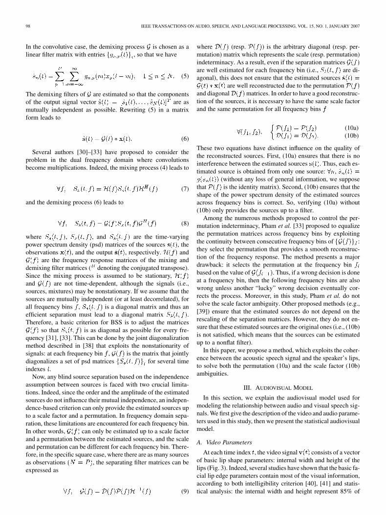
Fig. 8. Distortion (39) versus number of integration frames. Solid line: AV es-timation (36) and dashed-dot line: audio estimation (31).

For this purpose, the signal of interest [obtained bythe Fourier transform of ] is arbitrary multiplied by a scalefactor randomly chosen at each frequency bin.

To quantify the performance, we defined the distorsion as

(38)

In the specific case of this experiment, where there is no permu-tation, the distortion (38) no more depends on time and can beexpressed as

(39)

Fig. 8 shows the mean distortion versus the number of inte-gration frames for both audio (31) and audiovisual (36) estima-tions. Each simulation is repeated over 60 different logatoms.Fortunately, for both estimations, the distortion decreases whilethe number of integration frame increases. This is due to thefact that the variance of a particular section of speech can bedifferent of the variance of the model: the more numerous theintegration frames are, the more robust the estimation is. More-over, the AV estimation (36) is better than the audio one (31),justifying our idea that the video parameters can efficiently im-prove the estimation of the model variance corresponding of theparticular utterance of speech. Thus, for an arbitrary distortion,the number of integration frames is smaller with an AV estima-tion than with an audio one.

C. Permutation Results

To estimate the performance of our permutation cancellationalgorithm, we test permutation detection of blocks of consec-utive frequencies. As in the previous section, no mixing orseparation were performed. We simply artificially permutedsome blocks of consecutive frequencies between the twosources and obtained by the FFT of and

. Then, we applied our permutation cancellation algorithm

Fig. 9. Percentage of errors versus number of integration frames. Solid line:permutation of 250-Hz bandwidth blocks, dashed-dot line: permutation of100-Hz bandwidth blocks.

(Section IV-B) on these artificially modified signals. First,we test the permutation of 250-Hz bandwidth blocks (corre-sponding to five consecutive frequencies) for 1, 4, 8, 12, and16 permuted blocks. In this case, the smallest bandwidth of theblock used in our algorithm is equal to 250 Hz. Second, we testthe permutation of 100-Hz bandwidth blocks (corresponding totwo consecutive frequencies) for 1, 10, 20, 30, and 40 permutedblocks. In this case, the smallest bandwidth of the block usedin our algorithm is equal to 100 Hz.

We define the detection error as the sum of the unsolved per-mutations (actual permutations undetected by our algorithm)and the wrong permutations (bad decision of the algorithm).

For each experimental condition, the simulation is repeatedover 60 different logatoms which are randomly chosen but per-fectly known. Fig. 9 shows the mean percentage of detectionerror versus the number of integration frames for the two sim-ulation cases (100- and 250-Hz bandwidth blocks). This figurestresses the importance of integration for the criteria (22) and(24). Indeed, if the number of integration frames is too small, thepercentage of errors significantly increases while the computa-tional time decreases. Meanwhile, if the number of integrationframes increases, the number of errors decreases toward zerowhile the computational time increases. It can be noted that,for more than 40 integrated frames, the percentage of error issmaller than 5% for all tested conditions. Also, the mean resultsin the case of 250-Hz bandwidth block are better than the caseof 100-Hz bandwidth block. Thus, for an arbitrary percentageof errors, the resolution of the algorithm can be increased at theprice of a larger number of integration frames.

D. Separation Results

In the following, we consider the case of two sources[Fig. 10(a)] and two mixtures [Fig. 10(b)]. All mixing filters areartificial finite impulse response filters up to 320 lags: they fit asimplified acoustic model of a room impulse response (Fig. 11).Even if we plot the sources over four seconds, we only usedthe first 40 frames in order to estimate the permutation and the


Fig. 10. Sources, mixtures, and estimated sources.

Fig. 11. Mixing filters: impulse response of the four mixing filters.

scale factor. This value is coherent with the results obtained inthe previous sections.

An indicator of the separation performance is the perfor-mance index [33], defined as

(40)

where is the element of the global matrix filter. For a good separation, the index (40) should be close

to 0 (or infinity if a permutation has occurred).Fig. 12 plots and before and after ap-

plying our ambiguities detection. One can see that our methodcorrects all the permutations except one error: the performanceindex is always smaller than 1 except for one frequency. Thisis confirmed by the spectrum of the four impulse responses ofthe global filter (Fig. 13): for all the frequency bins(except for the error), (resp. ) is muchsmaller than (resp. ). This means thatthe global filter is close to a diagonal filter.

Fig. 12. Performance index r(f) [Eq. (40)] (dots) and its inverse (solid line)truncated at 1, before (upper panel) and after (lower panel) our ambiguities can-cellation versus the frequency.

Fig. 13. Global filter: spectrum of the four global filters estimated with ourambiguities cancellation.


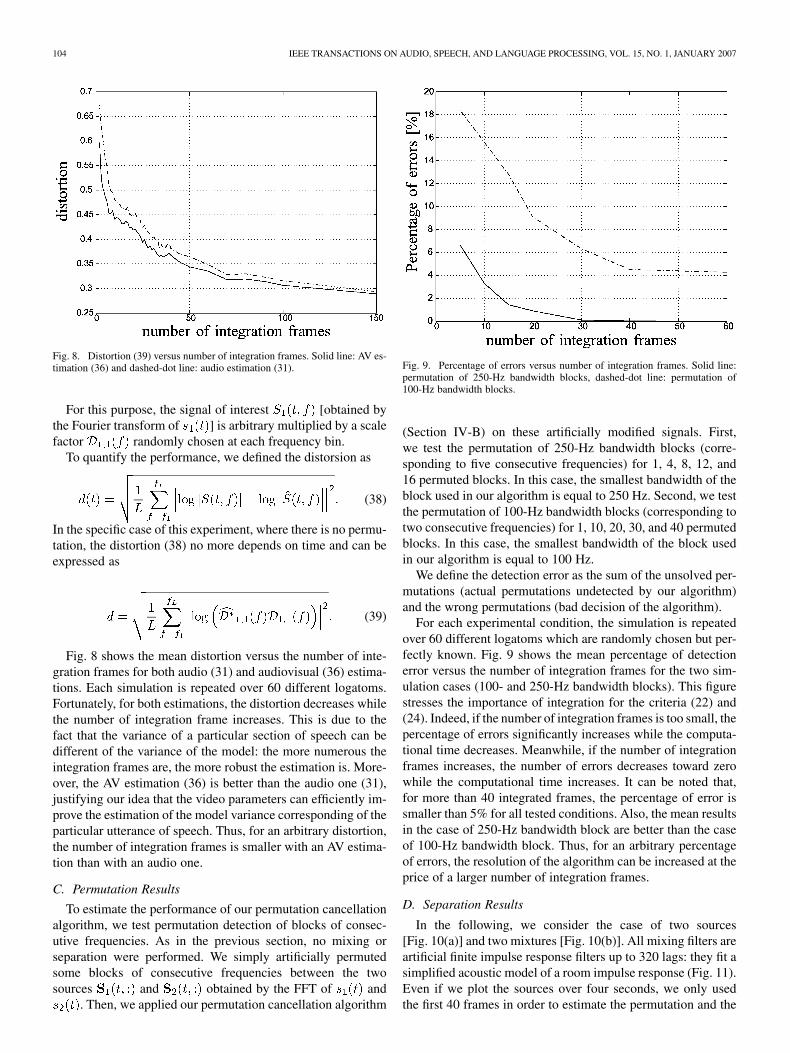
Fig. 14. Global filter without scale factor estimation.

Finally, Fig. 14 shows the spectrum of the global filter wherewe only made the permutation cancellation: we estimated thepermuted frequency bins with our ambiguities cancellation al-gorithm (Section IV-D) and then the global filter is estimatedby (i.e., without scale factor cancellation). Onecan see that is much closer to a constant with thescale factor cancellation (Fig. 13) than without scale factor can-cellation (Fig. 14). This provides a better estimation of the spec-trum shape of the estimated source of interest. Moreover, notethat and are left unchanged since ourcriteria only consider channel 1.

VI. CONCLUSION

The BSS problem of convolutive speech mixtures can be pro-cessed by using a pure audio technique like a joint diagonal-ization process in the time-frequency domain [30]–[33]. How-ever, this only provides a solution up to a permutation and ascale factor at each frequency bin. In this paper, we proposeda new statistical AV model expressing the complex relationshipbetween two basic lip video parameters and acoustic speech pa-rameters which consisted in the log-modulus of the coefficientsof the short-time Fourier transform. The series of experimentspresented in this paper, using our new AV model, confirm the in-terest of using AV processing to solve these ambiguities. How-ever, the method required integration over a large number offrames to obtain a good estimation of the permutations. Thus,our method is very efficient in order to estimate large blocks ofconsecutive permuted frequencies (20 to 40 frames are enoughin this case). However, over 100 frames are generally necessaryto find isolated permuted frequency. Note that our presentedmethod uses criteria which only consider one source of interest.If we extend the criteria to two sources of interest, the estimationof permutation is quite more efficient. Indeed, if the models oftwo distinct sources are known, then if a permutation is not de-tected by one of them, the other may find the permutation. In thispaper, we are not only interested in the permutation problem, but

Fig. 15. Probability density function of a Log–Rayleigh of parameter � = 1.

also in the scale factor: doing this, we improve both the permu-tation detection and the estimation of the sources.

It is already possible to assert that our AV method seemsuseful and original to estimate the ambiguities in the difficultand realistic problem of convolutive mixtures. Indeed, we usean additional video information, which is intrinsically robust toacoustic noise. A major strength of our method is that it can ex-tract a speech source from any kind of corrupting signals.

Finally, since the dimension of the parameters vector is large,a further step could be to search for other more efficient datarepresentations and/or associated algorithms. Of course, otherdevelopments are still necessary for a complete demonstrationof the efficiency of the proposed method: a first step could be todo experiments on a larger and more complex corpus, includingcontinuous speech material and multispeaker AV models. Weare currently working on this topic.

APPENDIX ILOG–RAYLEIGH DISTRIBUTION

In this appendix, we briefly recall the definition of thelog–Rayleigh distribution (for more details refer to [36]).

Definition 1: Let denote a Log–Rayleigh random variablewith localization parameter . The prob-ability density function of this variable is given by

(41)

This distribution is plotted in Fig. 15.In the multidimensional case, for sake of simplicity, we note

the log–Rayleigh distribution where the parameteris the diagonal matrix which is the

product of the monodimensional Log–Rayleigh distribution

(42)

APPENDIX IILEARNING THE AUDIOVISUAL MODEL

In this appendix, we use the EM algorithm [50] in a penal-ized version [48], [49] to obtain the update equations for the au-diovisual model (13). The EM algorithm is a recursive method


to estimate the parameter setthanks to the maximum likelihood. There are two stages.

1) Expectation (E): calculation of the a posteriori probability

where refers to the parameters at the th iteration.2) Maximization (M): update of the parameters

• weight

• video parameters

and for equal to or :

where and are the penalized parameters [48],• the audio parameters, for all

REFERENCES

[1] L. E. Bernstein and C. Benoît, “For speech perception by humans ormachines, three senses are better than one,” in Proc. Int. Conf. SpokenLang. Process. (ICSLP), 1996, pp. 1477–1480.

[2] W. Sumby and I. Pollack, “Visual contribution to speech intelligibilityin noise,” J. Acoust. Soc. Amer., vol. 26, pp. 212–215, 1954.

[3] Q. Summerfield, “Some preliminaries to a comprehensive account ofaudio-visual speech perception,” in Hearing by Eye: The Psychology ofLipreading, B. Dodd and R. Campbell, Eds. Mahwah, NJ: LawrenceErlbaum, 1987, pp. 3–51.

[4] J. Robert-Ribes, J.-L. Schwartz, T. Lallouache, and P. Escudier,“Complementarity and synergy in bimodal speech: Auditory, visual,and audio-visual identification of French oral vowels in noise,” J.Acoust. Soc. Amer., vol. 103, no. 6, pp. 3677–3689, 1998.

[5] E. D. Petajan, “Automatic lipreading to enhance speech recognition,”Ph.D. dissertation, Univ. Illinois, Urbana, 1984.

[6] G. Potamianos, C. Neti, G. Gravier, A. Garg, and A. W. Senior, “Recentadvances in the automatic recognition of audio-visual speech,” Proc.IEEE, vol. 91, no. 9, pp. 1306–1326, Sep. 2003.

[7] K. Grant and P. Seitz, “The use of visible speech cues for improvingauditory detection of spoken sentences,” J. Acoust. Soc. Amer., vol.108, pp. 1197–1208, 2000.

[8] J. Kim and D. Chris, “Investigating the audio-visual speech detectionadvantage,” Speech Commun., vol. 44, no. 1–4, pp. 19–30, 2004.

[9] L. E. Bernstein, E. T. J. Auer, and S. Takayanagi, “Auditory speechdetection in noise enhanced by lipreading,” Speech Commun., vol. 44,no. 1–4, pp. 5–18, 2004.

[10] J.-L. Schwartz, F. Berthommier, and C. Savariaux, “Audio-visual sceneanalysis; evidence for a “very-early” integration process in audio-visualspeech perception,” in Proc. Int. Conf. Spoken Lang. Process. (ICSLP),2002, pp. 1937–1940.

[11] L. Girin, J.-L. Schwartz, and G. Feng, “Audio-visual enhancement ofspeech in noise,” J. Acoust. Soc. Amer., vol. 109, no. 6, pp. 3007–3020,Jun. 2001.

[12] S. Deligne, G. Potamianos, and C. Neti, “Audio-visual speechenhancement with AVCDCN (AudioVisual Codebook DependentCepstral Normalization),” in Proc. Int. Conf. Spoken Lang. Process.(ICSLP), 2002, pp. 1449–1452.

[13] R. Goecke, G. Potamianos, and C. Neti, “Noisy audio feature enhance-ment using audio-visual speech data,” in Proc. IEEE Int. Conf. Acous-tics, Speech, Signal Process. (ICASSP), Orlando, FL, May 2002, pp.2025–2028.

[14] L. Girin, A. Allard, and J.-L. Schwartz, “Speech signals separation: Anew approach exploiting the coherence of audio and visual speech,”in IEEE Int. Workshop Multimedia Signal Process. (MMSP), Cannes,France, 2001.

[15] D. Sodoyer, J.-L. Schwartz, L. Girin, J. Klinkisch, and C. Jutten, “Sep-aration of audio-visual speech sources: a new approach exploiting theaudiovisual coherence of speech stimuli,” EURASIP J. Appl. SignalProcess., vol. 2002, no. 11, pp. 1165–1173, 2002.

[16] D. Sodoyer, L. Girin, C. Jutten, and J.-L. Schwartz, “Developing anaudio-visual speech source separation algorithm,” Speech Commun.,vol. 44, no. 1–4, pp. 113–125, Oct. 2004.

[17] J.-F. Cardoso, “Blind signal separation: statistical principles,” Proc.IEEE, vol. 86, no. 10, pp. 2009–2025, Oct. 1998.

[18] C. Jutten and A. Taleb, “Source separation: from dusk till dawn,” inProc. Int. Conf. Independent Compon. Anal. Blind Source Separation(ICA), Helsinki, Finland, Jun. 2000, pp. 15–26.

[19] A. Hyvärinen, J. Karhunen, and E. Oja, Independent Component Anal-ysis. New York: Wiley, 2001.

[20] P. Comon, “Independent component analysis, a new concept?,” SignalProcess., vol. 36, no. 3, pp. 287–314, Apr. 1994.

[21] J. Hérault, C. Jutten, and B. Ans, “Détection de grandeurs prim-itives dans un message composite par une architecture de calculneuromimétrique en apprentissage non supervisé,” in Proc. GRETSI,Nice, France, May 1985, vol. 2, pp. 1017–1020.

[22] C. Jutten and J. Hérault, “Blind separation of sources. Part I: An adap-tive algorithm based on a neuromimetic architecture,” Signal Process.,vol. 24, no. 1, pp. 1–10, Jul. 1991.

[23] J.-F. Cardoso and A. Souloumiac, “Blind beamforming for nonGaussian signals,” Proc. Inst. Elect. Eng. F, vol. 140, no. 6, pp.362–370, Dec. 1993.

[24] A. Hyvarinen, “Fast and robust fixed-point algorithms for independentcomponent analysis,” IEEE Trans. Neural Netw., vol. 10, no. 3, pp.626–634, May 1999.

[25] A. Bell and T. Sejnowski, “An information-maximization approach toblind source separation and blind deconvolution,” Neural Comput., vol.7, pp. 1129–1159, 1995.

[26] L. De Lathauwer, D. Callaerts, B. De Moor, and J. Vandewalle, “Fetalelectrocardiogram extraction by source subspace separation,” in Proc.IEEE Workshop HOS, Girona, Spain, Jun. 12–14, 1995, pp. 134–138.

[27] V. Zarzoso and A. K. Nandi, “Noninvasive fetal electrocardiogram ex-traction: Blind source separation versus adaptative noise cancellation,”IEEE Trans. Biomed. Eng., vol. 48, no. 1, pp. 12–18, Jan. 2001.

[28] R. Dansereau, “Co-channel audiovisual speech separation using spec-tral matching constraints,” in Proc. IEEE Int. Conf. Acoust., Speech,Signal Process. (ICASSP), Montréal, QC, Canada, 2004.

[29] S. Rajaram, A. V. Nefian, and T. S. Huang, “Bayesian separationof audio-visual speech sources,” in Proc. IEEE Int. Conf. Acoustics,Speech, and Signal Processing (ICASSP), Montréal, Canada, 2004,pp. 645–648.

[30] V. Capdevielle, C. Servière, and J.-L. Lacoume, “Blind separation ofwide-band sources in the frequency domain,” in Proc. IEEE Int. Conf.Acoust., Speech, Signal Process. (ICASSP), Detroit, MI, May 1995, pp.2080–2083.


[31] L. Para and C. Spence, “Convolutive blind separation of non stationarysources,” IEEE Trans. Speech Audio Process., vol. 8, no. 3, pp.320–327, May 2000.

[32] A. Dapena, M. F. Bugallo, and L. Castedo, “Separation of convolutivemixtures of temporally-white signals: A novel frequency-domain ap-proach,” in Proc. Int. Conf. Independent Compon. Anal. Blind SourceSeparation (ICA), San Diego, CA, Dec. 2001, pp. 315–320.

[33] D.-T. Pham, C. Servière, and H. Boumaraf, “Blind separation of con-volutive audio mixtures using nonstationary,” in Proc. Int. Conf. Inde-pendent Compon. Anal. Blind Source Separation (ICA), Nara, Japan,Apr. 2003, pp. 981–986.

[34] B. Rivet, L. Girin, C. Jutten, and J.-L. Schwartz, “Using audiovisualspeech processing to improve the robustness of the separation of con-volutive speech mixtures,” in IEEE Int. Workshop Multimedia SignalProcess. (MMSP), Sienna, Italy, Oct. 2004, pp. 47–50.

[35] B. Rivet, L. Girin, and C. Jutten, “Solving the indeterminations of blindsource separation of convolutive speech mixtures,” in Proc. IEEE Int.Conf. Acoust., Speech, Signal Process. (ICASSP), Philadelphia, PA,Mar. 2005, pp. 533–536.

[36] ——, “Log-Rayleigh distribution: A simple and efficient statistical rep-resentation of log-spectral coefficients,” IEEE Trans. Audio, Speech,Lang. Process., 2006, submitted for publication.

[37] H.-L. Nguyen-Thi and C. Jutten, “Blind source separation for convo-lutive mixtures,” Signal Process., vol. 45, pp. 209–229, 1995.

[38] D.-T. Pham, “Joint approximate diagonalization of positive definitematrices,” SIAM J. Matrix Anal. Appl., vol. 22, no. 4, pp. 1136–1152,2001.

[39] N. Murata, S. Ikeda, and A. Ziehe, “An approach to blind source sep-aration based on temporal structure of speech signals,” Neurocomput.,vol. 41, no. 1–4, pp. 1–24, Oct. 2001.

[40] B. Le Goff, T. Guiard-Marigny, and C. Benoît, “Read my lips. . . andmy jaw! How intelligible are the components of a speaker’s face?,” inProc. Euro. Conf. Speech Communication Technology, Madrid, Spain,1995, pp. 291–294.

[41] ——, “Analysis-synthesis and intelligibility of a talking face,” inProgress in Speech SynthesisJ. Van Santen, R. Sproat, J. Olive, and J.Hirschberg, Eds. New York: Springer-Verlag, 1996, pp. 235–244.

[42] F. Elisei, M. Odisio, G. Bailly, and P. Badin, “Creating and controllingvideo-realistic talking heads,” in Proc. Audio-Visual Speech ProcessingWorkshop (AVSP), Aalborg, Denmark, 2001, pp. 90–97.

[43] T. Lallouache, “Un poste visage-parole. Acquisition et traitement descontours labiaux,” in Proc. Journées d’Etude sur la Parole (JEP) (inFrench), Montréal, QC, Canada, 1990, pp. 282–286.

[44] B. Picinbono, “Second-order complex random vectors and normaldistributions,” IEEE Trans. Signal Process., vol. 44, no. 10, pp.2637–2640, Oct. 1996.

[45] F. D. Neeser and J. L. Massey, “Proper complex random processes withapplications to information theory,” IEEE Trans. Inf. Theory, vol. 39,no. 4, pp. 1293–1302, Jul. 1993.

[46] L. Benaroya, “Séparation de plusieurs sources sonores avec un seulmicrophone,” Ph.D. dissertation, Traitement du signal, Univ. Rennes1, Rennes, France, Jun. 2003.

[47] H. Yehia, P. Rubin, and E. Vatikiotis-Bateson, “Quantitative associa-tion of vocal-tract and facial behavior,” Speech Commun., vol. 26, no.1, pp. 23–43, 1998.

[48] D. Ormoneit and V. Tresp, “Averaging, maximum penalized likeli-hood and Bayesian estimation for improving Gaussian mixture proba-bility density estimates,” IEEE Trans. Neural Netw., vol. 9, no. 4, pp.639–650, Jul. 1998.

[49] H. Snoussi and A. Mohammad-Djafari, “Penalized maximum likeli-hood for multivariate Gaussian mixture,” in Proc. Bayesian Inferenceand Maximum Entropy Methods, R. L. Fry, Ed. MaxEnt Workshops,Aug. 2001, pp. 36–46.

[50] A. P. Dempster, N. M. Laird, and D. B. Rubin, “Maximum-likelihoodfrom incomplete data via the EM algorithm,” J. R. Statist. Soc. Ser. B.,vol. 39, pp. 1–38, 1977.

Bertrand Rivet graduated from the École NormaleSupérieure de Cachan, Cachan, France, and receivedthe Agrégation de Physique Appliquée and theMaster’s degree from the University of Paris-XI,Orsay, France, in 2002 and 2003, respectively. Heis currently pursuing the Ph.D. degree in signalprocessing at the Institut de la CommunicationParlée (Speech Communication Laboratory) and atthe Laboratoire des Images et des Signaux (Imagesand Signals Laboratory), Grenoble, France.

His research concerns audiovisual speech andblind source separation.

Laurent Girin received the M.Sc. and Ph.D. degreesin signal processing from the Institut NationalPolytechnique de Grenoble, Grenoble, France, in1994 and 1997, respectively.

In 1997, he joined the Ecole Nationale d’Elec-tronique et de Radioélectricité de Grenoble, wherehe is currently an Associate Professor in electricalengineering and signal processing. His researchactivity takes place in the Institut de la Communi-cation Parlée (Speech Communication Laboratory)in Grenoble. His current research interests concern

audiovisual speech processing with application to speech coding, speechenhancement, and audio/speech source separation, and also acoustic speechanalysis, modeling and synthesis.

Christian Jutten received the Ph.D. and the Doc-teur ès Sciences degrees from the Institut NationalPolytechnique of Grenoble, Grenoble, France, in1981 and 1987, respectively.

He was an Associate Professor with the EcoleNationale Supérieure d’Electronique et de Ra-dioélectricité, Grenoble, from 1982 to 1989. Hewas a Visiting Professor with the Swiss FederalPolytechnic Institute, Lausanne, Switzerland, in1989, before becoming a Full Professor with theUniversité Joseph Fourier, Grenoble, more precisely

in Polytech’Grenoble Institute. He is currently an Associate Director of theImages and Signals Laboratory (100 people). For 25 years, his research inter-ests have been in blind source separation, independent component analysis,and learning in neural networks, including theoretical aspects (separability,source separation in nonlinear mixtures), applications in signal processing(biomedical, seismic, speech), and data analysis. He is author or coauthorof more than 40 papers in international journals, 16 invited paper, and 100communications in international conferences.

Prof. Jutten was an Associate Editor of the IEEE TRANSACTIONS ON CIRCUITS

AND SYSTEMS (1994–19 95) and coorganizer the First International Conferenceon Blind Signal Separation and Independent Component Analysis (Aussois,France, January 1999). He is a Reviewer of main international journals (IEEETRANSACTIONS ON SIGNAL PROCESSING, IEEE SIGNAL PROCESSING LETTERS,IEEE TRANSACTIONS ON NEURAL NETWORKS, Signal Processing, Neural Com-putation, Neurocomputing, etc.) and conferences in signal processing and neuralnetworks (ICASSP, ISCASS, EUSIPCO, IJCNN, ICA, ESANN, IWANN, etc.).

96 ieee transactions on audio, speech, and language processing

Documents