9 hypothesistests · 3 componentsofahypothesistest 1. formulatethehypothesistobetested. 2....

9 Hypothesis Tests

(Ch 9.1-9.3, 9.5-9.9)

2

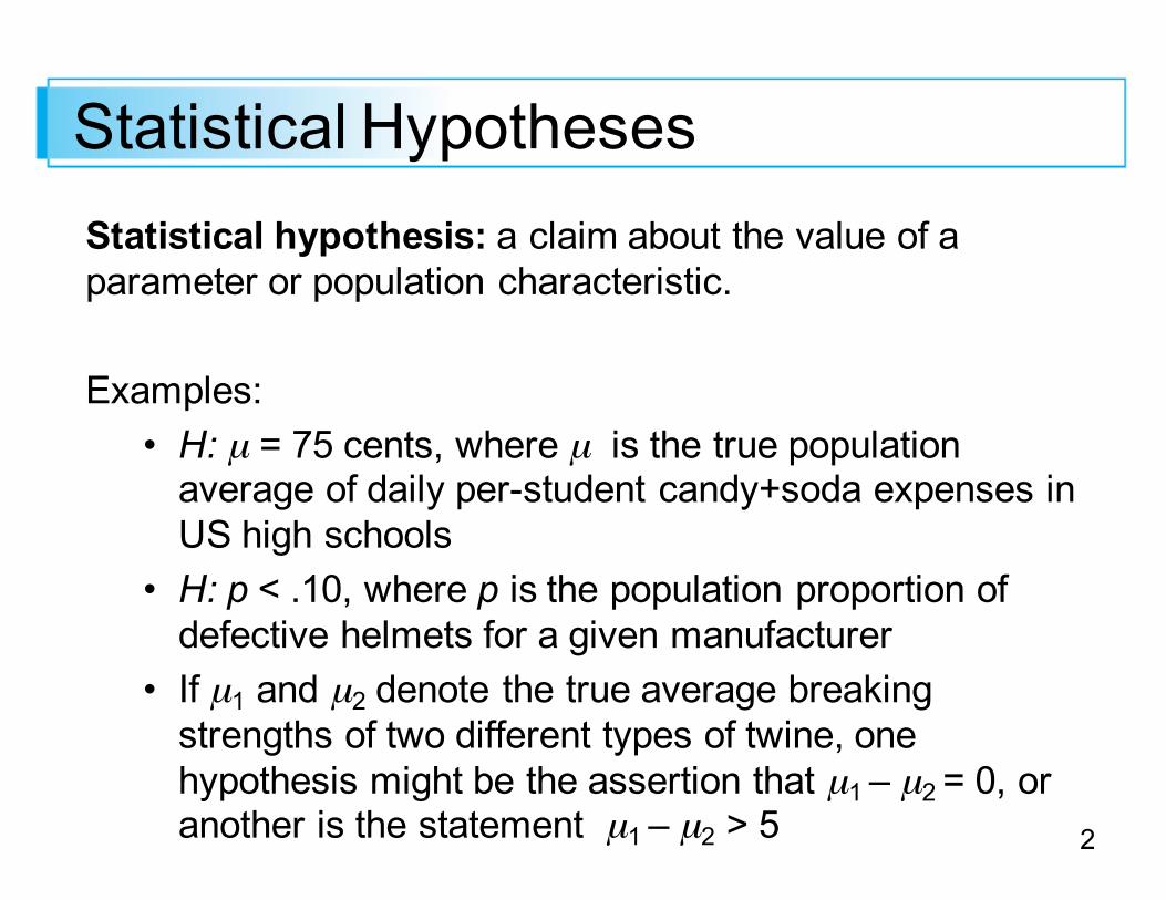
Statistical HypothesesStatistical hypothesis: a claim about the value of a parameter or population characteristic.

Examples: • H: µ = 75 cents, where µ is the true population average of daily per-student candy+soda expenses in US high schools

• H: p < .10, where p is the population proportion of defective helmets for a given manufacturer

• If µ1 and µ2 denote the true average breaking strengths of two different types of twine, one hypothesis might be the assertion that µ1 – µ2 = 0, or another is the statement µ1 – µ2 > 5

3

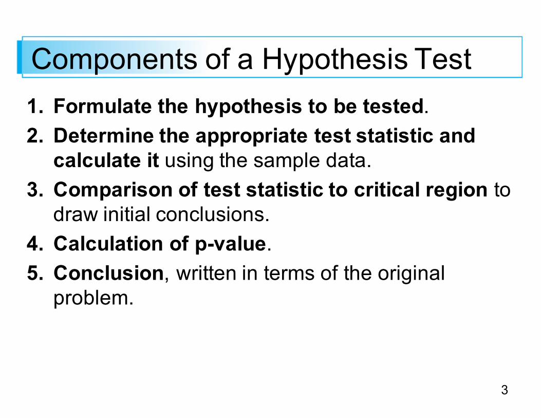
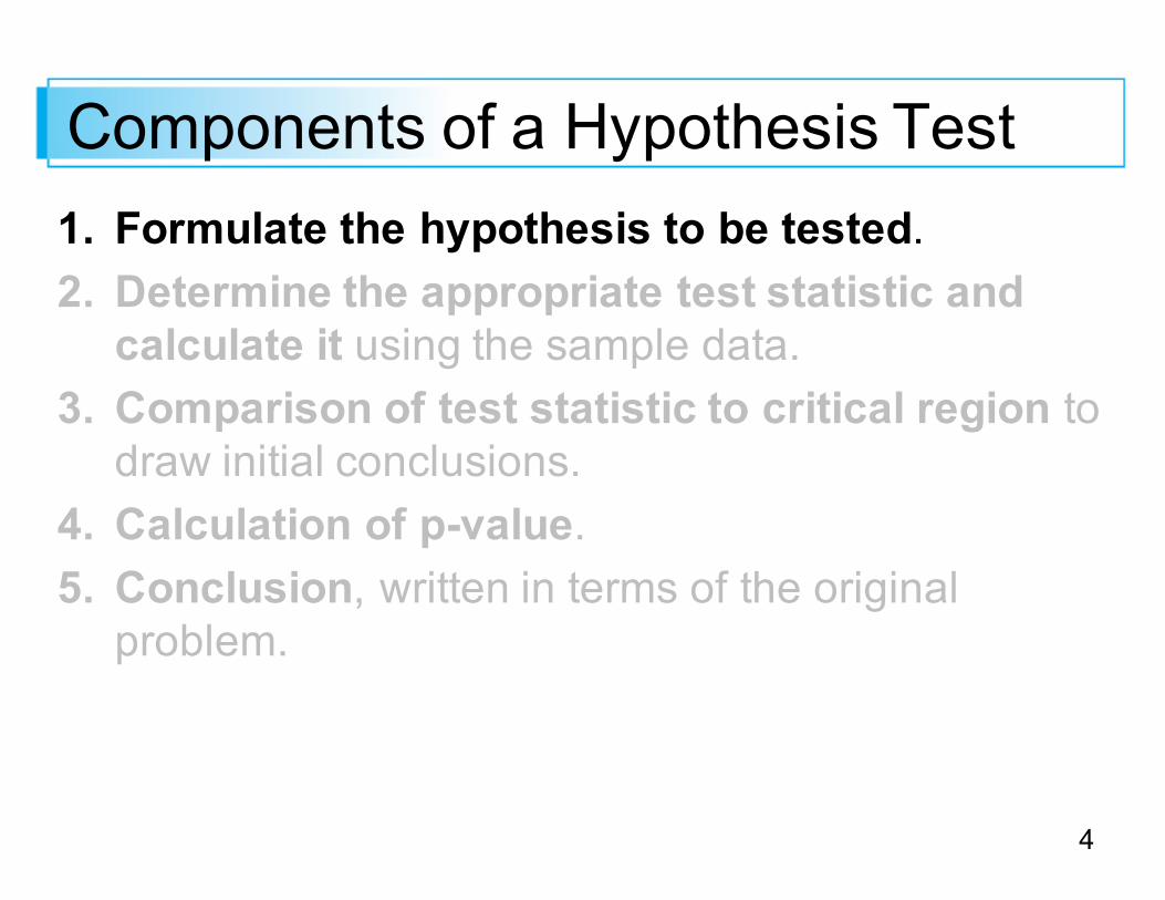
Components of a Hypothesis Test1. Formulate the hypothesis to be tested.2. Determine the appropriate test statistic and calculate it using the sample data.

3. Comparison of test statistic to critical region to draw initial conclusions.

4. Calculation of p-value.5. Conclusion, written in terms of the original problem.

4




5

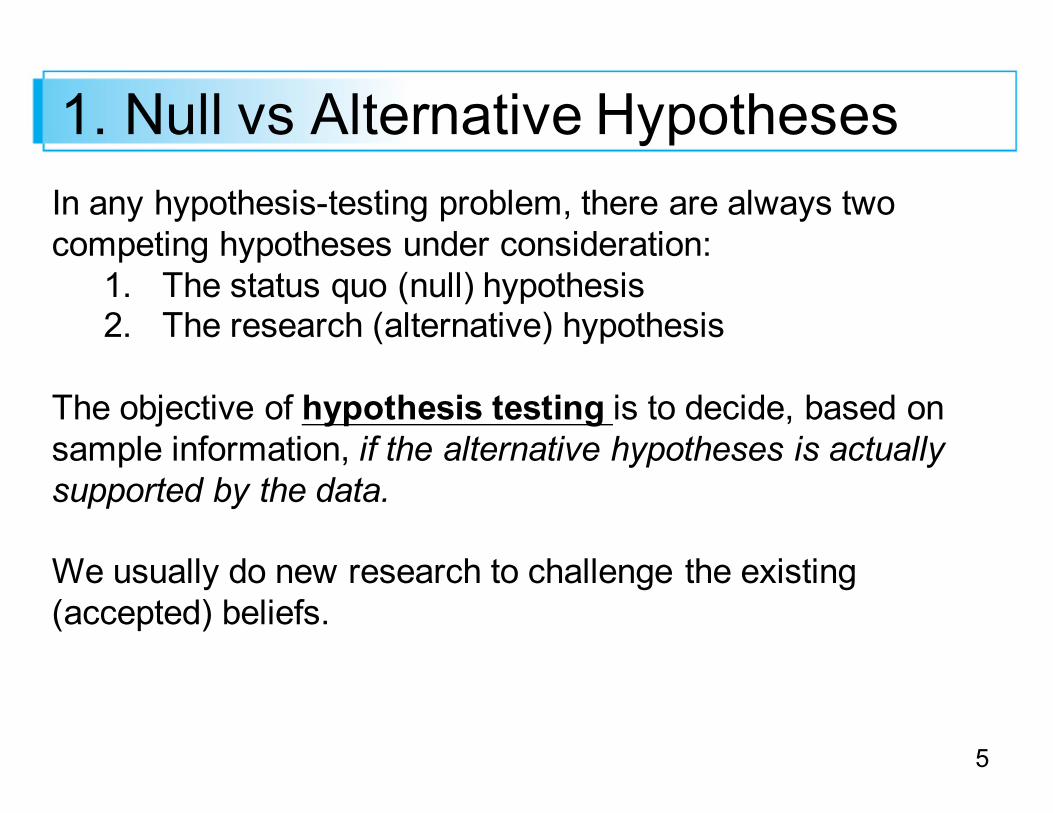
1. Null vs Alternative HypothesesIn any hypothesis-testing problem, there are always two competing hypotheses under consideration:1. The status quo (null) hypothesis 2. The research (alternative) hypothesis

The objective of hypothesis testing is to decide, based on sample information, if the alternative hypotheses is actually supported by the data.

We usually do new research to challenge the existing (accepted) beliefs.

6

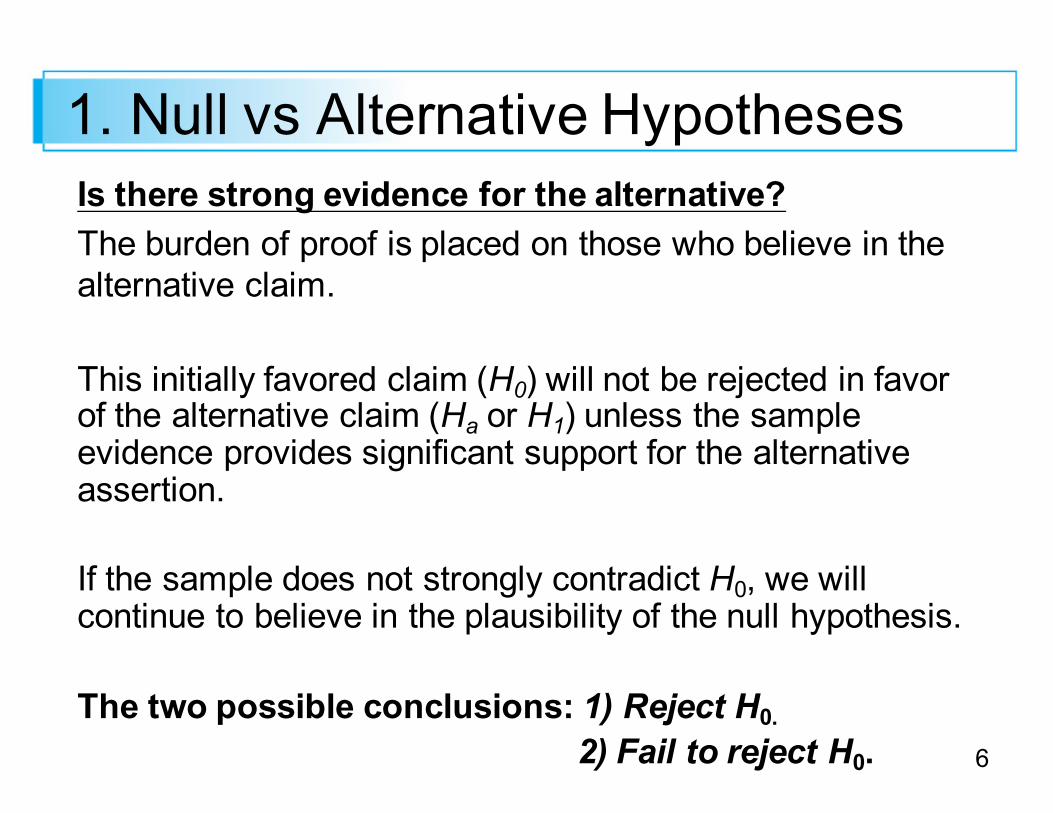
1. Null vs Alternative HypothesesIs there strong evidence for the alternative? The burden of proof is placed on those who believe in the alternative claim.

This initially favored claim (H0) will not be rejected in favor of the alternative claim (Ha or H1) unless the sample evidence provides significant support for the alternative assertion.

If the sample does not strongly contradict H0, we will continue to believe in the plausibility of the null hypothesis.

The two possible conclusions: 1) Reject H0.2) Fail to reject H0.

7

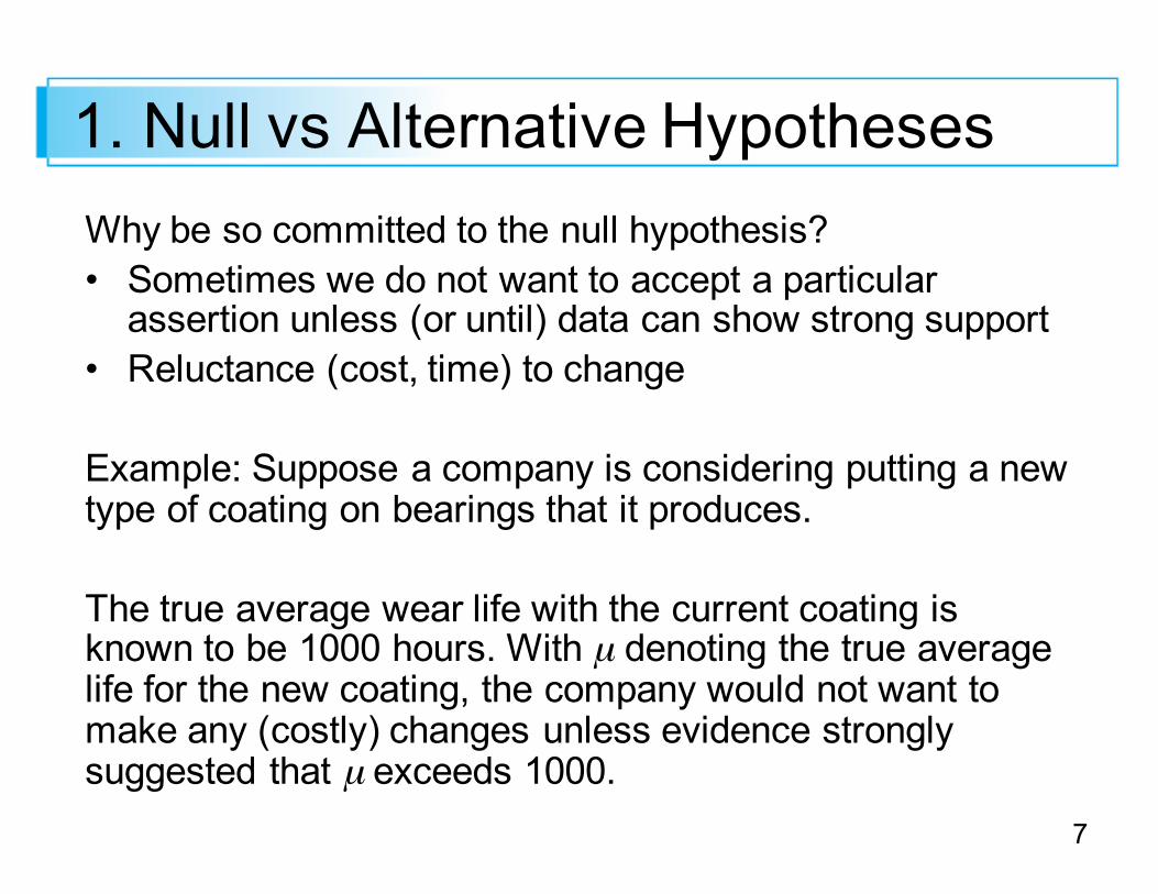
1. Null vs Alternative HypothesesWhy be so committed to the null hypothesis? • Sometimes we do not want to accept a particular assertion unless (or until) data can show strong support

• Reluctance (cost, time) to change

Example: Suppose a company is considering putting a new type of coating on bearings that it produces.

The true average wear life with the current coating is known to be 1000 hours. With µ denoting the true average life for the new coating, the company would not want to make any (costly) changes unless evidence strongly suggested that µ exceeds 1000.

8

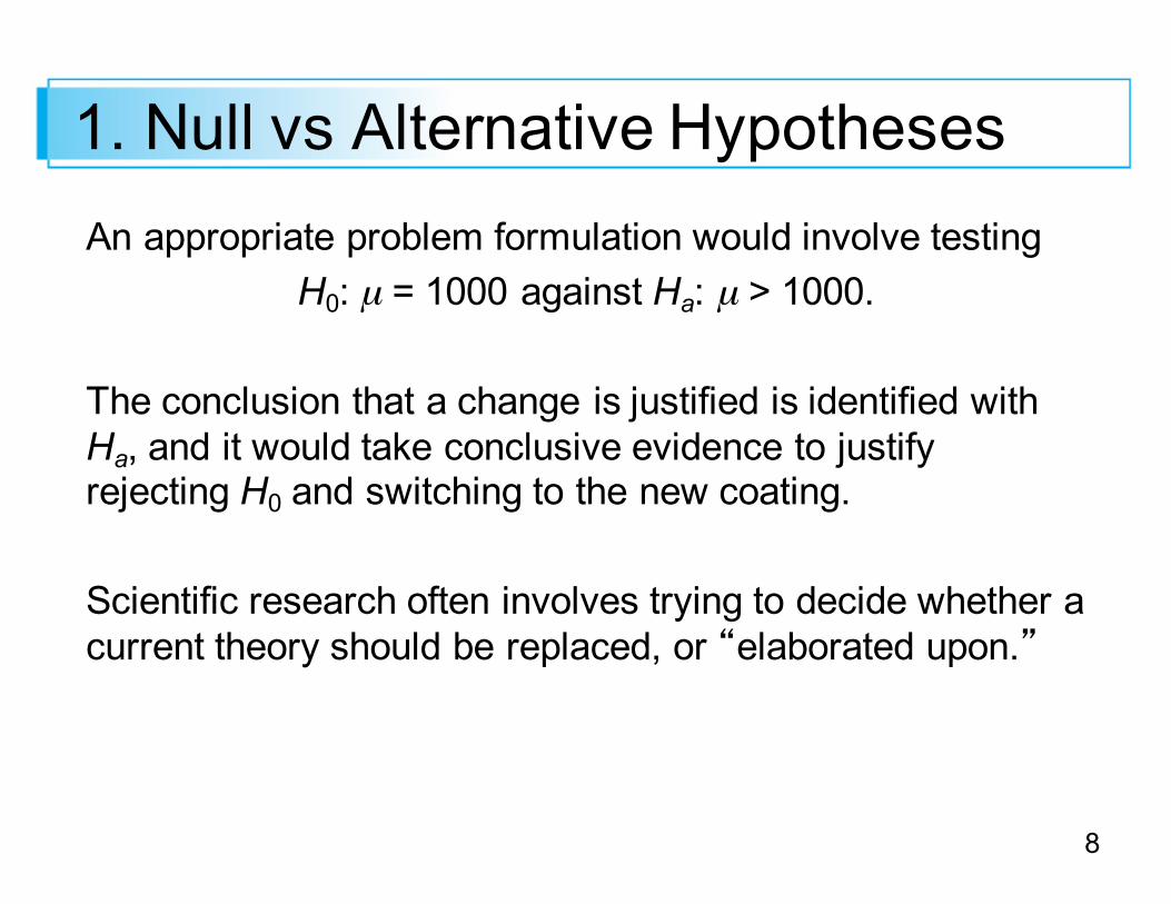
1. Null vs Alternative HypothesesAn appropriate problem formulation would involve testing

H0: µ = 1000 against Ha: µ > 1000.

The conclusion that a change is justified is identified with Ha, and it would take conclusive evidence to justify rejecting H0 and switching to the new coating.

Scientific research often involves trying to decide whether a current theory should be replaced, or “elaborated upon.”

9

1. Null vs Alternative HypothesesThe alternative to the null hypothesis H0: θ = θ0 will look like one of the following three assertions:

1. Ha: θ ≠ θ02. Ha: θ > θ0 (in which case the null hypothesis is θ ≤ θ0)3. Ha: θ < θ0 (in which case the null hypothesis is θ ≥ θ0)

• The equality sign is always with the null hypothesis.• The alternate hypothesis is the claim for which we are seeking statistical proof.

10




11

2. Test StatisticsA test statistic is a rule, based on sample data, for deciding whether to reject H0.

The test statistic is a function of the sample data that will be used to make a decision about whether the null hypothesis should be rejected or not.

12

2. Test StatisticsExample: Company A produces circuit boards, but 10% of them are defective. Company B claims that they produce fewer defective circuit boards.

H0: p = .10 versus Ha: p < .10

Our data is a random sample of n = 200 boards from company B.

What test procedure (or rule) could we devise to decide if the null hypothesis should be rejected?

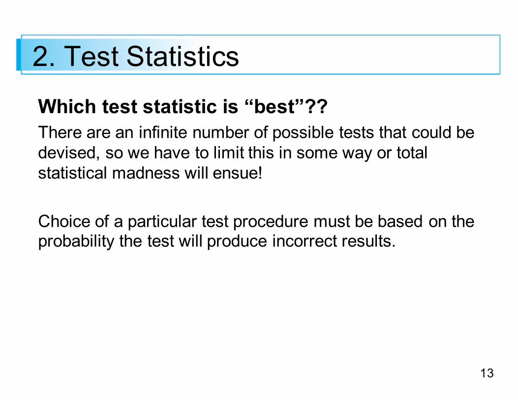
13

2. Test StatisticsWhich test statistic is “best”??There are an infinite number of possible tests that could be devised, so we have to limit this in some way or total statistical madness will ensue!

Choice of a particular test procedure must be based on the probability the test will produce incorrect results.

14

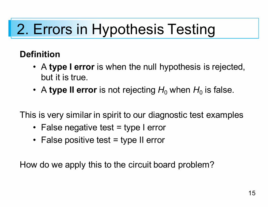
2. Errors in Hypothesis TestingDefinition • A type I error is when the null hypothesis is rejected, but it is true.

• A type II error is not rejecting H0 when H0 is false.

This is very similar in spirit to our diagnostic test examples• False negative test = type I error• False positive test = type II error

15

2. Errors in Hypothesis TestingDefinition • A type I error is when the null hypothesis is rejected, but it is true.

• A type II error is not rejecting H0 when H0 is false.

This is very similar in spirit to our diagnostic test examples• False negative test = type I error• False positive test = type II error

How do we apply this to the circuit board problem?

16

2. Type I errorsUsually: Specify the largest value of α that can be tolerated, and then find a rejection region with that α.

The resulting value of α is often referred to as the significance level of the test.

Traditional levels of significance are .10, .05, and .01, though the level in any particular problem will depend on the seriousness of a type I error—

The more serious the type I error, the smaller the significance level should be.

17

2. Errors in Hypothesis TestingWe can also obtain a smaller value of α -- the probability that the null will be incorrectly rejected – by decreasing the size of the rejection region.

However, this results in a larger value of β for all parameter values consistent with Ha.

No rejection region that will simultaneously make both αand all β’s small. A region must be chosen to strike a compromise between α and β.

18

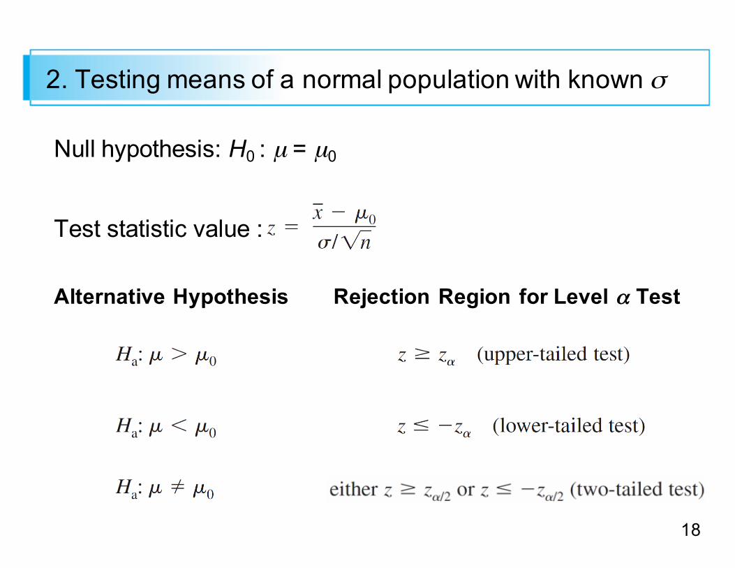
2. Testing means of a normal population with known σ

Null hypothesis: H0 : µ = µ0

Test statistic value :

Alternative Hypothesis Rejection Region for Level α Test

19




20

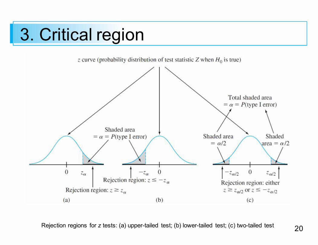
3. Critical region

Rejection regions for z tests: (a) upper-tailed test;; (b) lower-tailed test;; (c) two-tailed test

21

ExampleAn inventor has developed a new, energy-efficient lawn mower engine. He claims that the engine will run continuously for more than 5 hours (300 minutes) on a single gallon of regular gasoline. (The leading brand lawnmower engine runs for 300 minutes on 1 gallon of gasoline.)

From his stock of engines, the inventor selects a simple random sample of 50 engines for testing. The engines run for an average of 305 minutes. The true standard deviation σ is known and is equal to 30 minutes, and the run times of the engines are normally distributed.

Test hypothesis that the mean run time is more than 300 minutes. Use a 0.05 level of significance.

22

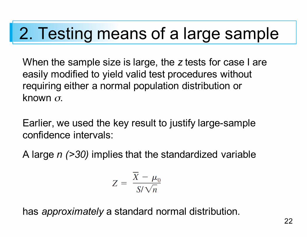
2. Testing means of a large sampleWhen the sample size is large, the z tests for case I are easily modified to yield valid test procedures without requiring either a normal population distribution or known σ.

Earlier, we used the key result to justify large-sample confidence intervals:

A large n (>30) implies that the standardized variable

has approximately a standard normal distribution.

23

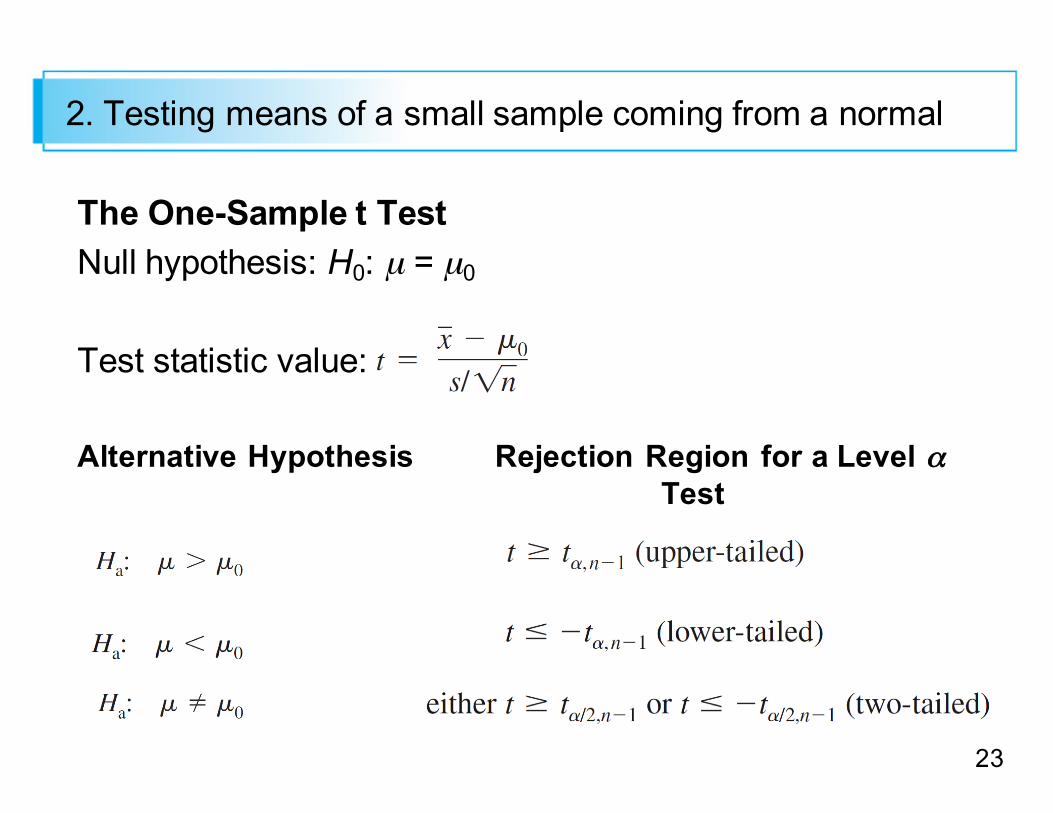
2. Testing means of a small sample coming from a normal

The One-Sample t TestNull hypothesis: H0: µ = µ0

Test statistic value:

Alternative Hypothesis Rejection Region for a Level αTest

24

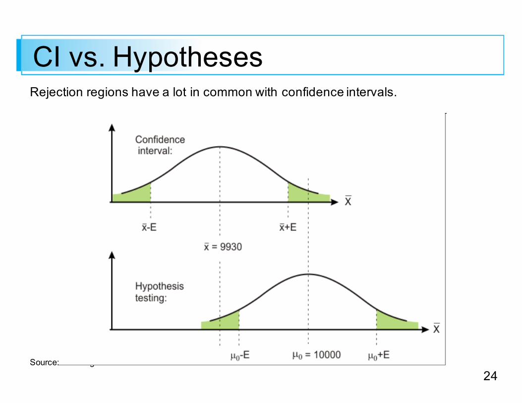
CI vs. HypothesesRejection regions have a lot in common with confidence intervals.

Source: shex.org

25

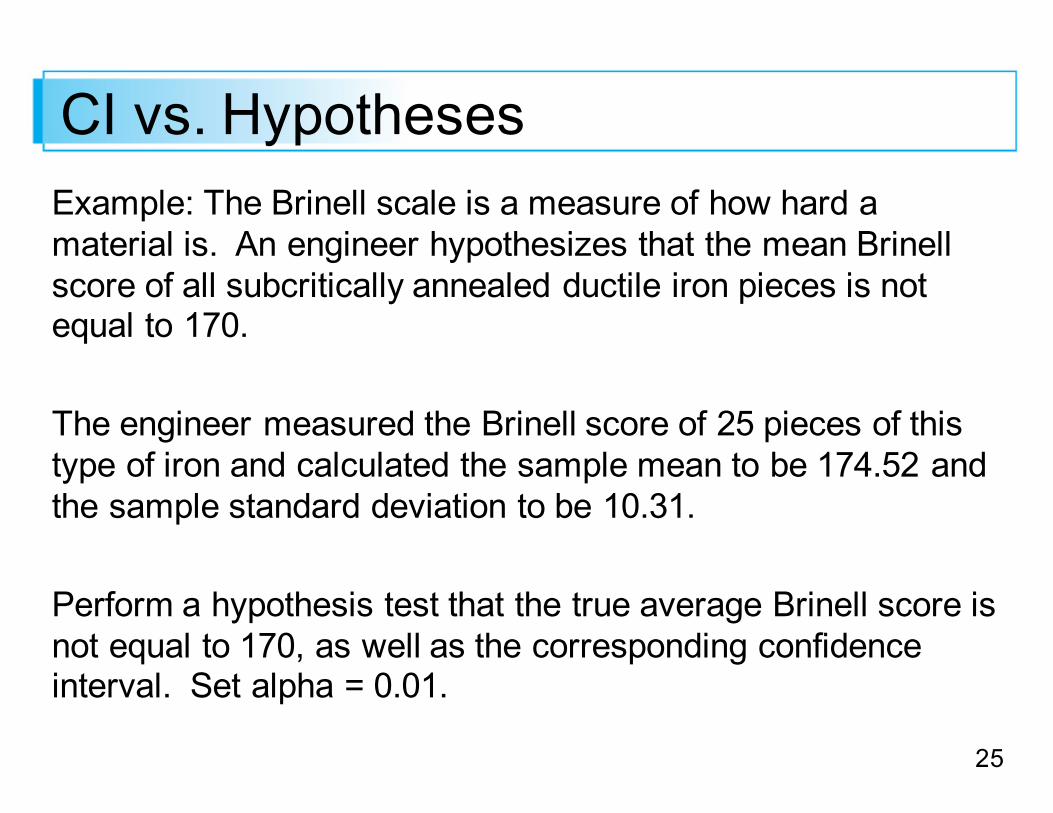
CI vs. HypothesesExample: The Brinell scale is a measure of how hard a material is. An engineer hypothesizes that the mean Brinellscore of all subcritically annealed ductile iron pieces is not equal to 170.

The engineer measured the Brinell score of 25 pieces of this type of iron and calculated the sample mean to be 174.52 and the sample standard deviation to be 10.31.

Perform a hypothesis test that the true average Brinell score is not equal to 170, as well as the corresponding confidence interval. Set alpha = 0.01.

26




27

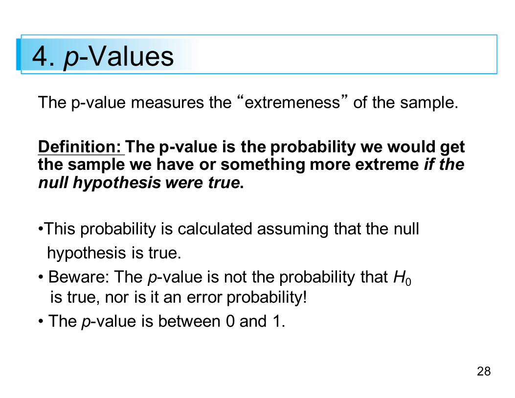
4. p-ValuesThe p-value measures the “extremeness” of the sample.

Definition: The p-value is the probability we would get the sample we have or something more extreme if the null hypothesis were true.

So, the smaller the P-value, the more evidence there is in the sample data against the null hypothesis and for the alternative hypothesis.

So what constitutes “sufficiently small” and “extreme enough” to make a decision about the null hypothesis?

28

4. p-ValuesThe p-value measures the “extremeness” of the sample.

Definition: The p-value is the probability we would get the sample we have or something more extreme if the null hypothesis were true.

•This probability is calculated assuming that the nullhypothesis is true.• Beware: The p-value is not the probability that H0 is true, nor is it an error probability!• The p-value is between 0 and 1.

29

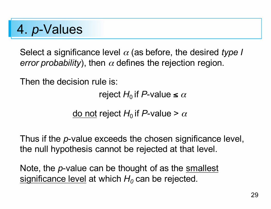
4. p-ValuesSelect a significance level α (as before, the desired type I error probability), then α defines the rejection region.

Then the decision rule is:reject H0 if P-value ≤ α

do not reject H0 if P-value > α

Thus if the p-value exceeds the chosen significance level, the null hypothesis cannot be rejected at that level.

Note, the p-value can be thought of as the smallest significance level at which H0 can be rejected.

30

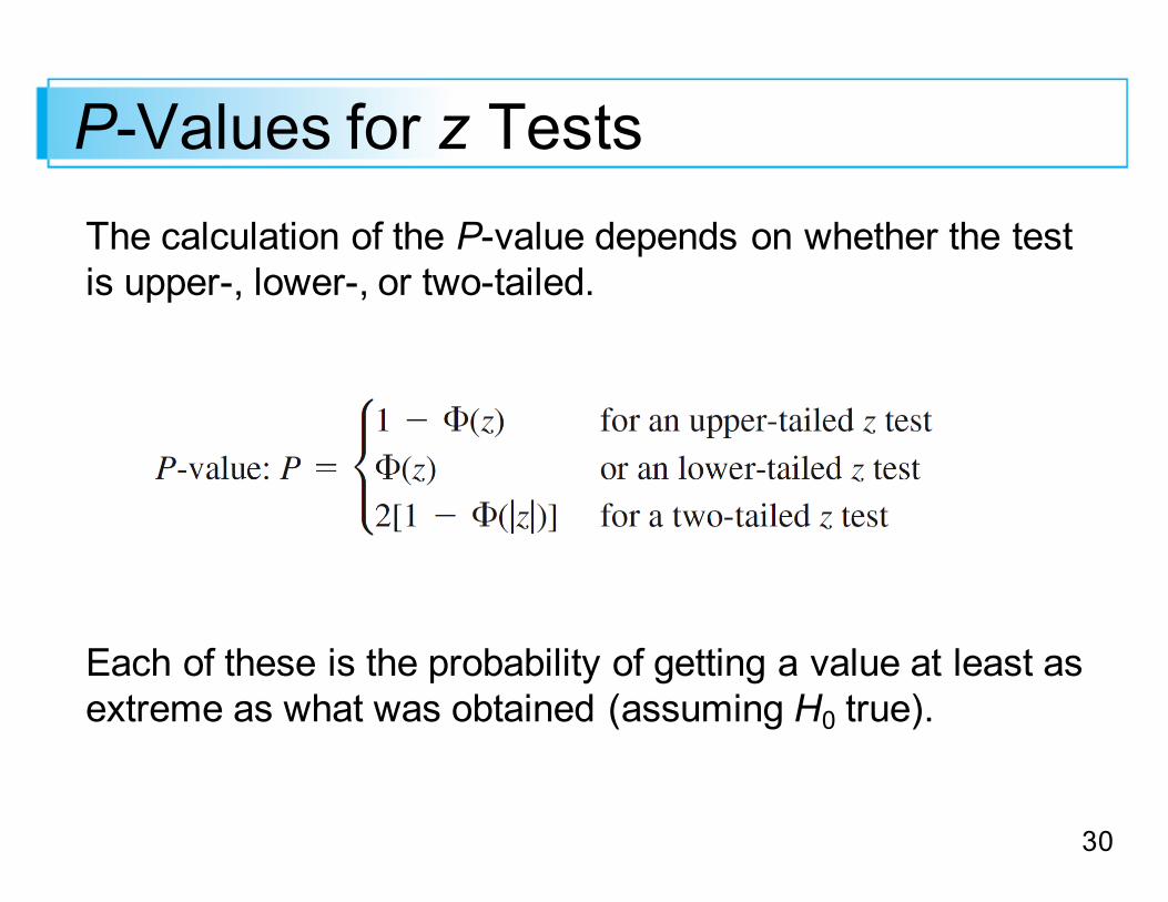
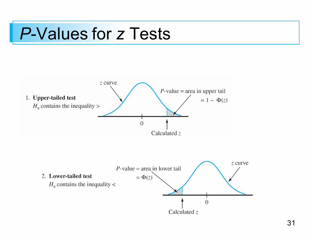
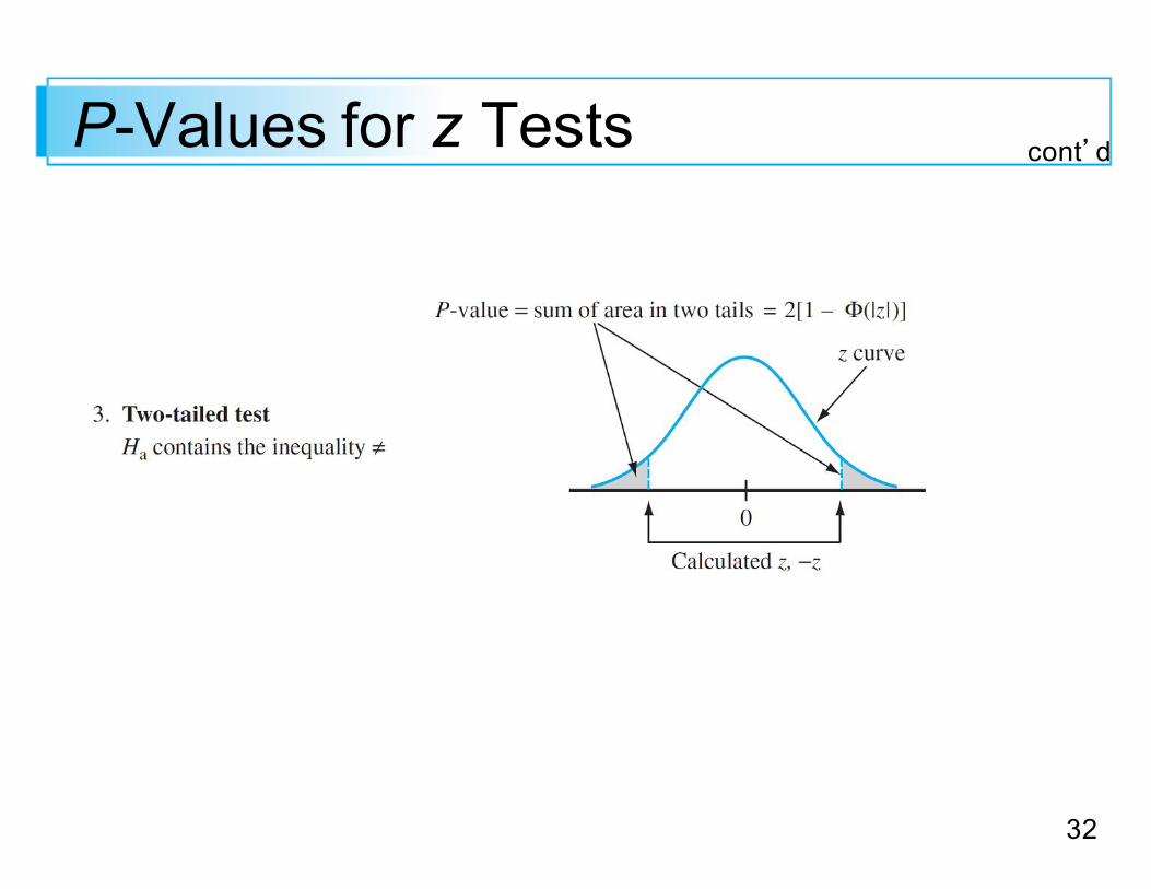
P-Values for z TestsThe calculation of the P-value depends on whether the test is upper-, lower-, or two-tailed.

Each of these is the probability of getting a value at least as extreme as what was obtained (assuming H0 true).

31

P-Values for z Tests

32

P-Values for z Tests cont’d

33

ExampleBack to the lawnmower engine example: There, we had

Ho: μ = 300 vs Ha: μ > 300and

Z = 1.18

What is the p-value for this result?

34

ExampleBack to the lawnmower engine example: There, we had

Ho: μ = 300 vs Ha: μ > 300and

Z = 1.18

Assuming our average doesn’t change much, what sample size would we need to see a statistically significant result?

35

ExampleBack to the Brinell scale example: There, we had

Ho: μ = 170 vs Ha: μ ≠ 170and

T = 2.19

What is the p-value for this result?

36

ExampleBack to the Brinell scale example: There, we had

Ho: μ = 170 vs Ha: μ ≠ 170and

T = 2.19

What if we had used alpha = 0.05 instead?

37

Distribution of p-valuesFigure below shows a histogram of the 10,000 P-values from a simulation experiment under a null μ = 20 (with n = 4 and σ = 2).

When H0 is true, the probability distribution of the P-value is a uniform distribution on the interval from 0 to 1.

38

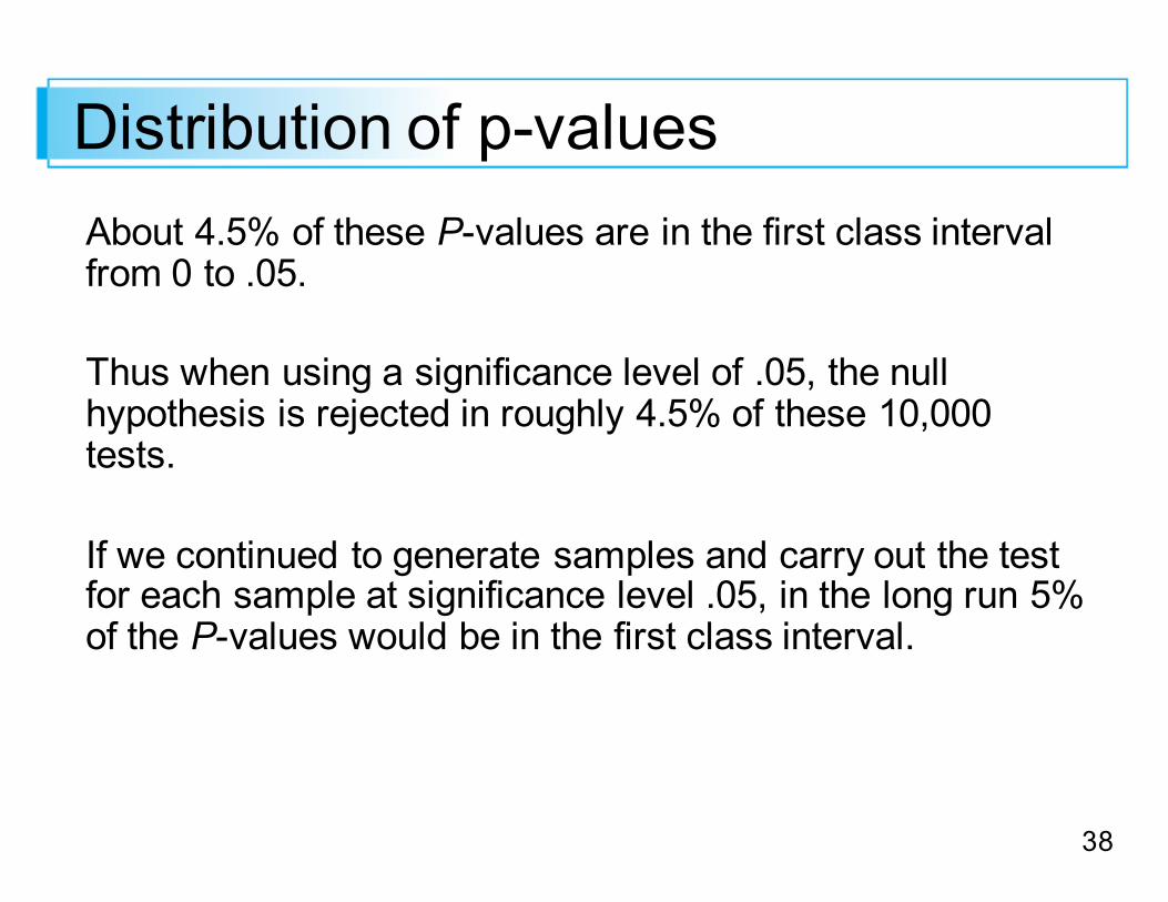
Distribution of p-valuesAbout 4.5% of these P-values are in the first class interval from 0 to .05.

Thus when using a significance level of .05, the null hypothesis is rejected in roughly 4.5% of these 10,000 tests.

If we continued to generate samples and carry out the test for each sample at significance level .05, in the long run 5% of the P-values would be in the first class interval.

39

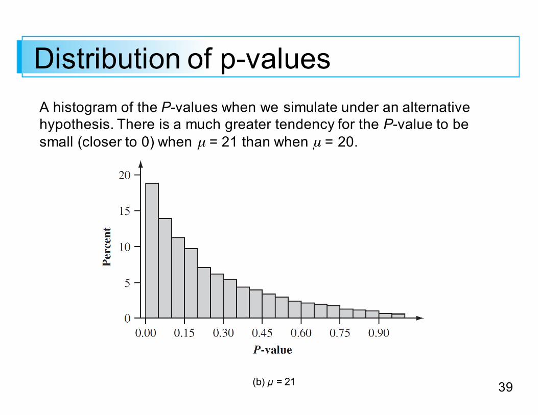
Distribution of p-valuesA histogram of the P-values when we simulate under an alternative hypothesis. There is a much greater tendency for the P-value to be small (closer to 0) when µ = 21 than when µ = 20.

(b) μ = 21

40

Distribution of p-valuesAgain H0 is rejected at significance level .05 wheneverthe P-value is at most .05 (in the first bin).

Unfortunately, this is the case for only about 19% of the P-values. So only about 19% of the 10,000 tests correctlyreject the null hypothesis;; for the other 81%, a type II error is committed.

The difficulty is that the sample size is quite small and 21 is not very different from the value asserted by the null hypothesis.

41

Distribution of p-valuesFigure below illustrates what happens to the P-value when H0 is false because µ = 22.

(c) μ = 22

42

Distribution of p-valuesThe histogram is even more concentrated toward valuesclose to 0 than was the case when µ = 21.

In general, as µ moves further to the right of the null value 20, the distribution of the P-value will become more and more concentrated on values close to 0.

Even here a bit fewer than 50% of the P-values are smaller than .05. So it is still slightly more likely than not that the null hypothesis is incorrectly not rejected. Only for values of µ much larger than 20 (e.g., at least 24 or 25) is it highly likely that the P-value will be smaller than .05 and thus give the correct conclusion.

43

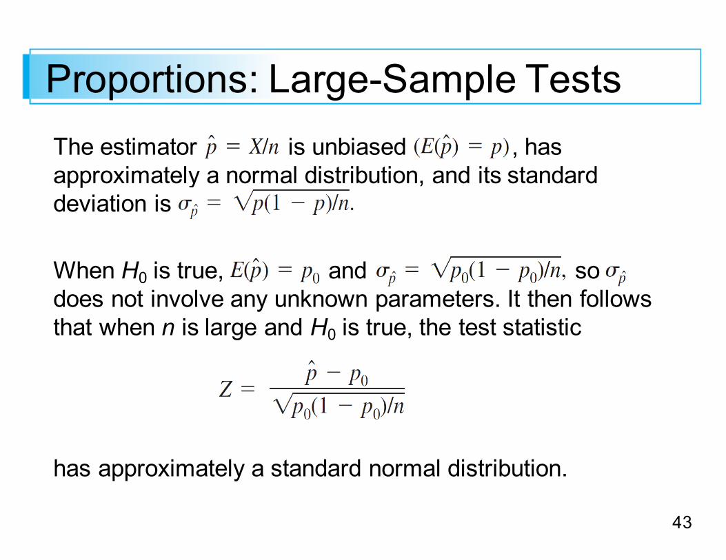
Proportions: Large-Sample TestsThe estimator is unbiased , has approximately a normal distribution, and its standard deviation is

When H0 is true, and so does not involve any unknown parameters. It then follows that when n is large and H0 is true, the test statistic

has approximately a standard normal distribution.

44

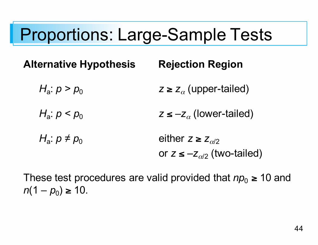
Proportions: Large-Sample TestsAlternative Hypothesis Rejection Region

Ha: p > p0 z ≥ zα (upper-tailed)

Ha: p < p0 z ≤ –zα (lower-tailed)

Ha: p ≠ p0 either z ≥ zα/2 or z ≤ –zα/2 (two-tailed)

These test procedures are valid provided that np0 ≥ 10 andn(1 – p0) ≥ 10.

45

Example Natural cork in wine bottles is subject to deterioration, and as a result wine in such bottles may experience contamination.

The article “Effects of Bottle Closure Type on Consumer Perceptions of Wine Quality” (Amer. J. of Enology and Viticulture, 2007: 182–191) reported that, in a tasting of commercial chardonnays, 16 of 91 bottles were considered spoiled to some extent by cork-associated characteristics.

Does this data provide strong evidence for concluding that more than 15% of all such bottles are contaminated in this way? Use a significance level equal to 0.10.

46

TWO SAMPLE TESTING

47

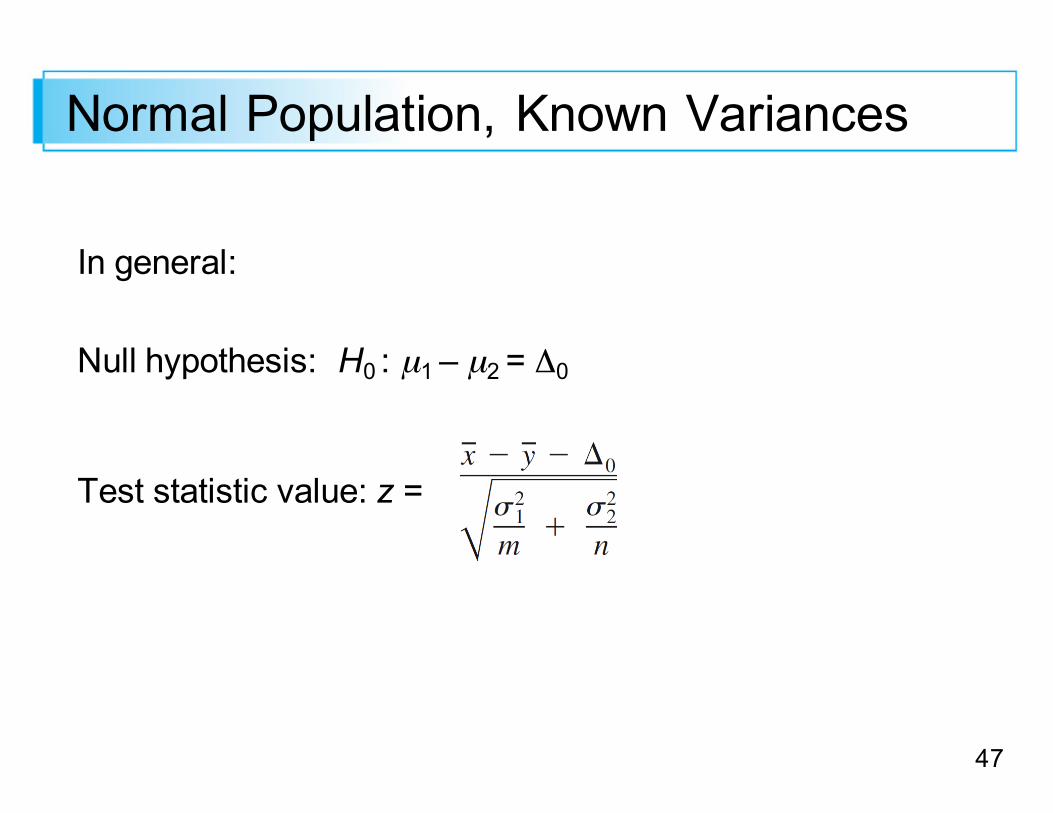
Normal Population, Known Variances

In general:

Null hypothesis: H0 : µ1 – µ2 = Δ0

Test statistic value: z =

48

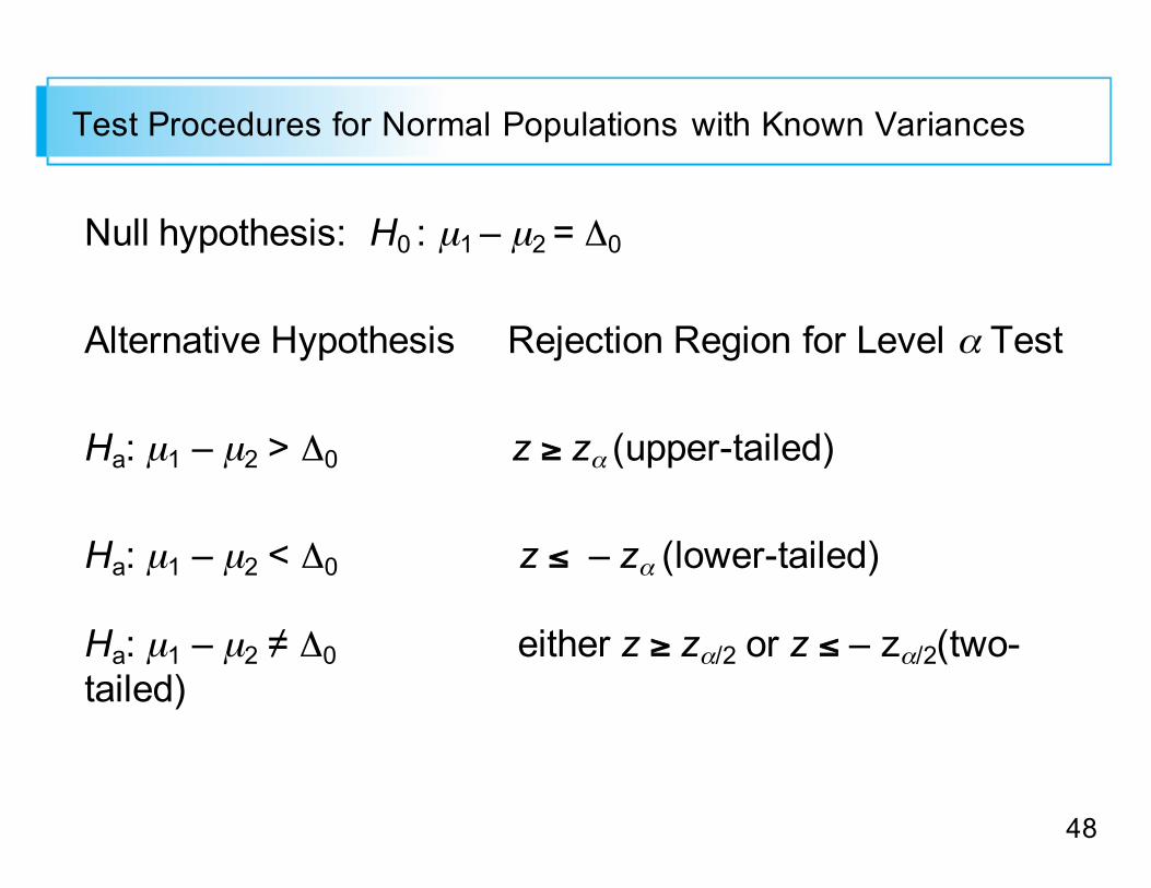
Test Procedures for Normal Populations with Known Variances

Null hypothesis: H0 : µ1 – µ2 = Δ0

Alternative Hypothesis Rejection Region for Level α Test

Ha: µ1 – µ2 > Δ0 z ≥ zα (upper-tailed)

Ha: µ1 – µ2 < Δ0 z ≤ – zα (lower-tailed)

Ha: µ1 – µ2 ≠ Δ0 either z ≥ zα/2 or z ≤ – zα/2(two-tailed)

49

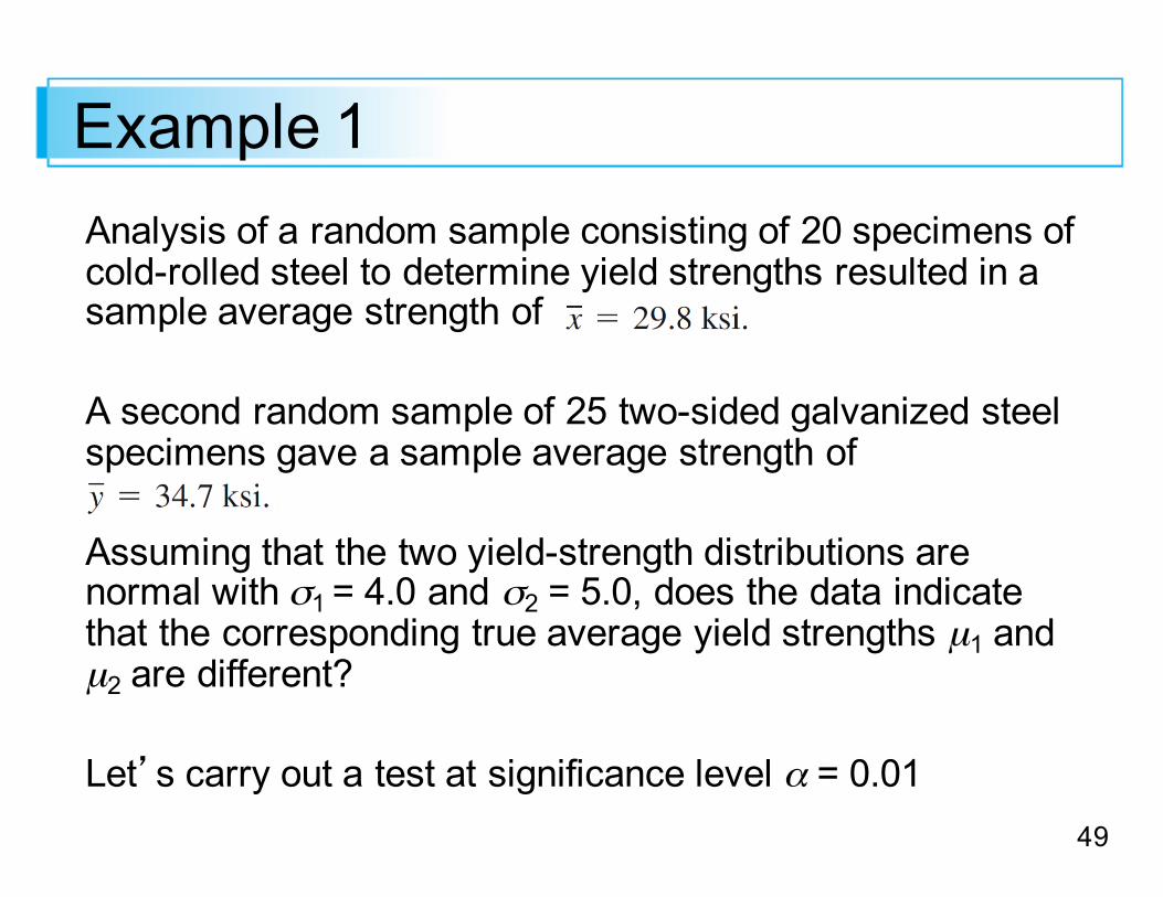
Example 1Analysis of a random sample consisting of 20 specimens of cold-rolled steel to determine yield strengths resulted in a sample average strength of

A second random sample of 25 two-sided galvanized steel specimens gave a sample average strength of

Assuming that the two yield-strength distributions are normal with σ1 = 4.0 and σ2 = 5.0, does the data indicate that the corresponding true average yield strengths µ1 and µ2 are different?

Let’s carry out a test at significance level α = 0.01

50

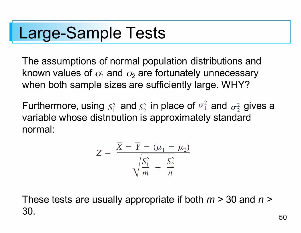
Large-Sample Tests The assumptions of normal population distributions and known values of σ1 and σ2 are fortunately unnecessary when both sample sizes are sufficiently large. WHY?

Furthermore, using and in place of and gives a variable whose distribution is approximately standard normal:

These tests are usually appropriate if both m > 30 and n >30.

51

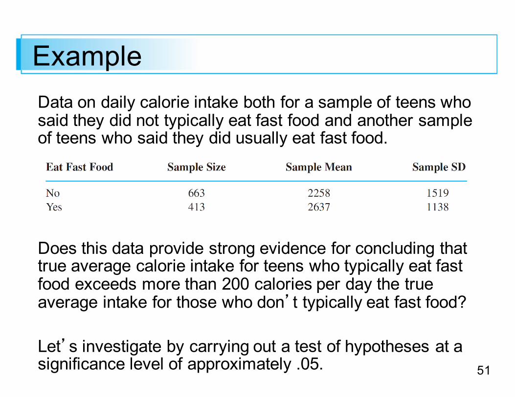
Example Data on daily calorie intake both for a sample of teens who said they did not typically eat fast food and another sample of teens who said they did usually eat fast food.

Does this data provide strong evidence for concluding that true average calorie intake for teens who typically eat fast food exceeds more than 200 calories per day the true average intake for those who don’t typically eat fast food?

Let’s investigate by carrying out a test of hypotheses at a significance level of approximately .05.

52

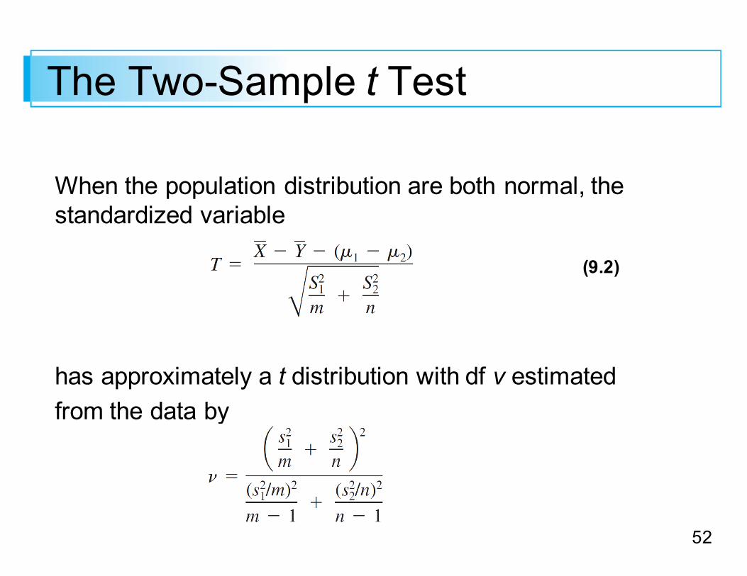
The Two-Sample t Test

When the population distribution are both normal, the standardized variable

has approximately a t distribution with df v estimated from the data by

(9.2)

53

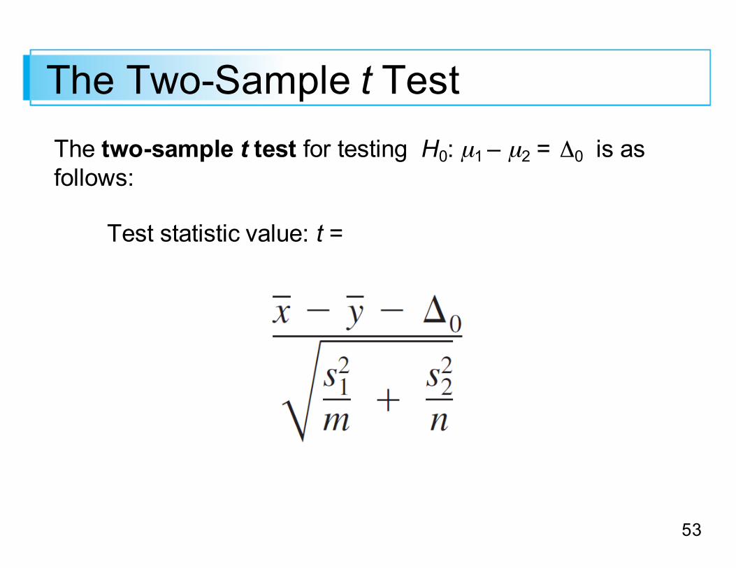
The Two-Sample t TestThe two-sample t test for testing H0: µ1 – µ2 = Δ0 is as follows:

Test statistic value: t =

54

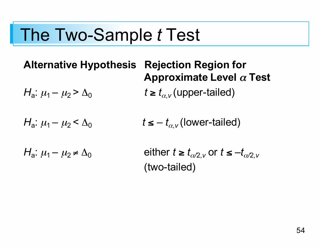
The Two-Sample t TestAlternative Hypothesis Rejection Region for

Approximate Level α TestHa: µ1 – µ2 > Δ0 t ≥ tα,v (upper-tailed)

Ha: µ1 – µ2 < Δ0 t ≤ – tα,v (lower-tailed)

Ha: µ1 – µ2 ≠ Δ0 either t ≥ tα/2,v or t ≤ –tα/2,v (two-tailed)

55

A Test for Proportion DifferencesTheoretically, we know that:

has approximately a standard normal distribution when H0is true.

However, this Z cannot serve as a test statistic because the value of p is unknown—H0 asserts only that there is a common value of p, but does not say what that value is.

56

A Large-Sample Test ProcedureUnder the null hypothesis, we assume that p1 = p2 = p, instead of separate samples of size m and n from two different populations (two different binomial distributions). So, we really have a single sample of size m + n from one population with proportion p.

The total number of individuals in this combined sample having the characteristic of interest is X + Y.

The estimator of p is then(9.5)

57

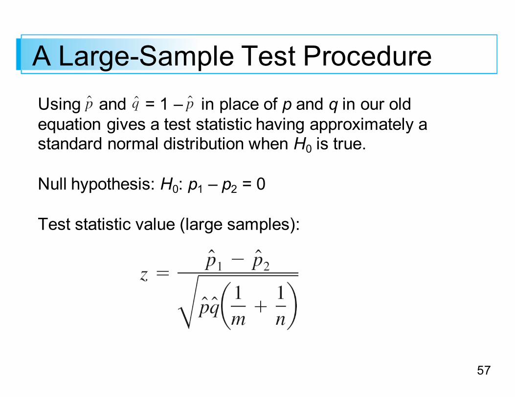
A Large-Sample Test ProcedureUsing and = 1 – in place of p and q in our old equation gives a test statistic having approximately a standard normal distribution when H0 is true.

Null hypothesis: H0: p1 – p2 = 0

Test statistic value (large samples):

58

A Large-Sample Test Procedure

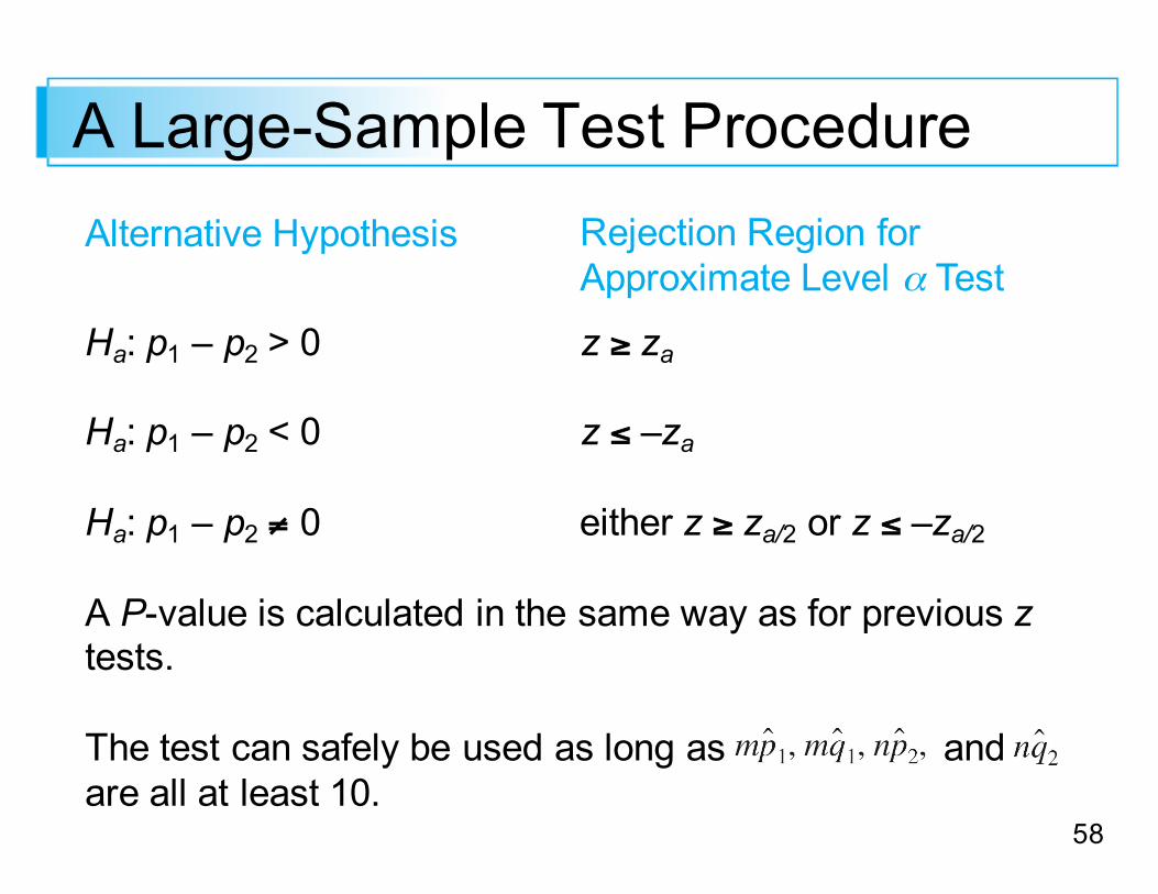
Ha: p1 – p2 > 0 z ≥ za

Ha: p1 – p2 < 0 z ≤ –za

Ha: p1 – p2 ≠ 0 either z ≥ za/2 or z ≤ –za/2

A P-value is calculated in the same way as for previous z tests.

The test can safely be used as long as andare all at least 10.

Alternative Hypothesis Rejection Region for Approximate Level α Test

59

The F Test for Equality of Variances

60

The F DistributionThe F probability distribution has two parameters, denoted by v1 and v2. The parameter v1 is called the numerator degrees of freedom, and v2 is the denominator degrees of freedom.

A random variable that has an F distribution cannot assume a negative value. The density function is complicated and will not be used explicitly, so it’s not shown.

There is an important connection between an F variable and chi-squared variables.

61

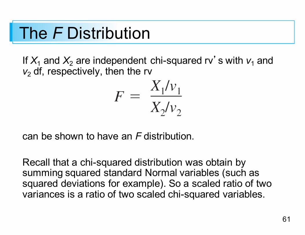
The F DistributionIf X1 and X2 are independent chi-squared rv’s with v1 and v2 df, respectively, then the rv

can be shown to have an F distribution.

Recall that a chi-squared distribution was obtain by summing squared standard Normal variables (such as squared deviations for example). So a scaled ratio of two variances is a ratio of two scaled chi-squared variables.

62

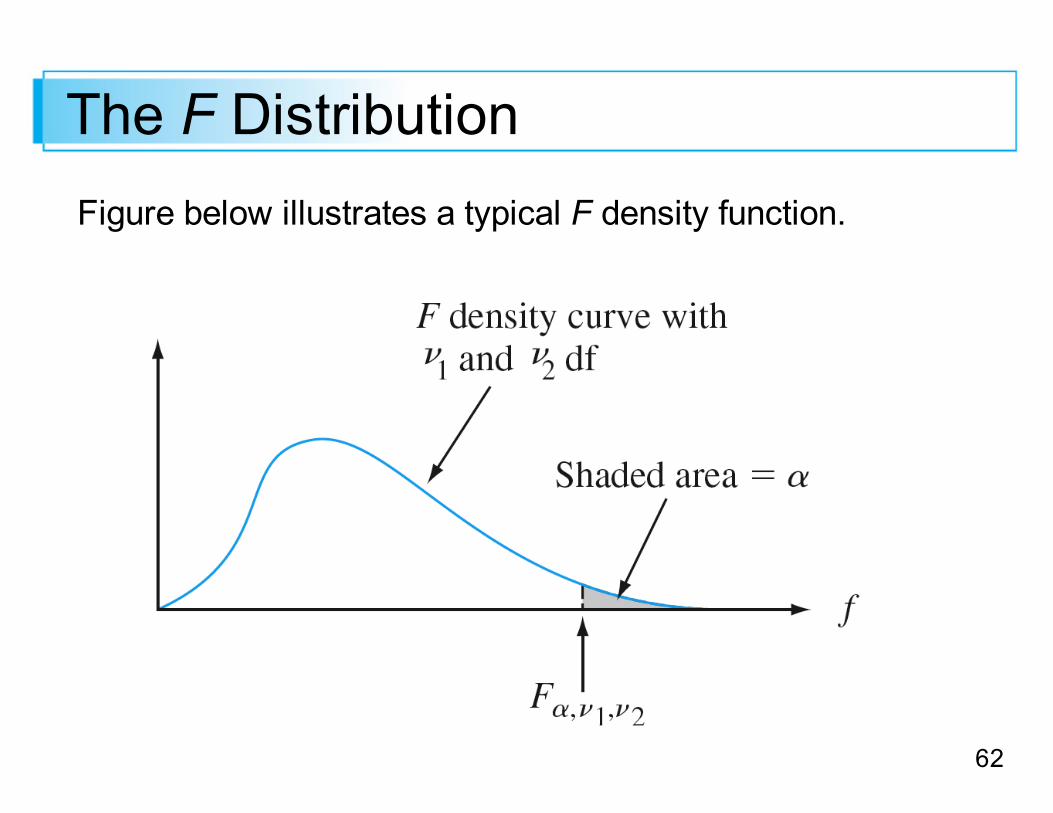
The F DistributionFigure below illustrates a typical F density function.

63

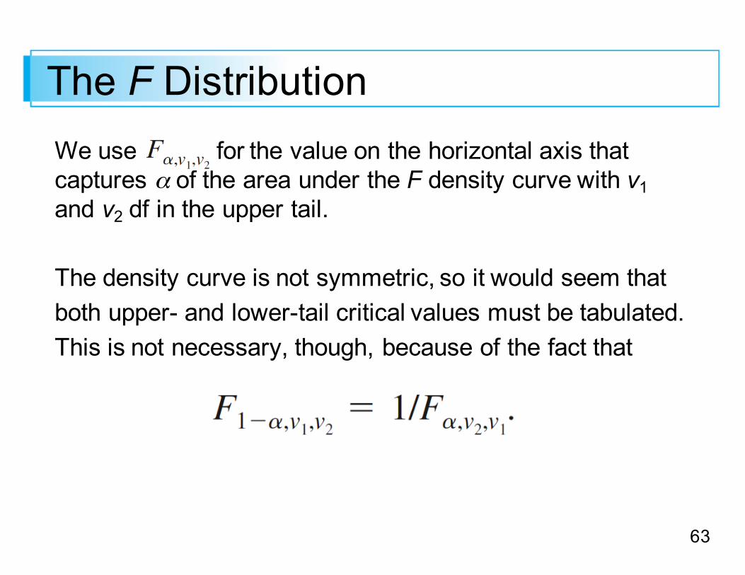
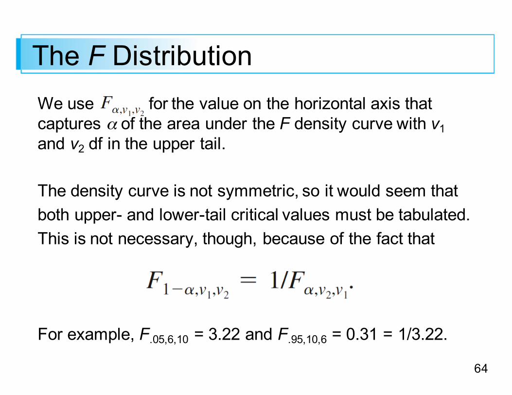
The F DistributionWe use for the value on the horizontal axis that captures α of the area under the F density curve with v1and v2 df in the upper tail.

The density curve is not symmetric, so it would seem that both upper- and lower-tail critical values must be tabulated. This is not necessary, though, because of the fact that

64

The F DistributionWe use for the value on the horizontal axis that captures α of the area under the F density curve with v1and v2 df in the upper tail.

The density curve is not symmetric, so it would seem that both upper- and lower-tail critical values must be tabulated. This is not necessary, though, because of the fact that

For example, F.05,6,10 = 3.22 and F.95,10,6 = 0.31 = 1/3.22.

65

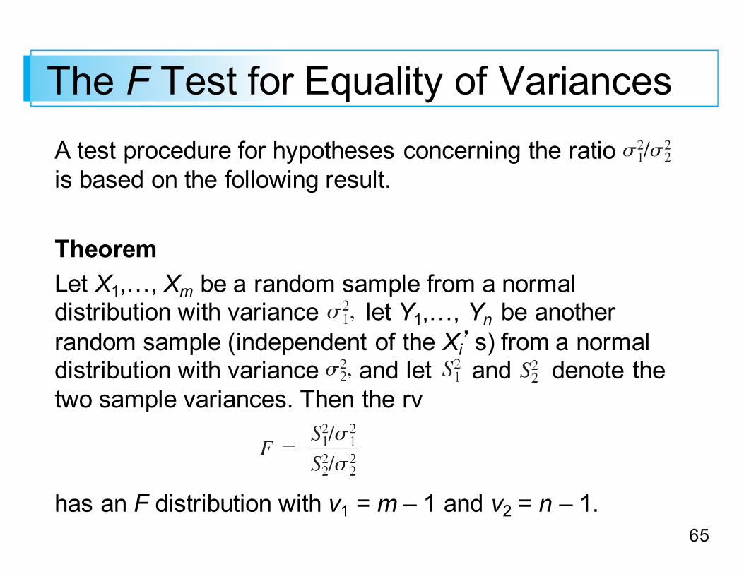
The F Test for Equality of VariancesA test procedure for hypotheses concerning the ratio is based on the following result.

TheoremLet X1,…, Xm be a random sample from a normal distribution with variance let Y1,…, Yn be another random sample (independent of the Xi’s) from a normal distribution with variance and let and denote the two sample variances. Then the rv

has an F distribution with v1 = m – 1 and v2 = n – 1.

66

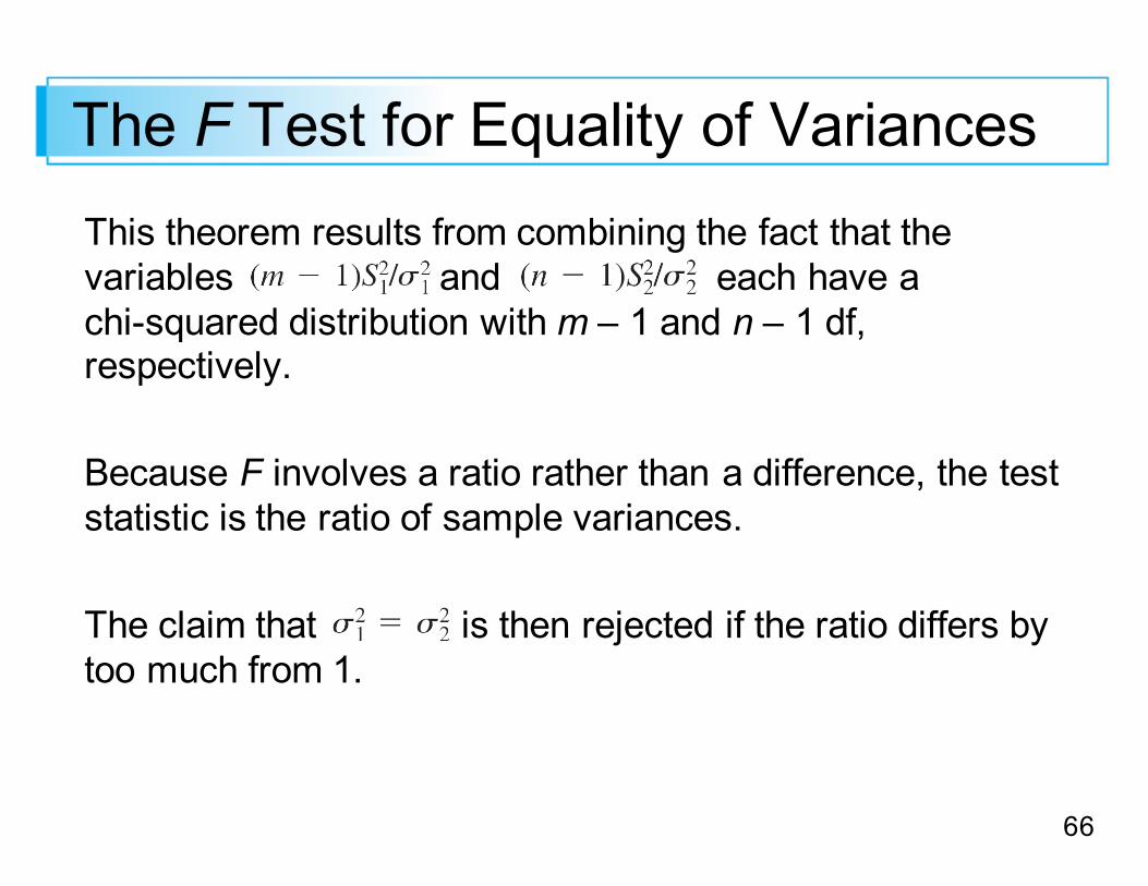
The F Test for Equality of VariancesThis theorem results from combining the fact that the variables and each have a chi-squared distribution with m – 1 and n – 1 df, respectively.

Because F involves a ratio rather than a difference, the test statistic is the ratio of sample variances.

The claim that is then rejected if the ratio differs by too much from 1.

67

The F Test for Equality of VariancesNull hypothesis:

Test statistic value:

Alternative Hypothesis Rejection Region for a Level αTest

68

Example On the basis of data reported in the article “Serum Ferritin in an Elderly Population” (J. of Gerontology, 1979: 521–524), the authors concluded that the ferritin distribution in the elderly had a smaller variance than in the younger adults. (Serum ferritin is used in diagnosing iron deficiency.)

For a sample of 28 elderly men, the sample standard deviation of serum ferritin (mg/L) was s1 = 52.6;; for 26 young men, the sample standard deviation was s2 = 84.2.

Does this data support the conclusion as applied to men? Use alpha = .01.

9 hypothesis*tests · 3 components*of*a*hypothesis*test 1. formulatethe*hypothesistobetested. 2....

Documents

9 hypothesistests · 3 componentsofahypothesistest 1. formulatethehypothesistobetested. 2....