851-0585-04l – modeling and simulating social …... modeling and simulating social systems with...
TRANSCRIPT

2012-11-12 © ETH Zürich |
851-0585-04L – Modeling and Simulating Social Systems with MATLAB
Lecture 8 – Continuous Simulations
© ETH Zürich |
Chair of Sociology, in particular of
Modeling and Simulation
Karsten Donnay and Stefano Balietti
2012-11-12 K. Donnay & S. Balietti / [email protected] [email protected] 2
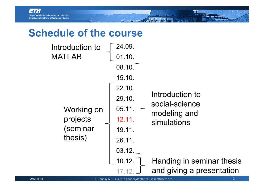
Schedule of the course 24.09. 01.10. 08.10. 15.10. 22.10. 29.10. 05.11. 12.11. 19.11. 26.11. 03.12. 10.12. 17.12.
Introduction to MATLAB
Introduction to social-science modeling and simulations
Working on projects (seminar thesis)
Handing in seminar thesis and giving a presentation

2012-11-12 K. Donnay & S. Balietti / [email protected] [email protected] 3
Schedule of the course 24.09. 01.10. 08.10. 15.10. 22.10. 29.10. 05.11. 12.11. 19.11. 26.11. 03.12. 10.12. 17.12.
Introduction to MATLAB
Working on projects (seminar thesis)
Handing in seminar thesis and giving a presentation
Dynamical Systems (no-space) Cellular Automata (grid)
Networks (graphs)
Continuous Space (…)
Different ways of Representing space

2012-11-12 K. Donnay & S. Balietti / [email protected] [email protected]
Goals of Lecture 8: students will 1. Consolidate knowledge acquired during lecture 7, through
brief repetition of the main points. 2. Receive an essential, but commensurate introduction
about Stochastic Processes. 3. Discover the Micro-Macro link in continuous modeling,
bridging Random Walk and Diffusion Equation. 4. Understand the basics of Motion Dynamics and learn
how to simulate processes like Brownian Motion in continuous space.
5. Have a closer glance into two examples of Pedestrian Simulation, confronting grids with continuous space.
4

2012-11-12 K. Donnay & S. Balietti / [email protected] [email protected]
Repetition - Generators Generating random, realistic graphs?
1. Probabilistic generators Erdos-Renyi: start with n nodes, connect with probability p
2. Degree-based generators Assign degrees to nodes; add edges, so that they match the original degree distribution
3. Process-based generators preferential attachment (Barabasi), attach new node:
5

2012-11-12 K. Donnay & S. Balietti / [email protected] [email protected]
Repetition We also saw a demonstration with Gephi
and some efficient network generating MATLAB functions
USE THEM and existing implementation from previous terms in your work (and cite them properly!)
6

2012-11-12 K. Donnay & S. Balietti / [email protected] [email protected]
All began with the Drunkard’s Walk The drunkard takes a series of steps away from
the lamp post, each with a random angle.
7
(Figure Resource: Sethna JP, 2006)

2012-11-12 K. Donnay & S. Balietti / [email protected] [email protected]
Stochastic Process A stochastic process:
(Xt)t ∈ I is a family of random variables indexed on an interval I , where I ⊂ R.
8
Intuitively, a stochastic process is an infinite- dimensional random vector
0 0.3 0.4 0.7 0.6 … 1 2 3 4 5

2012-11-12 K. Donnay & S. Balietti / [email protected] [email protected]
Stochastic Process In reality, we observe just a single realization of such
process, among all the possible ones. E.g. Stock Market Boom vs Stock Market Slump
9

2012-11-12 K. Donnay & S. Balietti / [email protected] [email protected]
White Noise (WN) White Noise is a stochastic process whose t-th
element has the following properties: E(xt) = 0 E(xt
2) = σ2 γk= 0 for |k| > 0 (autocorrelation coeff)
That means that the white noise is succession of uncorrelated random variables with zero mean and constant variance.
10

2012-11-12 K. Donnay & S. Balietti / [email protected] [email protected]
Random Walk (RW) Random Walk is a stochastic process whose t-
th element is determined as follows:
Xt = µ + Xt −1 + ϵt
µ is the drift, constantly leading the process towards its sign
ϵt represents the random increments.
11

2012-11-12 K. Donnay & S. Balietti / [email protected] [email protected]
Random Walk (RW)
12
function rw = rw(steps,drift) rw = zeros(steps,1); for i=2:steps rw(i) = drift + rw(i-1) + randn(1,1); end end
2012-11-12 K. Donnay & S. Balietti / [email protected] [email protected]
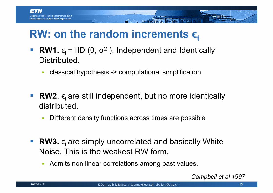
RW: on the random increments ϵt RW1. ϵt = IID (0, σ2 ). Independent and Identically
Distributed. classical hypothesis -> computational simplification
RW2. ϵt are still independent, but no more identically distributed. Different density functions across times are possible
RW3. ϵt are simply uncorrelated and basically White Noise. This is the weakest RW form. Admits non linear correlations among past values.
13
Campbell et al 1997

2012-11-12 K. Donnay & S. Balietti / [email protected] [email protected]
Random Walk and Diffusion Equation
14
Consider a general, uncorrelated random walk where at
each time step the particle’s position changes by
a step :
The probability distribution for each step is , which
has zero mean and standard deviation .

2012-11-12 K. Donnay & S. Balietti / [email protected] [email protected]
From Random Walk to Diffusion Equation For the particle to go from at time to at time ,
the step . Such event occurs with probability
times the probability density . Therefore,
we have
15

2012-11-12 K. Donnay & S. Balietti / [email protected] [email protected]
The Micro-Macro Link Using Taylor expansion, we have
16
The following is the diffusion equation

2012-11-12 K. Donnay & S. Balietti / [email protected] [email protected]
The Micro-Macro Link: Take Home Msg Diffusion:
Constant drift of the ensemble with the characteristic
constant D given by the properties of RW
A simple and controllable process such as RW applied to
single agents can give rise to seemingly organized
macroscopic behavior of the ensemble.
17
€
∂ρ∂t
=α 2
2Δt∂2ρ∂x 2
Diffusion Constant D
Differential Term for Diffusion

2012-11-12 K. Donnay & S. Balietti / [email protected] [email protected]
The Taylor Series The Taylor series is an approximation of a
function as an infinite sum of terms calculated from the values of its derivatives at a single point.
F(x) can thus be rewritten as:
18
a = single point
2012-11-12 K. Donnay & S. Balietti / [email protected] [email protected]
The Taylor Series in Matlab
19
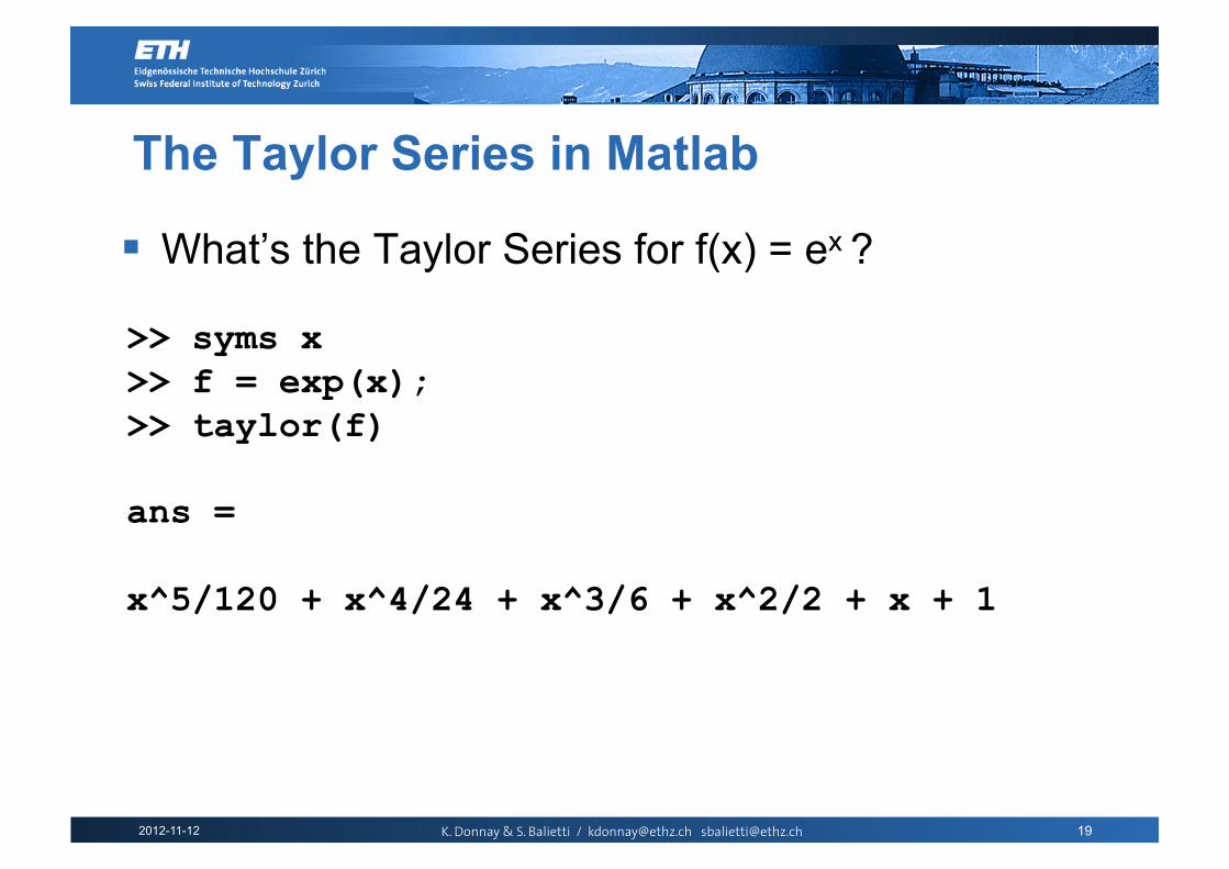
>> syms x >> f = exp(x); >> taylor(f)
ans =
x^5/120 + x^4/24 + x^3/6 + x^2/2 + x + 1
What’s the Taylor Series for f(x) = ex ?

2012-11-12 K. Donnay & S. Balietti / [email protected] [email protected]
The Taylor Series in Matlab
20
>> syms x >> f = exp(x); >> taylor(f)
ans =
x^5/120 + x^4/24 + x^3/6 + x^2/2 + x + 1
What’s the Taylor Series for f(x) = ex ?
And this is good because we reduced the complexity of the function from exponential to polinomial!

2012-11-12 K. Donnay & S. Balietti / [email protected] [email protected]
The Taylor Series in Matlab
21
Play with taylortool to get familiar Taylor Series

2012-11-12 K. Donnay & S. Balietti / [email protected] [email protected]
The Continuity Assumption
22
Resources: Google

2012-11-12 K. Donnay & S. Balietti / [email protected] [email protected]
From discrete to continuous space
Cellular automaton (CA)
Continuous simulation

2012-11-12 K. Donnay & S. Balietti / [email protected] [email protected]
Modelling motion in continuous space
Agents are characterized by:
position - X (m) - Y (m)
velocity - Vx (m/s) - Vy (m/s)
x
y
Vx
Vy

2012-11-12 K. Donnay & S. Balietti / [email protected] [email protected]
Modelling motion in continuous space
Next position after 1
second is given by:
x(t+1) = x(t) + Vx(t)
y(t+1) = y(t) + Vy(t)
x
y
Vx
Vy
Time t Time t+1

2012-11-12 K. Donnay & S. Balietti / [email protected] [email protected]
Modelling motion in continuous space
Time step dt is often
different from 1:
x(t+dt) = x(t) + dt Vx(t)
y(t+dt) = y(t) + dt Vy(t)
x
y
Vx
Vy
Time t Time t+dt dt<1
Time t+dt dt>1
2012-11-12 K. Donnay & S. Balietti / [email protected] [email protected]
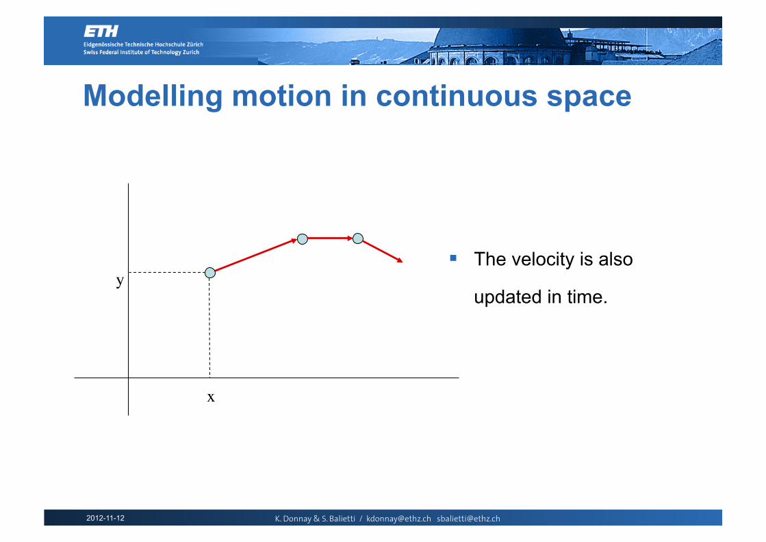
Modelling motion in continuous space
The velocity is also
updated in time.
x
y

2012-11-12 K. Donnay & S. Balietti / [email protected] [email protected]
Modelling motion in continuous space
The velocity changes as a result
of inter-individual interactions
Repulsion
Attraction
Examples: atoms, planets,
pedestrians, animals swarms…

2012-11-12 K. Donnay & S. Balietti / [email protected] [email protected]
Modelling motion in continuous space
The changes of the velocity
vector is defined by an
acceleration.

2012-11-12 K. Donnay & S. Balietti / [email protected] [email protected]
Modelling motion in continuous space
The velocity changes as a
result of interactions with the
environment
Repulsion
Attraction
Examples: bacteria, ants, pedestrian trails …

2012-11-12 K. Donnay & S. Balietti / [email protected] [email protected]
Modelling motion in continuous space
The velocity changes as a
result of a random process:
With or without bias
Example: exploration behaviour in many species of animals
2012-11-12 K. Donnay & S. Balietti / [email protected] [email protected]
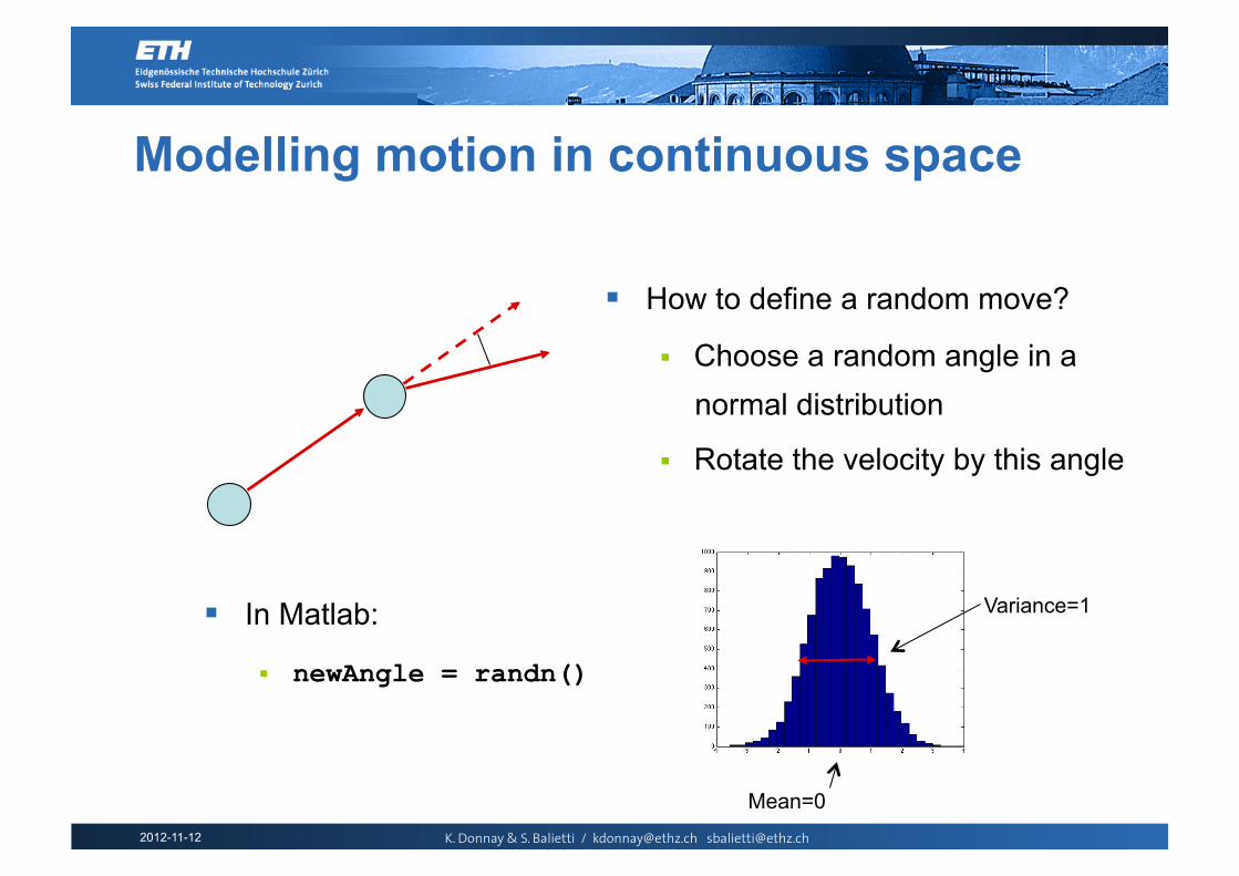
Modelling motion in continuous space
How to define a random move?
Choose a random angle in a normal distribution
Rotate the velocity by this angle
In Matlab:
newAngle = randn()
Mean=0
Variance=1

2012-11-12 K. Donnay & S. Balietti / [email protected] [email protected]
Modelling motion in continuous space
In Matlab:
meanVal=2;
v=0.1;
newAngle = meanVal + v*randn()
How to define a random move?
Choose a random angle in a normal distribution
Rotate the velocity by this angle
2012-11-12 K. Donnay & S. Balietti / [email protected] [email protected]
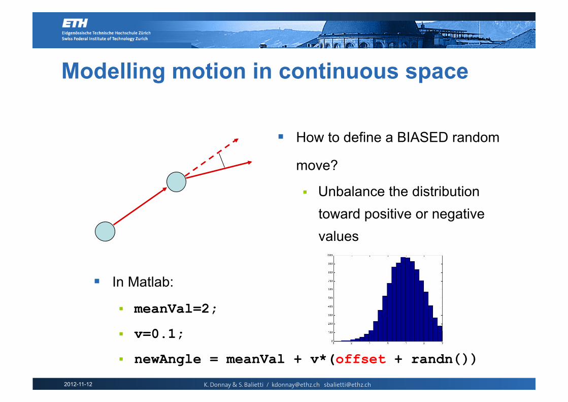
Modelling motion in continuous space
How to define a BIASED random
move?
Unbalance the distribution toward positive or negative values
In Matlab:
meanVal=2;
v=0.1;
newAngle = meanVal + v*(offset + randn())

2012-11-12 K. Donnay & S. Balietti / [email protected] [email protected]
Programming a Continuous Simulator
X = [1 1 3 ]; Y = [2 1 1]; Vx = [0 0 0.1]; Vy = [1 1 0.5];
for t=1:dt:T for p=1:N [Vx(p) Vy(p)] = update( …) ; X(p) = X(p) + dt*Vx(p) ; Y(p) = Y(p) + dt*Vy(p) ; end
end
Initialization: Four elements are required to define the state of individuals
The velocity is updated first, and then the position as a function of the velocity and the time step

2012-11-12 K. Donnay & S. Balietti / [email protected] [email protected] 36 36
Brownian Motion %Brownian Motion!t = 100;n = 1000;dt=t/n;!x = zeros(1,n);!y = zeros(1,n);!dx = zeros(1,n);!dy = zeros(1,n);!x(1) = 0;y(1) = 0;!hold on;!k = 1;!for j=2:n! x(j)= x(j-1) +…! sqrt(dt)*randn;! y(j)= y(j-1) +…! sqrt(dt)*randn;! plot([x(j-1),x(j)],…! [y(j-1),y(j)]);!! k = k + 1;!end!

2012-11-12 K. Donnay & S. Balietti / [email protected] [email protected] 37
Pedestrian Simulation
CA model
Many-particle model

2012-11-12 K. Donnay & S. Balietti / [email protected] [email protected] 38
CA Model (A. Kirchner, A. Schadschneider, Phys. A, 2002)
2012-11-12 K. Donnay & S. Balietti / [email protected] [email protected] 39
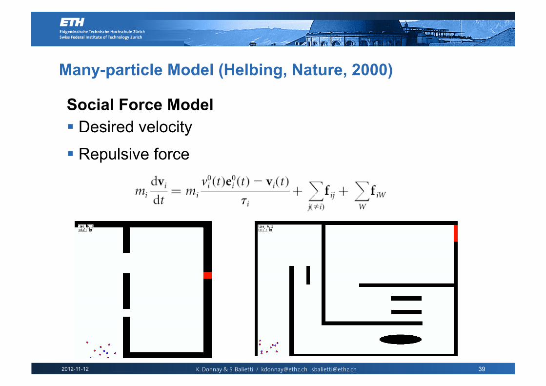
Many-particle Model (Helbing, Nature, 2000)
Social Force Model Desired velocity
Repulsive force

2012-11-12 K. Donnay & S. Balietti / [email protected] [email protected]
Easier
Implementation dependant
More Limited
One Element per Cell
Computationally more
intensive
(more) Complex
Elegant
Extremely Powerful
Agents Float in Space
Computationally faster
(with analytical derivates)
40
Grids Vs Continuum Space

2012-11-12 K. Donnay & S. Balietti / [email protected] [email protected]
Easier
Implementation dependant
More Limited
One Element per Cell
Computationally more
intensive
(more) Complex
Elegant
Extremely Powerful
Agents Float in Space
Computationally faster
(with analytical derivates)
41
Grids Vs Continuum Space
You can write a good paper with both approaches if you have a good idea

2012-11-12 K. Donnay & S. Balietti / [email protected] [email protected]
Train Boarding Simulation (Graf & Krebs, Fall 2010)
42
Examples from Previous Semesters
2012-11-12 K. Donnay & S. Balietti / [email protected] [email protected]
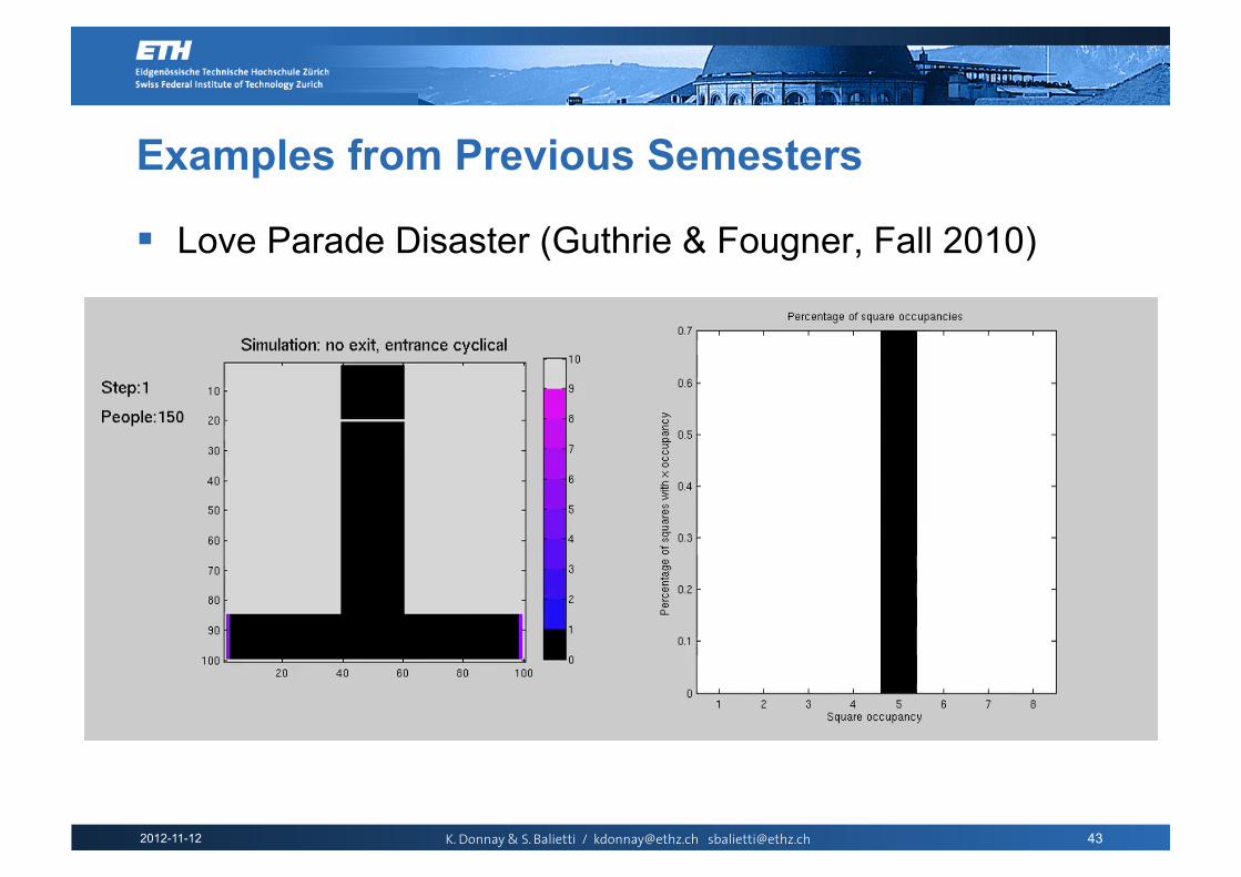
Love Parade Disaster (Guthrie & Fougner, Fall 2010)
43
Examples from Previous Semesters

2012-11-12 K. Donnay & S. Balietti / [email protected] [email protected]
Airplane Evacuation (Bühler & Heer, Spring 2011)
44
Examples from Previous Semesters

2012-11-12 K. Donnay & S. Balietti / [email protected] [email protected]
Flooding Evacuation (Crameri & Thielmann, Fall 2011)
45
Examples from Previous Semesters

2012-11-12 K. Donnay & S. Balietti / [email protected] [email protected]
Desert Ant Navigation (Megaro & Rudel, Fall 2011)
46
Examples from Previous Semesters

2012-11-12 K. Donnay & S. Balietti / [email protected] [email protected]
Projects Today, there are no exercises. You can work on your projects and we will
supervise you.
If you have preliminary results we are happy to discuss them with you…
47

2012-11-12 K. Donnay & S. Balietti / [email protected] [email protected]
References http://en.wikipedia.org/wiki/Taylor_expansion
http://en.wikipedia.org/wiki/Random_walk
Toolbox for different random walks:
http://www.mathworks.com/matlabcentral/fileexchange/22003
Nature 407, 487-490 (2000) Simulating dynamical features of
escape panic. Dirk Helbing, Illés Farkas and Tamás Vicsek
The Econometrics of Financial Markets. 1997. John Y. Campbell,
Andrew W. Lo, A. Craig MacKinsley. Princeton University Press.
48

2012-11-12 K. Donnay & S. Balietti / [email protected] [email protected]
GitHub Links Train Boarding Simulation (Graf & Krebs, Fall 2010)
https://github.com/msssm/Train-Boarding
Love Parade Disaster (Guthrie & Fougner, Fall 2010) https://github.com/msssm/Love_Parade_2010
Airplane Evacuation (Bühler & Heer, Spring 2011) https://github.com/msssm/Airplane_Evacuation_2011_FS
Flooding Evacuation (Crameri & Thielmann, Fall 2011) https://github.com/mthielma/SOCIAL_MODELING
Desert Ant Navigation (Megaro & Rudel, Fall 2011) https://github.com/erudel/desert_ant_behavior_gordonteam
49