SANDIA REPORT SAND83–1909 ● Unlimited Release ● UC–60

Printed September 1984

Modeling Stochastic Wind Loads, on Vertical Axis Wind Turbines

Prepared by

Sandia National LaboratoriesAlbuquerque, New Mexico 87185 and Livermore, California 94550for the United States Department of Energy

under Contract CIE-AC04-76DPO0789

Issued by .%rdiaNationalLaboratories,operatedforthe UnitedStatesDepartmentofEnergyby SandiaCorporation.NOTICE Thisreportwaspreparedasanaccountofworksponsoredby anagencyoftheUnitedStatesC,overnment.NeithertheUnitedStatesGovern-ment norany agencythereof,norany oftheiremployees,norany oftheircontractors,subcontractors,or theiremployees,makes any warranty,ex-pressor implied,or aaaumesany legalliabilityor responsibilityfortheaccuracy,completeness,orusefulnessofany information,apparatus,prod-uct,or processdisclosed,or representathatitause would not infringeprivatelyowned rightsReferencehereintoanyspecificcommercialproduct,process,orserviceby tradename,trademark,manufacturer,or otherwise,doesnotnecessarilyconstitukorimplyitaendorsement,recommendation,orfavoringby theUnitedStatesGovernment,any agencythereoforany oftheircontractorsorsubcontractors.The viewsand opinionsexpressedhere-indo notnecessarilystateorreflectthoseoftheUnitedStatesGovernment,any agencythereoforany oftheircontractorsorsubcontractors.

Printed intheUnitedStatesofAmericaAvailablefromNationalTechnicalInformationServiceU.S.DepartmentofCommerce5285PortRoyalRoadSpringfield,VA 22161

NTIS pricecedesPrintedcopy A19Microfichecopy AO1

MODELING STOCHASTIC WIND LOADS

ON VERTICAL AXIS WIND TURBINES

Paul S. Veers

Applied Mechanics Division 1524Sandia National Laboratories

Albuquerque, New Mexico

Abstract

The Vertical AXIS Wind Turbine (VAWT) is a machine which extracts energyfrom the wind. Since random turbulence is always present, the effect of

this turbulence on the wind turbine fatigue life must be evaluated. This

problem 1s approached by numerically simulating the turbulence and calcu–

latlng, In the time domain, the aerodynamic loads on the turbine blades.

These loads are reduced to the form of power and cross spectral densitieswhich can be used In standard linear structural analysls codes. The rela-

tive Importance of the turbulence on blade loads 1s determined.

The most common des]gn for Vertical Axis Wind

Turb]nes (VAWT’S) was first patented in 1931 byDarrleus, a Frenchman. Th]s “egg beater” shaped

machine consists of one or more blades with air–foil cross sections attached to the top and bottomof a central shaft, or tower. To m]nlmize bendingstresses In the blades while the turbine rotates,

the blades usually have a characteristic tropos–klen, or “splnnlng rope,” shape. Torque is

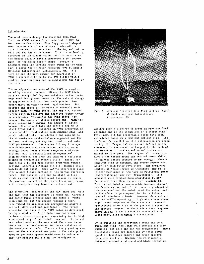
produced when the turb]ne rotor turns In the wind.Fig. 1 shows the 17 meter research VAWT at SandlaNational Laboratories, Albuquerque, NM Thisturb]ne has the most common configuration ofVAWT’S currently being built, two blades w]th a

central tower and guy cables supporting the top of

the rotor.

The aerodynamic analysls of the VAWT 1s compli–cated by several factors Since the VAWT blade

rotates through 360 degrees relatlve to the lncl–dent wind during each rotation, the rate of changeof angle of attack 1s often much greater thanexperienced ]n other airfoil applications. But

because the speed of the blade 1s normally much

greater than the w]nd speed, the angle of attackvaries between posltlve and negative values around

zero degrees. The higher the w]nd speed, thegreater the angle of attack excursions. When thewinds become h]gh enough, the angles of attackbecome large enough that the alrfoll begins tostall dynamically. Research In VAWT aerodynamics1s currently lnvestlgatlng both dynamic stall and

p]tch rate effects. Aerodynrunlc analys]s using

the streamtube momentum balance approach was theearnest and slm lest approach used to est]mate

YVAWT performance The vortex llftlng llne ap–

preach has produced some better results, in anaverage sense, over a wider range of wlnd2con-d]tlons, but 1s computatlonally expensive

Both methods suffer from the lack of a valldatedmethod of predicting dynemlc stall. Except foremplrlcal llft and drag curves from wind tunneltesting, accurate pltchlng airfoil, dynamic stall

models do not exist. Most VAWT’S experience stallover a s]gnlflcant portion of the normal operat]ngrange The loss of llft due to stall in highwinds 1s considered benef]clal because It llmlts

the maximum power that the drive train must trans–mlt, thereby holding down the turbine cost.

The structural analysls of the VAWT must deal with

the fact that the structure is rotating. Corlollsand centrifugal effects make the modes of vlbra–tlon complex, but the system remains l]near.

Free v]bratlon analysls and aero lastlc analysis5

are well developed and valldated The forcedv]bratlon analysis of the VAWT rotor ]s developed,

but agreement w]th field data from operating

turbines 1s sometimes poor, especlall~ In the high

w]nd speed, significant stall, regime It is notyet clear whether the source of the error 1s In

the structural analysls or ]n the calculation ofthe aerodynem]c loads The relatively good agree–

ment of the structural analysis to the data gath-ered at low wind speeds would seem to indicate

that the problem may l]e in the aerodynamics.

Fig. 1 Darrleus Vertical AXIS Wind Turb]ne (VAWT)at Sand]a National Laboratories,

Albuquerque, NM

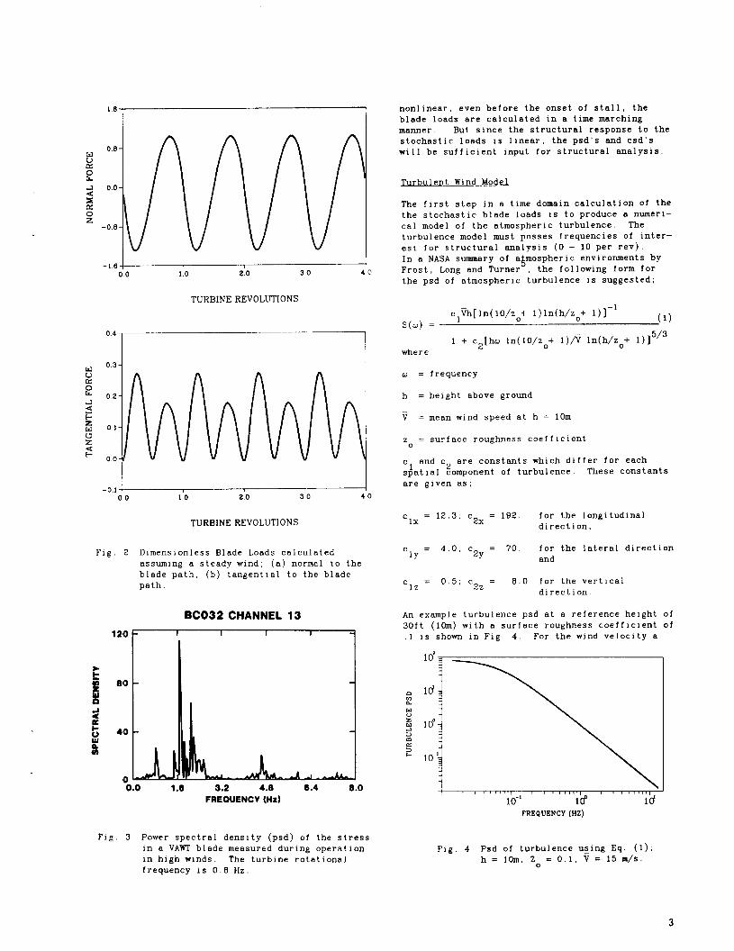
Another possible source of error In previous loadcalculations 1s the assumption of a steady w]nd.

Until now, all the aerodynamic loads have beencalculated based on a constant emblent wind. The

loads which result from this calculation are shown

In Fig. 2. Tangential forces are def]ned as thecomponent In the dlrect]on tangent to the path ofthe blade as It rotates and normal forces arenormal to this path. The tangential forces pro–

duce a net torque about the central tower whilethe normal forces produce no net energy. When aconstant wind lS assumed, the forces repeat ex-

actly for each rotor revolution. The frequency

content of these forces 1s therefore limlted to

Integer mult;ples of the turbine rotational speed(abbreviated as “per rev” frequencies). This

approach will produce zero excltat]on at anyfrequency other than the per rev frequencies.

This lS not totally unreasonable because the perrev frequency content of the loads 1s produced bythe mean wind and the rotation of the rotor, and]s therefore large compared to the turbulence

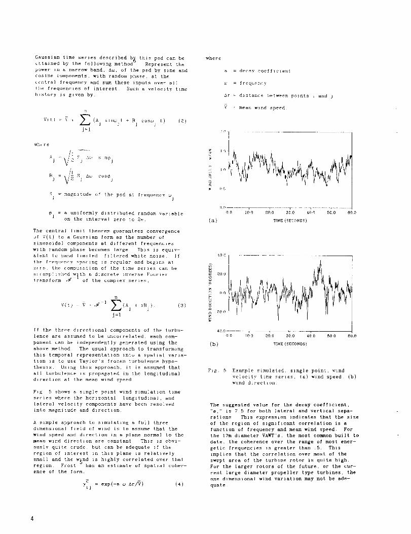
induced, stochastic loads However, data collect-ed from VAWT’S operat]ng in high winds have shownslgnlf]cant response at the structural resonant

frequencies as well as at the per rev frequencies.The spectral content of the blade stress responseshown in Flg 3 could never be predicted with

loads calculated assuming e steady wind.

By calculating the aerodynamic loads due to aturbulent wind, the loads will contain all fre–

quencles, not only the per rev frequencies. These

stochastic loads are described by their power

spectral densities (psd’s) and cross spectraldensltles (csd’s). Because the relationship

between incident wind speed and blade forces is

2

-1.64 \ I00 10 20 30 49

nonlinear, even before the onset of stall, theblade loads are calculated in a time marchingmanner But since the structural response to thestochastic loads is linear, the psd’s and csd’s

will be sufficient input for structural analysis.

J’urbulent Wind Model

TURBINE REVOLUTIONS

clfi[ln(]O/zo+ l)ln(h/zo+ 1)]–1

S(Q) =(1)

1 + c2[hti ln(lO/zo+ 1)/~ ln(h/zo+ 1)]5/3

where

TURBINE REVOLUTIONS

Fig. 2 Dlmenslonless Blade Loads calculatedassuming a steady wind, (a) normal to the

12(D

so

4{D

n

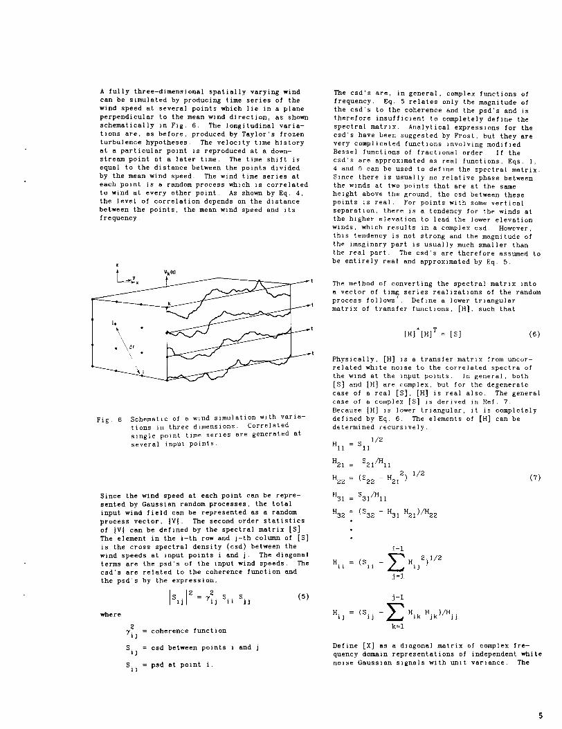
The first step in a time domain calculation of thethe stochastic blade loads IS to produce a numeri-cal model of the atmospheric turbulence. The

turbulence model must posses frequencies of inter-est for structural analysls (O – 10 per rev).In a NASA summary of a mospheric environments by

kFrost, Long and Turner , the followlng fOrm for

the psd of atmospheric turbulence is suggested;

.oll~0.0 Lo 20 30 40

blade path, (b) tangential to the bladepath.

BC032 CHANNEL 13

1- 1 I I I =i

-i)mo 1.6 3.2 4.8 6.4 8.0FREQUENCY

Fig. 3 Power spectral density (psd) of the stress

in a VAWT blade measured during operationIn high winds. The turbine rotationalfrequency 1s 0.8 Hz,

u = frequency

h = height above ground

~ = mean wind speed at h = 10m

z = surface roughness coefficient0

c1and c are constants which differ for each

spatial ~omponent of turbulence. These constants

are given as;

Clx= 12.3, C2X = 192. for the longitudinal

direction,

Cly= 4.0, c = 70.

2yfor the lateral directionand

Clz = 0“5’ C2Z =8.0 for the vert)cal

direction.

An example turbulence psd at a reference height of30ft (lOm) with a surface roughness coeff]clent of.1 1s shown :n Fig. 4. For the wind velocity a

aw0.

lo’s

ld :

Io”z

10-‘:

f 110-’

[10° Id

FREQUENCY (HZ)

Fig. 4 Psd of turbulence using Eq. (l);

h=lom, Zo=0.1,V=15m/s.

3

Geussian time ser)es described b~ this psd can be

ct.talned by the followlng method” Represent thepower In a narrow band, &@, of the psd by s,n~ and

cosine components, with random phase, .gt the

rcntral frequency and sum these Inputs over al 1

the frequencies of Interest. Such a veloclty timehlstor’y 1s g]ven by,

[1

V(l)=v, x (AJ S]Ilti,t+ B COSU ~ t)(2)

1j=l

Wht’re

r,——

s = magnitude of the psd at frequency L!J J

$, = a uniformly distributed random variable

on the Interval zero to 2n,

The central llmlt. theorem guarantees convergence

Of ~(t) to a Gaussian form as the number ofslnllsoidal corrponents at different frequencieswith random phase becomes large, This ]s equlv–aler,t to band l]m] ted, f]ltered wh]te no]se Ifthe’ frequency spacing is regular and beg]ns at

zero. the compuiatlon of the time series can betif<omp] l~l)edw th 8 d]screte Inverse Fouriertrensform .#

-1of the complex series,

...v(t) = v +.x

-1

x(Aj + }Bj)

j=l

(3)

If the three directional components of the turbu–

lence are assumed to be uncorrelated, each com–ponent can be Independently generated using theabove method The usual approach to transformingth]s temporal representation Into a spatial var]a–tlon IS to use Taylor’s frozen turbulence hypo–thesis Using this approach, It 1s assumed thatall turbulence IS propagated in the longltudlnaJdlrectlon at the mean wind speed

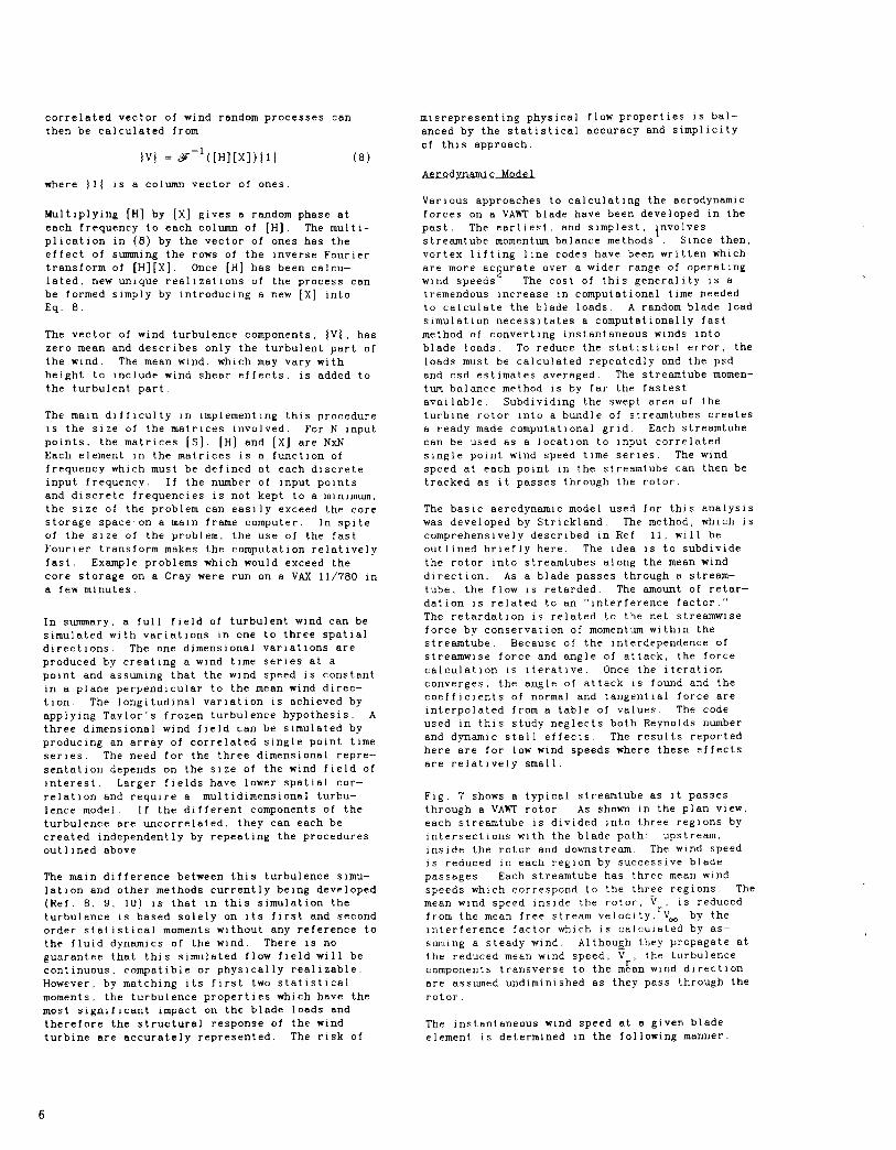
F]g 5 shows a single point wind simulation timeseries where the horizontal longltudlnal, andlateral veloclty components have been resolvedInto magnitude and dlrect]on.

A s]mple approach to simulating a full threedlmens]onal field of w]nd ]s to assume that thew)nd speed and dlrectlon In a plane normal to the

mean wind dlrectlon are constant. This IS obvl–OUSIV quite crude, but can be adequate If theregion of Interest In this plane 1s relativelysmall and the w nd IS h)ghly correlated over that

Frosti

region has an est]mate of spat]al coher–ence of the form,

7:J = exp(–a u Ar/~) (4)

where

a = decay coeff]c]ent

~ = frequvncv

l,r= distance between po]nts 1 and j

~= mean wind speed

Ili

1 ‘-”—~

(a)

no ;— ----—r—- —-+

00 100 200 300 400 60.0

TIME(sEcoNtIs)

40(17 - ——-—--”~I I

4 ~o~o,o-400 --–— -—T--—00 100

(b) TIME(SECONDS)

F]g. 5 Example simulated, single point, wind

veloc]ty time series, (a) w]nd speed, (b)wind dlrectlon

The suggested value for the decay coefficient,“a, “ 1s 7.5 for both lateral and vertical sepa–rations. This expression lndlcates that the size

of the reg]on of slgnlflcant correlation 1s afunction of frequency and mean wind speed. For

the 17m diameter VAW’i’s, the most common built to

date , the coherence over the range of most ener–

get]c frequencies IS greater than .5. This

Implles that the correlation over most of theswept area of the turbine rotor IS qu]te high.

For the larger rotors of the future, or the cur–rent large d]ameter propeller type turbines, theone d)mens]onal wind varlat]on may not be ade–

quate

A fully three–dimensional spatially varying windcan be simulated by producing time series of thewind speed at several points which lie in a plane

perpendicular to the mean wind direction, as shown

schematically in Fig. 6. The longitudinal varia–tions are, as before, produced by Taylor’s frozenturbulence hypotheses, The velocity time historyat a particular point 1s reproduced at a down–stream point at a later time. The time shift isequal to the distance between the points dividedby the mean wind speed. The wind time series ateach point )s a random process which is correlatedto wind at every other point. AS shown by Eq. 4,the level of correlation depends on the distancebetween the po:nts, the mean wind speed and itsfrequency.

z

L v~(t)Y Ax

Fig, 6 Schematic of a wind simulation with varla–tions in three dimensions. Correlated

single point time series are generated atseveral Input points.

Since the wind speed at each point can be repre–sented by Gaussian random processes, the total

input wind field can be represented as a randomprocess vector, {V]. The second order statistics

of {V} can be defined by the spectral matrix [s].The element In the i–th row and j-th column of [s]is the cross spectral density (csd) between the

wind speeds at input points i and j The diagonal

terms are the psd’s of the Input wind speeds. The

csd’s are related to the coherence function andthe psd”s by the expression,

s..2

= 7:, Sli s..l] JJ

where

7;, = coherence function

Sij = csd between points i and j

Sii = psd at point i.

(5)

The csd’s are, in general, complex fmctlons offrequency. Eq. 5 relates only the magnitude ofthe csd’s to the coherence and the psd’s and istherefore insufficient to completely define the

spectral matrix. Analytical expressions for thecsd’s have been suggested by Frost, but they arevery complicated functions Involving modified

Bessel functions of fractional order, If thecsd’s are approximated as real functions, Eqs. 1,4 and 5 can be used to define the spectral matrix.Since there is usually no relat]ve phase betweenthe winds at two points that are at the sameheight above the ground, the csd between thesepoints is real. For points with some verticalseparation, there 1s a tendency for the winds atthe higher elevation to lead the lower elevationwinds , wh]ch results in a complex csd. However,this tendency is not strong and the magnitude of

the lmaglnary part is usually much smaller thanthe real part. The csd’s are therefore asstunedbe entirely real and approximated by Eq, 5.

0

The method of converting the spectral matrix intoa vector of tlm

PrOcess fo~lows~ser’es

realizations of the randomDefine a lower triangular

matrix of transfer functions, [H], such that

[H]*[H]T = [s] (6)

Physically, [H] 1s a transfer matrix from uncor-related white noise to the correlated spectra ofthe wind at the Input po)nts. In general, both

[s] and [H] are complex, but for the degenerate

case of a real [S], [H] is real also. The generalcase of a complex [s] is derived in Ref. 7,

Because [H] IS lower triangular, lt 1s completely

defined by Eq. 6. The elements of [H] can be

determined recursively.

H1/2

11 = ’11

H~. = S21/H11

H22

= (S22 - H212) 1/2

S /H1l’31 = 31

H32

= (S32-H31 H21)/H22.

.

.

i-1

H11

= (s,, -x

H,12)1’2

j =1

j –1

H11 z

= (Slj - H,k HJk)/Hj J

k=l

(7)

Define [X] as a diagonal matrix of complex fre-quency domain representations of Independent white

noise Gaussian signals with unit variance. The

5

correlated vector of wind random processes can

then be calculated from

{v] =L%-l([H][X]){lIwhere {II IS a column vector of ones

(8)

Multiplying [H] by [X] gives a random phase ateach frequency to each column of [H]. The multi–pllcatlon in (8) by the vector of ones has theeffect of summing the rows of the Inverse Fouriertransform of [H][X]. Once [H] has been calcu–lated, new unique realizations of the process canbe formed simply by introducing a new [X] IntoEq. 8.

The vector of wind turbulence components, {V~, has

zero mean and describes only the turbulent part ofthe wind. The mean wind, wh]ch may vary withheight to Include wind shear effects, 1s added to

the turbulent part.

The main dlff]culty in Implementing this procedurels the size of the matrices Involved. For N Inputpo]nts, the matrices [s], [H] and [X] are NxN.Each element in the matrices 1s a function offrequency wh]ch must be defined at each discreteInput frequency. If the number of Input pointsand discrete frequencies 1s not kept to a mlnlmum,the size of the problem can easily exceed the corestorage space on a main frame computer. In spiteof the size of the problem, the use of the fast

Fourier transform makes the computation relativelyfast. Example problems which would exceed thecore storage on a Cray were run on a VAX 11/780 in

a few minutes.

In summary, a full field of turbulent wind can be

simulated with varlat]ons In one to three spatialdirections. The one dimensional variations are

produced by creating a wind time ser)es at apoint and assuming that the w:nd speed 1s constantIn a plane perpendicular to the mean wind dlrec–tlon The longitudinal varlatlon 1s achieved by

aPPIYlng Taylor’s frozen turbulence hypothesis. Athree dimensional wind field can be simulated byproducing an array of correlated single point timeseries. The need for the three dimensional repre–

sentatlon depends on the size of the wind field of

Interest Larger fields have lower spatial cor–

relatlon and require a multldlmenslonal turbu–

lence model. If the different components of the

turbulence are uncorrelated, they can each becreated Independently by repeating the proceduresoutl]ned above.

The main difference between this turbulence slmu–

latlon and other methods currently being developed(Ref. 8, 9, 10) 1s that in this simulation theturbulence IS based solely on Its first and secondorder statistical moments w)thout any reference tothe fluld dynamics of the wind. There 1s no

guarantee that this simulated flow field will becontinuous , compatible or physically realizable.

However, by matching Its f]rst two stat]stlcal

moments , the turbulence properties which have the

most s:gnlflcant Impact on the blade loads andtherefore the structural response of the windturb]ne are accurately represented. The r]sk of

misrepresenting physical flow properties 1s bal–anced by the statistical accuracy and slmpllcltyof this approach.

&dvnemic ModeL

Various approaches to calculating the aerodynamic

forces on a VAWT blade have been developed in thepast The earnest, and simplest, ]nvolves

streamtube momentum balance methods Since then,vortex llftlng llne codes have been written which

are more ac urate over a wider range of operating5

wind speeds The cost of this generality IS a

tremendous Increase In computational time neededto calculate the blade loads. A random blade loads]mulatlon necessitates a computatlonally fast

method of converting instantaneous winds into

blade loads. To reduce the statistical error, the

loads must be calculated repeatedly and the psdand csd estimates averaged. The streamtube momen–tum balance method 1s by far the fastestavailable. Subdlvldlng the swept area of the

turbine rotor Into a bundle of streamtubes createsa ready made computational grid. Each streamtubecan be used as a locatlon to Input correlated

single point wind speed time series. The windspeed at each point In the streamtube can then betracked as lt passes through the rotor

The basic aerodynamic model used for this analysiswas developed by Strickland. The method, which iscomprehensively described in Ref. 11, WI1l beoutllned briefly here. The Idea 1s to subdivide

the rotor Into streamtubes along the mean winddirection. As a blade passes through a stream–tube , the flow IS retarded. The amount of retar-

dation ]s related to an “Interference factor.”The retardation 1s related to the net stresmwlseforce by conservation of momentum wlthln thestreemtube Because of the Interdependence ofstreamwlse force and angle of attack, the force

calculation 1s lteratlve Once the iteration

converges , the angle of attack lS found and thecoefficients of normal and tangential force are

Interpolated from a table of values. The codeused In this study neglects both Reynolds numberand dynamic stall effects. The results reportedhere are for low wind speeds where these effectsare relatively small.

Fig. 7 shows a typ]cal streamtube as it passesthrough a VAWT rotor. As shown In the plan view,each streamtube is divided Into three regions byIntersections with the blade path. upstream,

lnslde the rotor and downstream. The wind speed

1s reduced In each reg]on by successive bladepassages Each streamtube has three mean wind

speeds which correspond to the three regions. The

mean wind speed Inside the rotor, ~ , 1s reducedfrom the mean free stream veloclty,r~m, by the

Interference factor which is calculated by as–sumlng a steady wind. Although they propagate atthe reduced mean wind speed, Vr, the turbulencecomponents transverse to the mean wind dlrectlon

are assumed undiminished as they pass through therotor

The Instantaneous wind speed at a given blade

element 1s determined in the following manner.

6

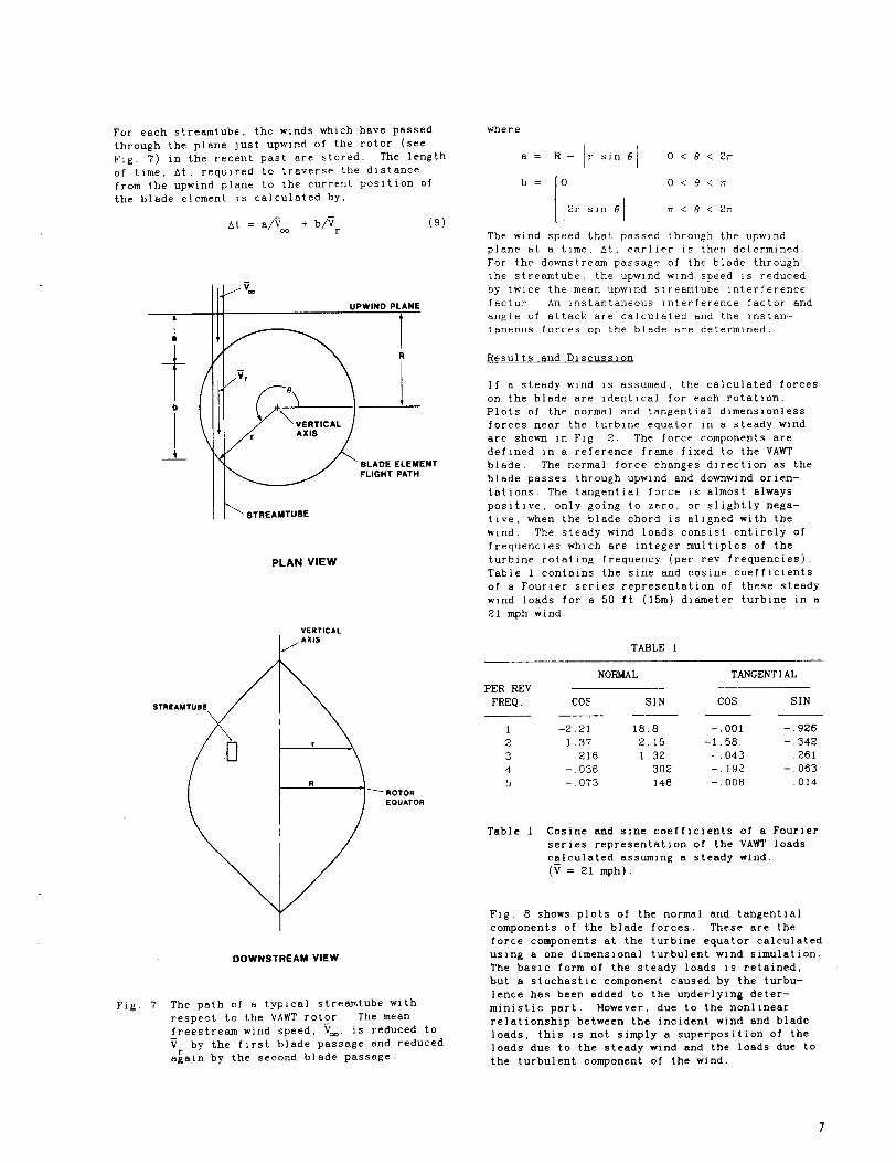
,– ––L .-L L. .._ -. ---.2 ...I.---For each Streamtube , tne wlnas wnlcn nave IJM>SCU

through the plane just upwind of the rotor (seeFig. i’) in the recent past are stored. The length

of time, At, requ]red to traverse the distancefrom the upwind plane to the current posltlon of

the blade element ]s calculated by,

(9)

V-

uPWIND PLANE

ta v

IR

b i

BLADE ELEMENTFLIGHT PATH

Ik STREAMTUSE

PLAN VIEW

VERTICAL

/AXIS

W,, c, c

a= R–rslnO 0< e < Zn

IIb=O O<e<n

2r sln .5 T< 8 < 2n

The wind speed that passed through the upwindplane at a time, At, earner ]s then determinedFor the downstream passage of the blade through

the streamtube, the upwind wind speed IS reducedby twice the mean upwind streamtube interference

factor An Instantaneous Interference factor andangle of attack are calculated and the Instan–taneous forces on the blade are determined.

Results and Dlscusslon

If a steady wind is assumed, the calculated forceson the blade are Identical for each rotation.Plots of the normal and tangential dimensionlessforces near the turbine equator In a steady windare shown in Flg 2. The force components are

defined ]n a reference frame fixed to the VAWTblade. The normal force changes direction as theblade passes through upwind and downwind orlen–

tatlons. The tangential force 1s almost alwaysposltlve, only going to zero, or sll,ghtly nega–tlve, when the blade chord 1s al)gned with thewind The steady wind loads cons]st entirely of

frequencies which are Integer multlples of theturbine rotating frequency (per rev frequencies).

Table 1 contains the sine and cosine coefficientsof a Fourier series representation of these steadywind loads for a 50 ft (15m) dlmneter turbine in a

.?1mph wind.

TABLE 1A

Fig. ‘7

STREAMTUBE

/

(h

Clr

R‘RDTOR

EOUATOR

vDOWNSTREAM VIEW

The path of a typical streemtube withrespect to the VAWT rotor. The mean

freestream wind speed, ~m, 1S reduced tO~r by the first blade passage and reduced

again by the second blade passage.

PER REVFREQ

123

45

Table 1

NORMAL TANGENTIAL

Cos SIN

–2.21 18.8

1.37 2.15216 1.32

–.036 .302

– 073 148

Cos SIN

–.001 – .926–1 .58 – .342–.043 .261

–.192 – .063

–.008 .014

Cosine and sine coefficients of a Fourierseries representation of the VAWT loadscalculated assuming a steady wind.(~= 21 mph).

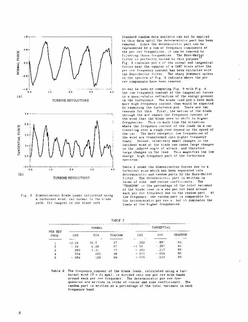
Fig. 6 shows plots of the normal and tangentialcomponents of the blade forces. These are the

force components at the turbine equator calculatedusing a one dimensional turbulent wind simulation.The basic form of the steady loads 1s retained,but a stochastic component caused by the turbu–Ience has been added to the underlying deter–ministlc part. However, due to the nonlinear

relationship between the incident wind and bladeloads, this 1s not simply a superposition of theloads due to the steady wind and the loads due tothe turbulent component of the wind.

7

-1.6I 10.0 10 20 30 40

(a)

TURBINE REVOLUTIONS

04,

I

I’A

-OIL—--------00 10 20 30 40

(b)TURBINE REVOLUTIONS

Fig. 8 Dlmenslonless Blade Loads calculated using

a turbulent w,nd, (a) normal to the bladepath, (b,) tangent. to the blade path

Standard random data analysls can not be applledto this data until the determ]nlstlc part has beenremoved S]nce the determ]nlstlc part can berepresented by a sum of frequency components at

the per rev frequencies, It can be removed byfllterlng those frequencies The Buys-Bal ~~t

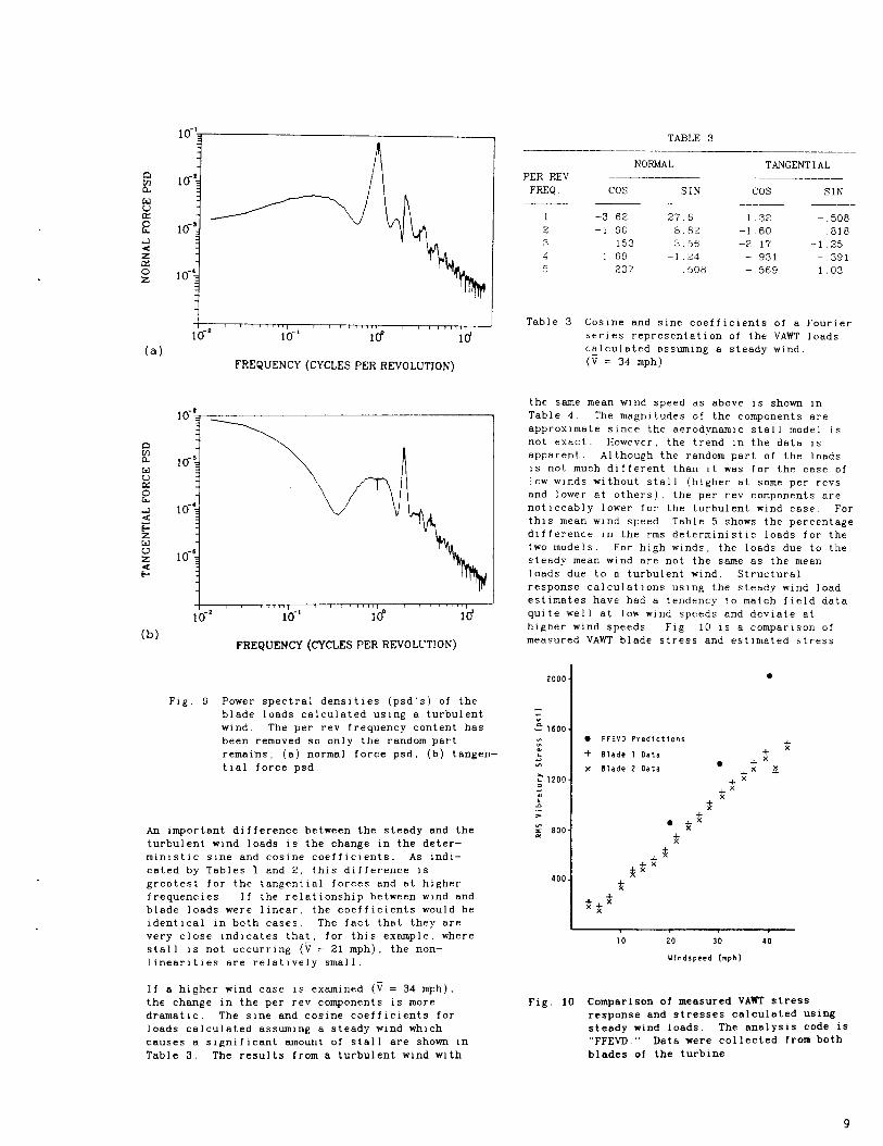
filter 1s perfectly su]ted to this purposeFig. 9 contains psd’s of the normal and tangential

forces near the equator of a VAWT blade after theper rev frequency content has been extracted with

the Buys–Ballot filter. The sharp downward spikes

In the spectra of Fig. 9 indicate where the perrev components have been removed.

As may be seen by comparing Fig. 9 with Fig. 4,

the low frequency content of the tangential forces1s a qua.s–static reflection of the energy presentIn the turbulence. The blade load psd’s have much

more high frequency content than would be expectedby examlnlng the turbulence psd. There are two

reasons for this F~rst, the motion of the blade

through the alr causes the frequency content ofthe wind that the blade sees to shift to higher

frequencies. This IS much llke the situationwhere the frequency content of the loads on a car

travellng over a rough road depend on the speed ofthe car The more energetic low frequencies of

the wind are transformed Into higher frequencyloads Second, relatively small changes in the

Incident wind at the blade can cause large changes

in the Induced angle of attack, and thereforelarge changes In the load. This magnifies the low

energy, h]gh frequency part of the turbulencespectrum

Table 2 shows the dimensionless forces due to aturbulent wind which has been separated Intodetermlnlstlc and random parts by the Buys–Ballotfilter The deterrnln]stlc part 1s written in

terms of sine and cosine coefficients. The

“ZRANDOM” IS the percentage of the total variance

of the blade load In a one per rev band aroundeach per rev frequency due to the random part. Atlow frequency, the random part 1s comparable to

the determlnlstlc per rev’s, but lt dominates the

loads at the higher frequencies.

TABLE 2

NORMAL

PER REV _———

FREQ Cos SIN ZWNDOM————— ———

1 –2.24 18.7 17

2 1 24 2 20 67

3 260 131 ?-i

4 004 .225 98.

5 – 084 .129 99.

TANGENTIAL

Cos SIN %RLNDOM—

029 – 891 69

–1 52 –.387 45

–.101 ,212 89.

– 211 – 004 90– 019 031 99

Table 2 The frequency content of the blade loads, calculated using a tur–bulent wind (~ = 21 mph), 1s dlv]ded Into one per rev wide bandsaround each per rev frequency. The determlnlstlc per rev fre–quencles are written In terms of cosine and sine coefficients. The

random part 1s written as a percentage of the total variance in eachfrequency band.

10-’

10-:

10-2

10-;

j10-2

(10-’

Ilcf

IId

mEQuENcy (CYCLESPER REVOLUTION)

I I1 1 1

10-’ 10-’ I& Id

FREQUENCY (HCLES PER REVOLUTION

Fig. 9 Power spectral dens it]es (psd’s) of theblade loads calculated using a turbulentwind The per rev frequency content hasbeen removed so only the random part

remains, (a) normal force psd, (b) tangen-tial force psd.

An Important difference between the steady and thei,urbulent wind loads 1s the change in the deter–

minlstlc sine and cosine coefficients. As indi–

cated by Tables I and 2, this difference is

greatest for the tangential forces and at higherfrequencies If the relat)onshlp between wind andblade loads were llnear, the coefficients would be

ldentlcal In both cases. The fact that they arevery close lnd]cates that, for this example, wherestall is not occurring (~ = 21 mph), the non–

IInearltles are relatively small.

If a higher wind case 1s examined (~ = 34 mph),the change In the per rev components 1s moredramatic. The sine and cosine coefficients for

loads calculated assuming a steady wind whichcauses a slgnlflcant amount of stall are shown in

l’able 3. The results from a turbulent wind with

TABLE 3— —

PER REV

FREQ

12345

Table 3

the sameTable 4.

NORMAL

Cos SIN—————

–3.62 27.6–1 90 8.82

153 3 561 69 –1 24237 .508

TANGENTIAL

Cos SIN

1.32 –.508–1.60 .816–2 17 –1.25– 931 –.391–.569 1.03

Cosine and sine coefficients of a Fourierseries representation of the VAWT loadscalculated assuming a steady wind.(~= 34mph)

mean wind speed as above 1s shown In

The magnitudes of the components are

aPPrOxlmate Since the aerodynamic stall model IS

not exact. However, the trend ]n the data ]sapparent Although the random part of the loads1s not much different than It was for the case oflow w]nds without stall (higher at some per revsand lower at others), the per rev components are

noticeably lower for the turbulent wind case, Forthis mean wind speed, Table 5 shows the percentagedifference In the rms determlnlst]c loads for the

two models For high w]nds, the loads due to thesteady mean wind are not the same as the mean

loads due to a turbulent wind. Structuralresponse calculations using the steady wind loadestimates have had a tendency to match field data

quite well at low wind speeds and deviate athigher wind speeds. F]g 10 1s a comparison ofmeasured VAWT blade stress and estimated stress

● FFIVD Predictions $+ Blade 1 Oata

● Jx Blade 2 Oata +

$~

L*

I10 20 30 40

Iifndspeed (mph)

Fig. 10 Comparison of measured VAWT stressresponse and stresses calculated usingsteady wind loads. The analysls code is

“FFEVI).” Data were collected from both

blades of the turbine.

9

response using stea~y wind Input as reported by

Lobltz and Sullivan The overpredictlon of thestress response in high winds IS consistent withthe overpredictlon of blade forces which resultsfrom assuming a steady wind.

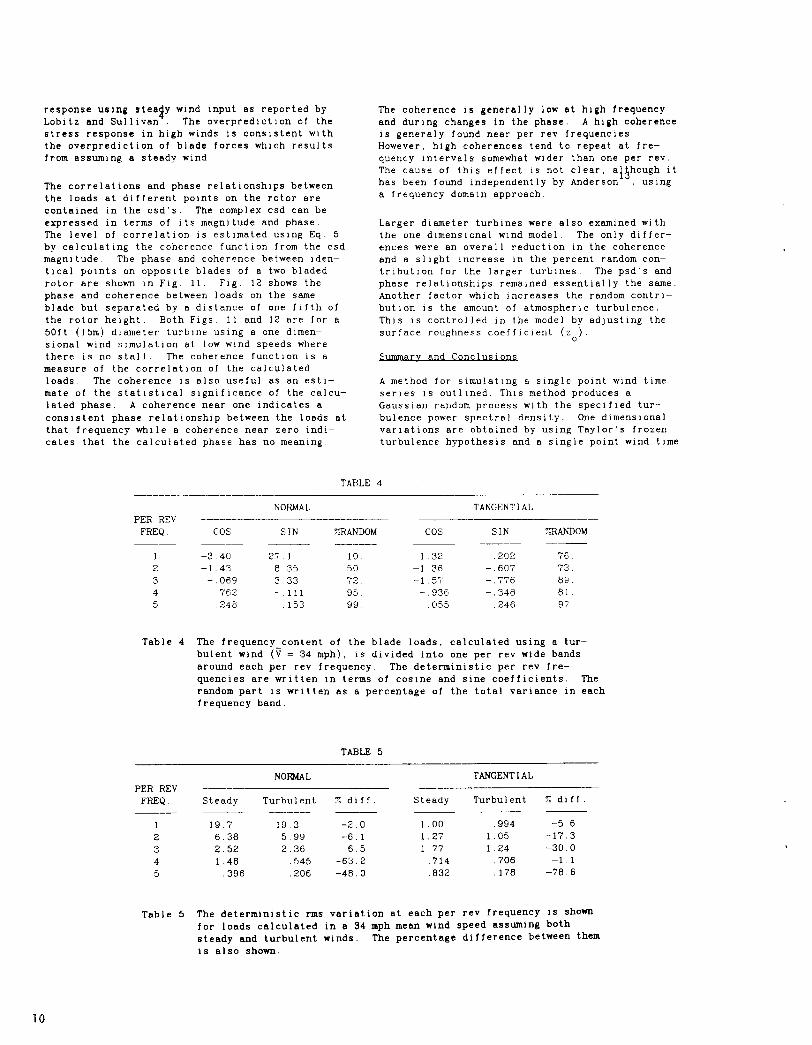
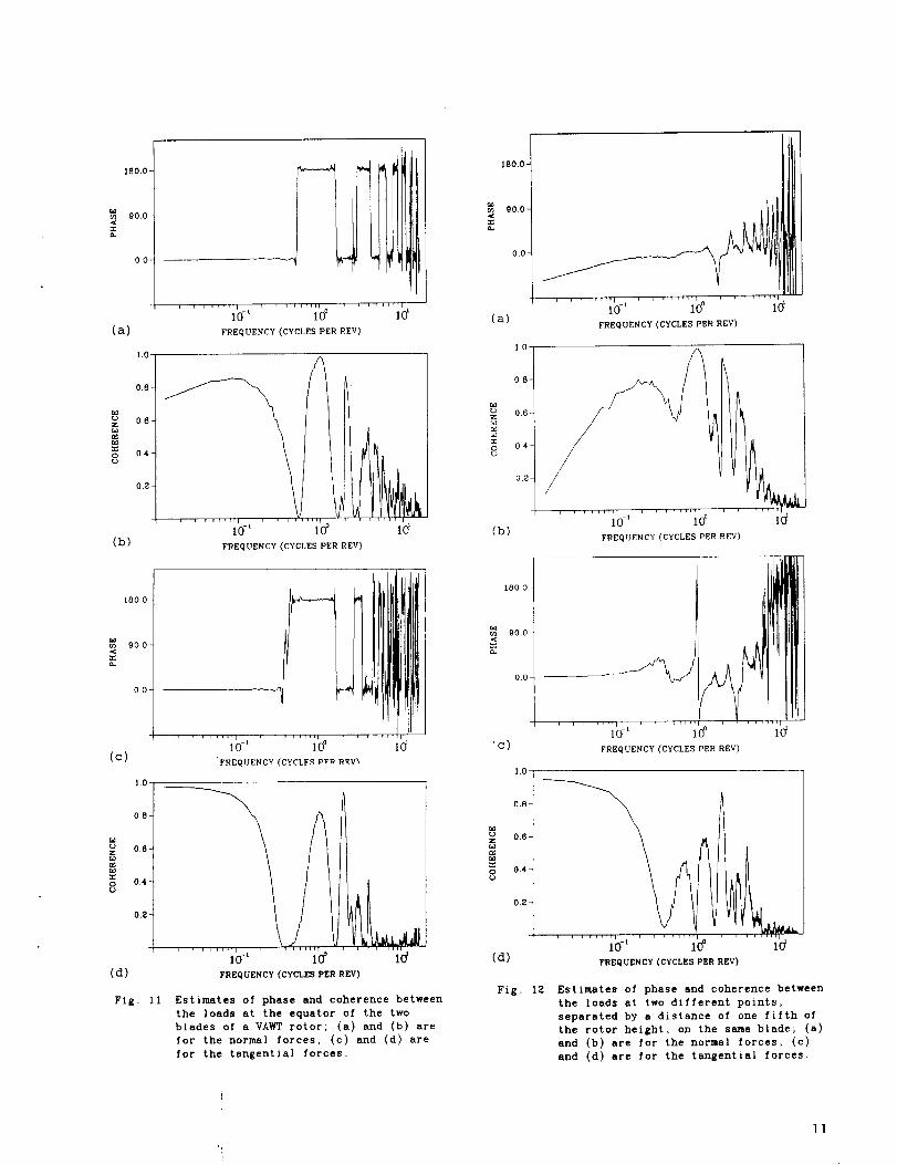
The correlations and phase relationships betweenthe loads at different points on the rotor arecontained In the csd’s. The complex csd can be

expressed in terms of its magnitude and phase.The level of correlation ]s estimated using Eq. 5by calculating the coherence function from the csdmagnitude. The phase and coherence between ]den–

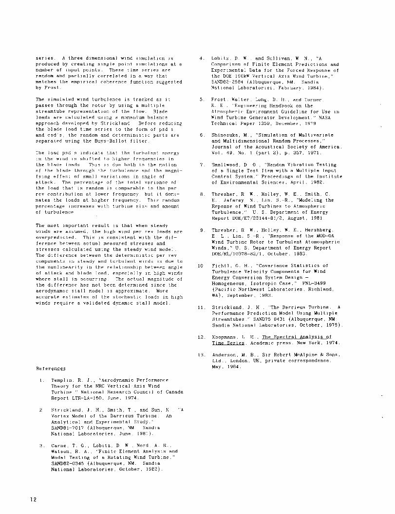
tlcal points on opposite blades of a two bladedrotor are shown in Fig. 11. Fig. 12 shows the

phase and coherence between loads on the sameblade but separated by a distance of one fifth of

the rotor height. Both Figs. 11 and 12 are for a

50ft (15m) dlemeter turbine using a one dlmen–s]onal wind simulation at low wind speeds wherethere is no stall. The coherence funct]on ls a

measure of the correlation of the calculatedloads The coherence 1s also useful as an estl–

mate of the statistical significance of the calcu–lated phase. A coherence near one Indicates a

consistent phase relat]onshlp between the loads atthat frequency while a coherence near zero indl–cates that the calculated phase has no meaning.

The coherence is generally low at high frequency

and during changes in the phase A high coherenceis generaly found near per rev frequenciesHowever, high coherence tend to repeat at fre–quency Intervals somewhat wider than one per rev.The cause of this effect IS not clear, e\\hough 1 t

has been found Independently by Anderson , usinga frequency domain approach.

Larger diameter turbines were also examined withthe one d]menslonal wind model. The only dlffer–

ences were an overall reduction in the coherenceand a sl]ght increase in the percent random con–trlbut]on for the larger turbines. The psd’ s and

phase relationships remained essentially the same.Another factor which Increases the random contri–butlon IS the amount of atmospheric turbulence.

This 1s controlled In the model by ad]ustlng thesurface roughness coeff]clent (zo).

Summarv and Conclusions

A method for simulating a single po]nt w]nd timeser]es ]s outl]ned. This method produces aGauss Ian random process with the specified tur–bulence power spectral dens]ty. One dimensionalvar]at]ons are obtained by using Taylor’s frozen

turbulence hypothesis and a single point wind time

TABLE 4

NORMAL TANGENTIALPER REV —

FREQ Cos SIN %RANOOM Cos SIN 7ZRANDOM— ——— ——

1 –3 40 z? 1 10 1.32 .202 762 –1 43 0.35 50 –1.36 – 607 ‘?3

3 –.069 3 33 ‘iZ –1.57 – 776 854 762 – 111 95 –.936 – :348 815 248 .153 99. 055 .246 97

Table 4 The frequency content of the blade loads, calculated using a tur–bulent wind (~ = 34 mph), is divided Into one per rev wide bandsaround each per rev frequency. The determlnlstlc per rev fre–quencies are written In terms of cosine and sine coefficients. Therandom part is written as a percentage of the total variance In eachfrequency band.

TABLE 5

PER REVFREQ Steady

1 19 7

2 6 38

3 2.52

4 1.48

5 .396

NORMAL TANGENTIAL

Turbulent Z dlff

19 35 992.36.545

.206

–2.0–6.1–6.5–63.2–46.0

Steady Turbulent Z dlff— —

1.00 .994 –5.6

1.27 1.05 –17.3

1.77 1.24 –30.0

.714 .706 –1 1

.632 .178 –78 .6

Table 5 The deterministic rms variation at each per rev frequency is shownfor loads calculated in a 34 mph mean wind speed assuming bothsteady and turbulent winds. The percentage difference between them

is also shown.

10

I4 1 1 1

10-’ 10° Id(a) FRi3quENcy(CYCLESPER REV)

1.0

A 1

(b)

1800

ww 90.0sn.

0,0

(c)

0.8

0.6

0,4

0.2

rREfauENcY(CYCLESpER REV)

1 1 1

10-’ 10° 10’rREqumfcY (CYCLES PFR REV)

l.o-

0,8-

0.6-

0.4-

0.2-

iwmumcy (CYCLESpER REV)

Fig. 11 Estimates of phase and coherence betweenthe loads at the equator of the twoblades of a VAWT rotor; (a) and (b) arefor the normal forces, (c) and (d) are

for the tangential forces.

180.0

q 90.0

E

0.0

(a) mmumcy (cycLEsPER REV)

10 [ A I

08

Wuz 0.6w$z0 04u

0.2

~ p, :11 :’,L

(b)10-’ 10° Id

FREQUENCY (cYcIXs PER REV)

1800

90,0

0.0

10-’ 10° 10’(c) FREQUENCY (cycLEspER REV)

0.6

0.4

0.2

~ ,,,,,,,M ,!, L

10-’ 10° ldFREQUENCY (CYCLESPER REV)

Fig. 12 Estimates of phase and coherence betweenthe loads at two different points,separated by a distance of one fifth ofthe rotor height, on the same blade; (a)

and (b) are for the normal forces, (c)

and (d) are for the tangential forces.

11

series A three dimensional wind simulation 1sproduced by creating single point s]mulatlons at anumber of Input points. These t]me series arerandom and partially correlated In a way thatmatches the emplrlcal coherence function suggestedby Frost

The simulated wind turbulence ]s tracked as ltpasses through the rotor by using a multlple

streamtube representation of the flow. B1 &deloads are calculated using a momentum balance

apprOach developed by Strickland. Before reducing

the blade load time series to the form of psd’sand csd’s, the random and determlnlst]c parts areseparated using the Buys–Ballot filter,

The load psd’s Ind]cate that the turbulent energy

In the wind ]s shifted to higher frequencies Inthe blade loads This ]s due both to the motionof the blade through the turbulence and the magnl–fylng effect of small variations In angle ofattack The percentage of the total variance of

the load that 1s random lS comparable to the perrev contr)butlon at lower frequency, but lt doml–

nates the loads at h]gher frequency. This randompercentage Increases with turbine SIZ? and amount

of turbulence

The most Important result is that when steadywinds are assumed, the high wind per rev loadsoverpredlcied. This IS consistent with the di

ference between actual measured stresses andstresses calculated using the steady w]nd mode

are

The difference between the determlnlstlc per revcomponents )n steady and turbulent winds IS due tothe nonl)nearlty In the relationship between angleof attack and blade load, especially in h]gh windswhere stall in occurring. The actual magn]tude ofthe difference has not been determined since theaerodynamic stall model 1s approximate. More

accurate estimates of the stochastic loads In highwinds require a valldated dynemlc stall model

4

5

6

7

8

9

10

11

12

13

References

1. Templln, R. J , “Aerodynamic PerformanceTheory for the NRC Vertical–Axis Wind

Turbine, ” National Research Council of Canada

Report LTR–LA–160, June, 1974.

2 Strickland, J H , Smith, T , and Sun, K “AVortex Model of the Darrleus Turbine. An

Analytical and Experimental Study,”SAND81-7017 (Albuquerque, NM Sandla

National Laboratories, June, 1981).

Lobltz. D. W., and Sulllvan, W N., “AComparison of Flnlte Element Predictions and

Experimental Data for the Forced Response ofthe DOE 100kW Vertical AXIS W]nd Turbine, ”SAND82-2584 (Albuquerque, NM. SandlaNational Laboratories, February, 1984).

Frost , Walter, Long, D. H. , and Turner,

R.E> “Englneer]ng Handbook on theAtmospheric Environment Guldellne for Use InWind Turbine Generator Development, ” NASA

Technical Paper 1359, December, 1979

Shlnozuka, M., “Simulation of Multlvarlateand Multldlmenslonal Random Processes,r’

Journal of the Acoustical Society of America,Vol. 49, No. 1 (part 2), p. 357, 1971.

Smallwood, D. O., “Random Vibration Testingof a Single Test Item with a Multlple InputControl System,” Proceedings of the Instituteof Environmental Sc]ences, April, 1982.

Thresher, R. W., Honey, W E., Smith, C.

E., Jafarey, N., Lin, S.–R., “Modellng the

Reponse of Wind Turbines to Atmospheric

Turbulence, ” U. S. Department of Energy

Report DOE/ET/23144-81/Z, August, 1961.

Thresher, R. W, , Honey, W E,, Hershberg,

E. L , Lln, S.–R., “Response of the MOD–OAWind Turbine Rotor to Turbulent Atmospheric

Winds,’< U. S. Department of Energy Report

DOE/RL/10378–82/1, October, 1983.

Flchtl> G. H., “COvariance Statistics ofTurbulence Veloclty Components for Wind

Energy Conversion System Design –Homogeneous , Isotropic Case,” PNL–3499(Paclflc Northwest Laboratories, Rlchland,WA) , September, 1983.

Strickland, J. H , “The DarrPerformance Predlctlon ModelStreamtubes,” SAND75-0431 (A

Sandla National Laboratories

eus Turbine. AUsing Multlple

buquerque, NM.October, 1975).

Koopmans, L. H. , The %ectral .knalVSIS of

Time Series, Academic press, New York, 1974.

Anderson, M. B., Slr Robert McAlplne & Sons,

Ltd. , London, UK, private correspondence,

May, 1984.

3. Carrie, T. G., Lobltz. D W., Nerd, A. R.,Watson, R. A., “F~nite Element Analysls and

Modal Testing of a Rotating Wind Turbine, ”

SAND82-0345 (Albuquerque, Nh. Sandla

National Laboratories, October, 1982).

12

DISTRIBUTION:

Aerolite, Inc.S50 Russells Mills RoadSouth Dartmouth, MA 02748Attn: R. K. St. Aubin

Alcoa Technical Center (4)Aluminum Company of AmericaAICOa Centert PA 15069Attn : D. K. Ai

J. T. HuangJ. R. JombockJ. L. Prohaska

Alternative Sources of EnergyMilaca, MN 56353Attn: Larry Stoiaken

Amarillo CollegeAmarillo, Tx -/9100Attn: E. Gilmore

American Wind Energy Association1516 King StreetAlexandria, VA 22314

Arizona state UniversityUniversity LibraryTempe, Az 85281Attn: M. E. Beecher

Atlantic wind Test SiteP.O. BOX 189Tignish P.E.I.CANADA COB 2B0Attn: R. G. Richards

Battelle-Pacific Northwest Laboratory (4)P. O. Box 999Richland, WA 99352Attn: J. R. Connell

R. L. GeorgeD. C. Powell

L. Wendell

Dr. George BergelesDept. of Mechanical EngineeringNational Technical University42, Patission StreetAthens, GREECE

Bonneville Power AdministrationP.O. BOX 3621Portland, OR 97225Attn: N. Butler

Burns & ROeJ InC.800 Kinderkamack RoadOradell, NJ 07649Attn: G. A. Fontana

California State Energy CommissionResearch and Development Division1111 HOWe Avenue

Sacramento, CA 95825

Attn: J. Lerner

Canadian Standards Association178 Rexdale Blvd.Rexdale, OntarioCANADA M9W 1R3Attn: Tom Watson

Professor V. A. L. ChasteauSchool of EngineeringUniversity of AucklandPrivate BagAuckland, NEW ZEALAND

Colorado State UniversityDept. of Civil EngineeringFort Collins, CO 80521Attn: R. N. Meroney

Commonwealth Electric co.BOX 368Vineyard Haven, MA 02568Attn: D. W. Dunham

Gale B. CurtisCurtis Associates3089 Oro Blanco DriveColorado springs, co 80917

M. M. Curvin11169 Loop RoadSoddy DalSY, TN 37379

Department of Economic Planningand Development

Barrett BuildingCheyenne, WY 82002Attn: G. N. Monsson

Otto de VriesNational Aerospace LaboratoryAnthony Fokkerweg 2Amsterdam 1017THE NETHERLANDS

DOE/ALOAlbuquerque, NM 87115Attn: G. P. Tennyson

DOE/ALOEnergy Technology Liaison OfficeNGDAlbuquerque, NM 87115Attn: capt. J. L. HanSOn, USAF

DOE Headquarters (20)Wind Energy Technology Division1000 Independence AvenueWashington, DC 20585Attn: L. V. Divone

P. Goldman

Dominion Aluminum Fabricating, Ltd. (2)3570 Hawkestone RoadMississauga, OntarioCAIVADA L5C 2V8Attn: D. Malcolm

L. Schienbein

13

J. B. DragtNederlands Energy Research Foundation (E.C.N. )Physics DepartmentWesterduinweg 3 Patten (nh)THE NETHERLANDS

Dynergy systems Corporation821 West L StreetLos BatIOSt CA 93635Attn: c. Fagundes

Iowa state UniversityAgricultural EngineeringAmes, IA 50010Attn: L. H. soderholm

JBF Scientific Corporat:2 Jewel DrlVeWilmington, MA 01887Attn: E. E. Johanson

Electric Power Research Institute (3)3412 HillView AvenuePalo Alto, CA 94304Attn: E. Demeo

F. GoodmanS. Kohan

Dr . Norman E. Farb10705 Providence DKIVeVilla park, CA 92667

Alcir de Faro OrlandoPontificia Universidade Catolica-PUC/RjMechanical Engineering DepartmentR. Marques de S. Vicente 225Rio de Janeiro, BRAZIL

FloWind Corporation (4)21414 68th Avenue SouthKent, WA 98031Attn: Herman M. Drees

S. TremouletI. E. VasR. Watson

Gates LearjetMid-Continent AirportP.o. Box 7707Wichita, KS 67277Attn : G. D. park

H. GerardinMechanical Engineering DepartmentFaculty of Sciences and EngineeringUniversity Laval-QuebecCANADA GIK 7P4

R. T. GriffithsUniversity College of SwanseaDept . of Mechanical EngineeringSingleton ParkSwansea SA2 8PPUNITED KINGDOM

Helion, Inc.Box 445Brownsville, CA 95919Attn: Jack Park, President

Institut de recherche d’Hydro-Quebec (3)1800, Montee Ste-JulieVarennes, Quebec

Canada JOL 2P0Attn: Gaston Beaulieu

Bernard Masse

lon Paraschivoiu

Room 213

on

KFilSeK Aluminum and Chemical Sales, Inc.14200 Cottage Grove AvenueDoltOn, IL 60419Attn: A. A. Hagman

Kaiser Aluminum and chemical Sales, Inc.6177 Sunol Blvd.P.O. BOX 877Pleasonton, CA 94566Attn: D. D. Doerr

Kaman Aerospace COKpOKatlOn

old Windsor RoadBloomfield, CT 06002Attn: W. BateSol

KZinSCiS State UniversityElectrical Engineering DepartmentManhattan, KS 66506Attn: Dr. G. L. Johnson

R. E. KellandThe College of Trades and TechnologyP.O. BOX 1693Prince Philip DriveSt. John’s, NewfoundlandCANADA AIC 5P7

KW Control Systems, Inc.RD#4, Box 914Csouth Plank RoadMic?dletown, NY 10940Attn: R. H. Klein

K?ilman Nagy LehoczkyCOKt Adelers GT. 300s10 2NORWAY

L. LiljidahlBuilding 005, Room 304Bare-westBeltsville, MD 20705

One LjungstromFFA, The Aeronautical Research InstituteBox 11021s-16111 BrommaSWEDEN

Massachusetts Institute of Technology (2)77 Massachusetts AvenueCambridge, MA 02139Attn: Professor N. D. Ham

W. L. Harris, Aero/Astro Dept.

14

H. s. MatsudaCompclsite Materials LaboratoryPioneering R&D LaboratoriesToray Industries, Inc.Sonoyama, Otsu, ShigaJAPAN 520

Michigan State UniversityDivision of Engineering ResearchEast Lansing, MI 48825Attn: 0. Krauss

Napier College of Commerce and TechnologyTutor Librarian, Technology FacultyColin.ton RoadEdinburgh, EH1O 5DTENGLAND

NASA Lewis Research Center (2)21000 Brookpark RoadCleveland, OH 44135Attn: D. Baldwin

J. Savino

National Rural Electric Cooperative Assn1800 Massachusetts Avenue NWWashington, DC 20036Attn: Wilson Prichett III

Natural Power, Inc.New Boston, NH 03070Attn: Leander Nichols

Northwestern UniversityDept . of Civil EngineeringEvanston, IL 60201Attn: R. A. Parmalee

Ohio state UniversityAerOrlaUtiCal and Astronautical Dept.2070 Neil AvenueColumbus, OH 43210Attn: Professor G. Gregorek

Oklahoma state universityMechanical Engineering Dept.StillWater, OK 76074Attn: D. K. McLaughlin

Oregon State university (2)Mechanical Engineering Dept.Corvallis, OR 97331Attn: W. E. Honey

R. E. Wilson

Pacific Gas & Electric3400 Crow Canyon RoadSan RamOn, CA 94583Attn: T. Hillesland

TrOel.S Friis pedersenRiso National Laboratorypostbox 49DK-4000 RoskildeDENMARK

Helge PetersenRiso National LaboratoryDK-4000 RoskildeDENMARK

The Power company, Inc.P.O. Box 221GeneSee DepOt, WI 53217Attn: A. A. Nedd

Public service Co. of New Hampshire1000 Elm StreetManchester, NH 03105Attn: D. L. C. Frederick

Public service Company of New MexicoP.O. BOX 2267Albuquerque, NM 87103Attn: M. Lechner

RANN, Inc.260 Sheridan Ave., Suite 414Palo Alto, CA 94306Attn:Alfred J. Eggers, Jr.

Chairman of the Board

Renewable Energy Ventures190 south King Street, suite 2460Honolulu, HI 96813Attn: G. W. Stricker

The Resources AgencyDepartment of Water ResourcesEnergy Division1416 9th streetP.o. BOX 388Sacramento, CA 95802Attn: R. G. Ferreira

Reynolds Metals CompanyMill Products Division6601 West Broad StreetRichmond, VA 23261Attn: G. E. Lennox

A. RobbMemorial University of NewfoundlandFaculty of Engineering and Applied SciencesSt. John’s NewfoundlandCANADA AIC 5S7

Rockwell International (2)Rocky Flats PlantP.O. BOX 464Golden, CO 80401Attn: Terry Healy

Dr . -Ing. Hans RuscheweyhInstitut fur LeichbauTechnische Hochschule AachenWullnerstrasse 7GERMANY

Beatrice de Saint LouventEstablissement d’Etudes et de Recherches

MeteorologigueS77, Rue de Serves92106 Boulogne-Billancourt cedexFRANCE

Gwen SchreinerLibrarianNational Atomic MuseumAlbuquerque, NM 87185

15

Arnan SeginerProfessor of AerodynamicsTechnion-Israel Institute of TechnologyDepartment of Aeronautical EngineeringHaifa, ISRAEL

David sharpeKingston PolytechnicCanbury Park RoadKingston, SurreyUNITED KINGDOM

Kent Smith

Instituto Technologico Costa RicoApartado 159 CartagoCOSTA RICA

Solar InitiativeCiticorp Plaza, Suite 900180 Grand AvenueOakland, CA 94612Attn: Jerry !fudelson

L, ,.:.,. SarensonRc,:,:ilde University CenterEne[gy Group, Bldg. 17.2~]:~:;~>.

?.0. BOX 260DK-400 RoskildeDENF?ARK

South Dakota School of Mines and TechnologyDept. of Mechanical EngineeringRapid City, SD 57701Attn : E. E. Anderson

Southern California EdisonResearch 6 Development Dept., Room 497P.o. BOX 800Rosemead, CA 91770Attn: R. L. Scheffler

southern Illinois UniversitySchool of EngineeringCarbondale, IL 62901Attn: C. W. Dodd

G. StaceyThe University of ReadingDepartment of EngineeringWhiteknights, Reading, RG6 2AYENGLAND

Stanford UniversityMechanical Engineering,Design DivisionStanford, CA 94305Attn : Drew Nelson

Stanford University (2)Civil Engineering DepartmentStanford, CA 94305Attn: C. A. Cornell

S. Winterstien

stanford universityDept . of Aeronautics and

Astronautics Mechanical EngineeringStanford, CA 94305Attn: Holt Ashley

R. J. Templin (3)Low speed Aerodynamics LaboratoryNRC-National Aeronautical EstablishmentMontreal RoadOttawa, Ontarior KIA 0R6CANADA

Texas Tech University (2)Mechanical Engineering Dept.P.O. BOX 4389LuDbock, TX 79409Attn: .J. W. Oler

J. Strickland

Tulane UniversityDept. of Mechanical EngineeringNew Orleans, LA 70018Attn: R. G. Watts

Tumac Industries, Inc.650 Ford StreetColorado Springs, CO 80915Attn: LJ. R. McConnell

J, M. TUrnerTerrestrial Energy Technology Program OfficeEnergy Conversion BranchAerospace Power DivisionAero Propulsion LaboratoryAir FOrCe Wright Aeronautical LaboratoriesWright-Patterson Air Force Base, OH 45433

United Engineers and Constructors, Inc.PO BoX 8223Philadelphia, PA 19101Attn: A. J. Karalis

University of AlaskaGeophysical InstituteFairbanks, AK 99701Attn: T. Wentink, Jr.

University of CaliforniaInstitute of Geophysics

and planetary physicsRiverside, CA 92521Attn: Dr. P. J. Baum

University of ColoradoDept . of Aerospace Engineering SciencesBoulder, CO 80309Attn: J. D. Fock, Jr.

University of MassachusettsMechanical anti Aerospace Engineering Dept.Amherst, MA 01003A.ttn: Dr. D. E. cromack

University of New MexicoKew Mexico Engineering Research Institutecampus P.o. Box 25Albuquerque, NM 87131Attn: G. G. Leigh

University of OklahomaAero Engineering DepartmentNorman, OK 73069Attn: K. Bergey

16

University of Sherbrooke

.Faculty of Applied ScienceSherbrooke, QuebecCANADA JIK 2Rl

Attn: R. Camerero

The University of TennesseeDept . of Electrical EngineeringKnoxville, TN 37916Attn: T. W. Recdoch

[JSDA, Agricultural Research Service:;outhwest Great Plains Research Center13ushland, TX 79012Attn: Dr. R. N. Clark

[Jtah Power and Light co.51 East Main Streetp-o. BOX 277

American Fork, UT 84003

Attn: K. R. Rasmussen

VAWTPOWER, Inc.$1733 Coors Nw

Albuquerque, NM 87114Attn: P. N. Vosburgh

Washington State UniversityDept. of Electrical Engineeringpullman, WA 99163Attn: F. K. Bechtel

WeSt Texas State UniversityGovernment Depository LibraryNumber 613Canyonr TX 79015

West Texas State UniversityDepartment of Physics~>.o, Box 248

canyon, Tx 79016Attn: V. Nelson

West Virginia UniversityDept . of Aero Engineering1.062 KOUntZ Avenue

Morgantown, WV 26505

Attn: R. Walters

D . WestlindCentral Lincoln PeOple’S Utility District2129 North Coast Highway

NeWpOrtt OR 97365-1795

Wichita State universityPieL_O Engineering Department (2)hlichita, KS 67208Attn: M. Snyder

W. Wentz

hfind Energy ReportBox 14102 S. Village AvenueRockville Centre, NY 11571A,ttn: Farrell smith Seiler

Wisconsin Division of State Energy8th Floor101 South Webster streetMadison, WI 53702Attn: Wind Program Manager

Robert AkinsProfessor of EngineeringWashington and Lee UniversityLexington, VA 24450

Dr. Michael B. AndersonSir Robert ?4cAlpine & Sons, Ltd.P. O. Box 7440 Bernard Street

London wcm lLGENGLAND

Theodore S. AndersonAdvanced Energy Systems DivisionWestinghouse Electric CorporationP. O. BOX 10864Pittsburgh, PA 15236

1520152215231523152415241524160016301633163625253141-131513154-3

316031616000620062206225622562256225622562256225622562256225711175438024

D. J. McCloskeyR. C. Reuter, Jr.J. H. BiffleD. B. ClaussD. W. LobitzP. S. Veers (25)W. N. SullivanR. G. ClemR. C. MaydewR. E. SheldahlJ. K. ColeR. P. ClarkC. M. OstranderW. L. Garner (3)C. H. Dalin (28)for DOE/TIC (Unlimited Release)J. E. Mitchell (15)P. S. WilsonE. H. BecknerV. L. DuganD. G. SchuelerR. H. Braasch (50)D. E. Berg

J. D. CyrusR. D. Grover

E. G. KadlecP. C. Klimas

M. T. NattisonR. O. NellumsD. S. OscarM. H. Worstell

J. W. ReedR. RodemanN. A. Pound

h’ind Power DigestP. O. BOX 700Bascom, OH 44809A,ttn: Michael Evans

17