8. sea-level change - florida gulf coast...

Principles of Paleoclimatology: Perspectives in Paleobiology and Earth History, by Thomas M. Cronin

8. Sea-Level Change

. . . in speculating on catastrophes by water, we certainly anticipate great floods in the future, and we may, therefore presume that they have happened again and again in past times.

Sir Charles Lyell, 1830.

By Land or By Sea?

For centuries Scandinavian naturalists have noted a remarkable phenomenon–their country’s land area was increasing and their coasts were rising. Skerries were becoming islands, waterways were closed, and submerged forests were rising. Nils-Axel Morner of Sweden (1979a) describes how in 1743, Anders Celsius, inventor of the thermometer and famed for his temperature scale, calculated a rate of coastal rise (or relative sea-level fall) of 1.2 cm/yr along Swedish coasts. The rising land gave considerable support to the eighteenth-century theory of Neptunism, which held that sea level was continuously falling in a one-way direction. Indeed, this trend of falling sea level continues today in Scandinavia at a rate of 1–2 cm/yr.

On Smith Island, located in the heart of Chesapeake Bay, the opposite has been happening. When English colonists settled in the seventeenth century, Smith Island was ideal for grazing cattle, and bay waters off its shores were bountiful with finfish and shellfish. Over the past three centuries, however, its coasts, like those of other Chesapeake Bay islands, have suffered from severe erosion and shoreline retreat. Smith Island has been reduced in area from 11,000 acres in 1849 and to 7000 acres of mostly marshland by the 1980s. Tide gauges, first established in the Chesapeake and its tributaries in Baltimore (1903), Annapolis (1929), and Solomon (1938), Maryland, as well as Washington, D.C. (1931), record vertical coastal submergence at rates between 3.17 and 3.56 mm/yr (Hicks and Hickman 1988; Emery and Aubrey 1991). In a century, this amounts to more than a 30-cm sea-level rise relative to the land surface. Coasts along Chesapeake Bay are retreating in a linear direction as well. Dolan et al. (1983) concluded that the average rate of retreat of Chesapeake Bay coastlines was 0.7 m/yr, a rate much higher than that of other coasts of the United States.

The Chenier Plain and Mississippi Delta of the Louisiana coast, a complex nexus of swamps, fresh and saltwater

marshes, alluvial plains, and barrier islands, is another region undergoing coastal submergence. About 3950 km2 of Louisiana coastal wetlands–a region the size of the state of Rhode Island–have been lost between 1930 and 1990. Louisiana has 40% of the total wetlands in the United States and has suffered 80% of the nation’s wetland loss over the past century. As a result, concern about future coastal land loss in Louisiana and elsewhere has become a national priority (Boesch et al. 1994).

What factors are causing Sweden’s coasts to rise, Chesapeake Bay islands to shrink, and Louisiana coastal wetlands to disappear? Can the much-publicized global sea-level rise account for coastal submergence in Chesapeake Bay and in Louisiana, and a sea-level fall in Scandinavia simultaneously? In previous chapters the topic of sea-level change was described with reference to several subtopics of paleoclimatology: emerged coral terraces and the orbital theory of climate change, low sea level during the last glacial maximum (LGM), and glacial meltwater that caused sea level to rise during deglaciation. In this chapter, I focus on the broader topic of sea-level change and the multiple factors that complicate efforts to understand sea-level history and its intimate relationship with climate change.

Four important themes permeate sea-level and climate change and coastal evolution. First, a clear distinction must be made between the concepts of eustatic and relative sea-level change. The concept of eustatic, or global, sea-level change is credited to Austria’s Eduard Suess (1885–1909), who theorized that worldwide ocean-level

of 30Principles of Paleoclimatology

6/28/2009http://www.earthscape.org/r3/cronin/cronin08.html

changes caused observed changes in sea level. Eustatic changes in ocean level are sometimes informally referred to as absolute or global sea-level changes. Today researchers attribute eustatic sea-level variability to three major processes: steric expansion (or contraction) of upper ocean layers due to temperature and density changes; glacio-eustasy, the growth and decay of ice sheets and glaciers and concomitant volumetric changes in the world’s ocean water; and tectono-eustasy, changes in ocean basin volume (table 8-1).

Table 8-1. Some Factors Producing Observed Sea-Level Change and Their Approximate Time Scales

Geologists also recognize, however, that observed sea-level change along a coastal region is a manifestation of both eustatic sea-level change and other processes that cause the land to rise or fall. Observed changes in sea level for any particular region are therefore referred to as relative sea-level changes, and the sea-level history for that region is called a relative sea-level curve. The most important processes that affect relative sea-level records include geoidal factors (spatial and temporal variability in gravitational effect on the ocean surface), coastal subsidence or uplift due to sediment compaction or ground-water removal, local and regional tectonic uplift or subsidence, and isostatic processes related to sedimentation and erosion, hydro-isostasy, and glacio-isostasy (table 8-1). Although a eustatic sea-level rise may occur as a global and nearly synchronous event, completely separating the eustatic component of a relative sea-level curve from those parts caused by local and regional factors is difficult if not impossible. Historical coastal changes in Scandinavia, Chesapeake Bay, and Louisiana serve as textbook examples of how coastal processes act in concert with changing ocean level to affect observed trends in relative sea level. Consequently most researchers abide by the maxim, there is no single “eustatic” sea-level curve. To successfully attribute causes to any observed sea-level change, it is necessary first to decouple the effects of land-based processes like subsidence and uplift from those related to changes in ice or ocean-basin

Processes Time Scale (yr) Comments

“Absolute” or eustatic sea-level change

Steric expansion and contraction Glacio-eustasy

1–100

Alpine glacial growth and melting

10–1000 Faster response to forcing than ice sheets; glacial surges extremely rapid

Ice-sheet growth 1000–1,000,000

Stepwise growth toward full glacial interval

Ice-sheet decay 100–10,000 Rapid ice-sheet decay under some conditions

Tectono-eustasy 100,000–10,000,000

Ocean-volume changes

Relative sea-level change

Ocean dynamic processes

1–10 Kelvin and Rossby waves

Geoidal changes 1–100 Gravitational variation

Subsidence and uplift 100–10,000,000

Regionally variable; depends on sedimentation tectonics and local geology

Tectonic uplift and subsidence

<1–1,000,000 Regionally variable; coseismic vertical movements most rapid

Isostatic processes

Sedimentation and erosion

1000– > 10,000 Accumulation and removal of ediment loads

Hydro-isostasy 1000– > 10,000 ocean basin sinking lags behind ice-sheet melting

Glacio-isostasy 1000– > 10,000 Slow restoration to gravitational equilibrium after deglaciation due to high mantle viscosity



volume.

A second aspect of sea-level and climatic change is the concept that large-scale ice-volume change, the major cause of eustatic sea-level oscillations over tens of thousands of years, is itself an active agent of climate change. As discussed in earlier chapters, the areal and volumetric extent of continental and sea-ice volume influence planetary albedo, atmospheric circulation, oceanic salinity and temperature, and biogeochemical cycling in the oceans. In the example of the postglacial 125-m sea-level rise between 20 and 5 ka, this inundation of the world’s continental shelves affected ocean-margin sedimentation, upwelling, biological productivity, and nutrient budgets, ultimately influencing earth’s global elemental cycling and climate.

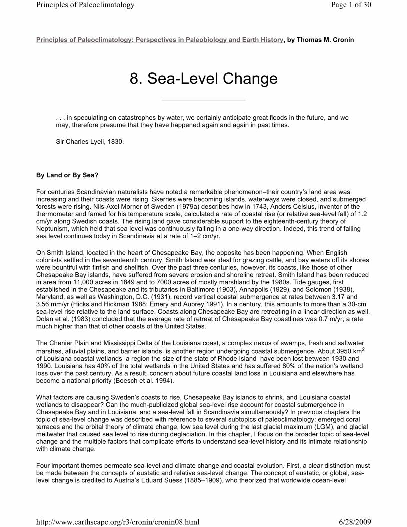
Third, all modern coastlines–whether barrier islands, coral reefs, mangroves, estuaries, deltas, or glaciated fjords–have one feature in common. Their geomorphology, sedimentology, and ecology, to varying degrees, have been influenced by postglacial sea-level rise and the redistribution of load from continental ice sheets to ocean basins. In tropical regions, notches forming overhanging cliffs testify to Holocene erosion of emerged reefs that formed during previous high stands of sea level (figure 8-1). In estuaries like Chesapeake Bay, drowned river valleys such as the ancient Susquehanna River became flooded during postglacial sea-level rise (Colman and Mixon 1987). Postglacial sea-level change left its mark on the terrestrial fauna and flora of many islands, especially in shallow marginal seas like those around Indonesia, where islands harbor terrestrial species that migrated across land bridges connecting them when sea level was lower. One striking example of mammalian migration during low sea level and subsequent isolation was the crossing of the Bering Land Bridge by Homo sapiens at least by 12 ka, just before the rapid sea-level rise that inundated the Bering Strait region.

Figure 8-1 Exposed coral-reef terrace along the coast in the city of Santo Domingo, Dominican Republic, corresponding to marine isotope stage 5e. Region is relatively stable tectonic area such that the fossil reef’s elevation about 3–4 m above modern sea level represents high global eustatic sea level during the past interglacial period, about 135–120 ka.

Finally, we must distinguish between sea-level change and coastal land loss due to processes unrelated to either relative or absolute sea-level rise or fall. Wave and storm erosion, coastal ocean currents, storm surges, changes in sediment budget (i.e., variations in sand supply), local geology (slope failure and landslides), local climate (temperature and precipitation) and vegetation are processes that affect coastal zones (Pilkey et al. 1989; Fletcher 1992). Natural processes are often exacerbated by human activities such as construction of jetties, groins, or channels; the extraction of oil, water, or gas; and irrigation and land-use changes (Jelgersma 1996). Experts believe, for example, that near Grand Isle, Louisiana, a relative sea-level rise of about 1 cm/yr accounts for only a fraction of the total coastal land loss. The remainder is attributed to other factors related to land-use practices (Boesch 1994). Others disagree as to the effects of anthropogenic factors. Whereas Sahagian et al. (1994) estimate that global sea level rose 0.54 mm/yr owing to groundwater mining, wetland drainage, deforestation, and impoundment of freshwater by dams, Gornitz et al. (1994) contend that the total anthropogenic contribution to sea-level rise over the past 60 years due to these processes and irrigation was a net fall in sea level of 1.63 mm/yr. We will not discuss coastal processes or anthropogenic activity causing coastal change further, except to note that they may contribute to and/or accelerate the impact of naturally occurring sea-level change. Many authors discuss the combined effects of coastal processes and sea level to explain regional sea-level trends (e.g., Milliman and Haq



1996).

After a brief section on early concepts of sea-level change, this chapter presents sections on geological evidence for sea-level change; the major processes that cause eustatic and relative sea-level change; Cenozoic, late Quaternary and Holocene sea-level history; and historical sea-level change of the past century.

Early Concepts of Sea-Level Change

Pre–twentieth century theories to explain sea-level changes have a long and diverse history closely linked with theories about the earth. Some of these are described in engaging books entitled Eustasy: The Historical Ups and Downs of a Major Geological Concept, edited by Robert H. Dott, Jr. (1992); Sea Levels, Land Levels and Tide Gauges, by K. O. Emery and David Aubrey (1991); and Phanerozoic Sea-Level Changes, written by Anthony Hallam (1992). Generations of leading scientists have tackled the still perplexing problem of the nature and causes of sea-level change, and it is judicious to mention a few notable examples. Early ideas that sea level was not stable came from evidence derived from marine fossils preserved in sediments exposed far above modern sea level and from observations of emerging and submerging modern coastlines. Many early interpretations of marine fossils and sea-level change were also deeply rooted in theology. For example, evidence for changing sea level was considered to be a sign of the biblical Noachian flood, a theory advocated by early seventeenth Natural Theologists such as Thomas Burnet (see Gould 1987; Dott 1992).

In the early 1800s, the Diluvialist, Catastrophist, and Neptunist schools of science also used varying lines of evidence for catastrophic submergence of the land by the ocean to support their theories. Diluvial is a term coined by William Buckland (1823) to explain superficial gravel deposits that he attributed to a great catastrophic flood. Buckland’s diluvial period of relatively high sea level had been preceded by a long “antediluvial” geological era of lower sea level and a “postdiluvial” (or alluvial) period succeeding it.

Georges Cuvier promoted the theory of Catastrophism to account for the alternating series of fossiliferous marine and nonmarine sedimentary strata and the extinction of fossil species in the Paris Basin, France. Cuvier saw relative sea-level changes that were induced by catastrophic floods. Each flood, Cuvier thought, was caused by an inversion of the sea floor, an idea that led to the “sea-floor inversion” theory of eustasy (Dott 1992).

Neptunism is a school of thought traced to the seventeenth-century work of France’s Benoit de Maillet (Carozzi 1992). Carozzi (1992:19) summarizes de Maillet’s Neptunist ideas as follows: “The present-day diminution of the sea, as inferred by de Maillet, on the earth’s surface is the sea-level fall episode of an eternally repeated cosmic and complete eustatic cycle produced by a complex interchange of water and ashes between celestial bodies within and between the various vortices.” In eighteenth-century Scotland, James Hutton, and later Abraham Gottlob Werner at Freiberg in Saxony, among others, fostered various versions of Neptunism (see Berggren 1998; Strahler 1987; Dott 1992), which flourished in the early nineteenth century. Dott (1992:3) characterized Neptunism as signifying “one-way eustatic fall of sea level.” Thus according to Dott, Neptunism explained the prevalence of marine fossiliferous strata exposed on land and the rising coastlines of Scandinavia as evidence for vertical uplift by the land rather than changes in the level of the oceans.

During the nineteenth century, Charles Lyell also held as a basic tenet of his Uniformitarian view of earth history that gradual uplift and subsidence of the land was a preferred mechanism to explain sea-level changes. Lyell believed that the mechanism he found so prevalent in many parts of the modern earth–volcanic activity–was the major cause of observed changes in ocean level evident from fossil marine organisms now found far from modern oceans. Citing the work of early naturalists of the seventeenth and eighteenth centuries, as well as his own observations, Lyell postulated that volcanic activity had displaced large land areas either upward or downward relative to the level of the sea. Lyell also strongly favored a theory of glacial drift to explain the existence of diluvium and glacial erratic boulders as the result of icebergs “drifting” into a region rather than the product of continental ice-sheet movement.

As we saw in chapter 4, the glacial theory of Louis Agassiz, which he developed in the mid-nineteenth century to explain glacial geomorphic features and sediments, was instrumental in the development of the orbital theory of climate change. Agassiz’s glacial theory also revolutionized the study of sea-level change by providing a new mechanism–continental ice-sheet growth and decay–to explain the existence of glacial features and to account for large-scale, rapid sea-level changes. With the general acceptance of Agassiz’s theory during the latter part of the



nineteenth century, glaciology and glacial geology became intricate parts of research on glacio-eustatic sea-level history. As I discuss below, glacio-eustasy is the dominant factor in explanations of large-scale (50–100 m), rapid (< 100 ka) sea-level changes occurring during late Cenozoic glacial-interglacial transition.

In sum, the earliest notions about the possibility of sea-level change emanated from the same types of evidence–rising land surfaces, fossiliferous sediments, and glacial deposits–that are still used now, as we describe in the next section.

Geological, Geochemical, Geophysical, and Biological Evidence for Sea-Level Change

We can divide the types of evidence for sea-level change into four categories: geological, geochemical, geophysical, and biological. Geological evidence comes from two broad subfields: geomorphology and stratigraphy. Geomorphological evidence for ancient shorelines that now lie either above or below present sea level is plentiful along coastal regions. Wave-cut escarpments, relict barrier islands, and fossil coral reefs are three such features. Stratigraphic evidence for sea-level oscillations occurring over various time scales include data derived from sedimentary sequences showing multiple marine transgressive and regressive episodes, punctuated by either subaeriel erosion or nonmarine deposition.

Geochemical evidence comes mainly from the stable oxygen isotopic record of deep-sea benthic and planktic foraminifers described in chapter 2. Oxygen-isotope variability, which is a function of global ice volume and other factors such as oceanic temperature and salinity and the vital effects of foraminiferal species, has been applied primarily in research on orbital-scale sea-level variability (see chapter 4).

Geophysical evidence stems mainly from two widely divergent subfields: seismic stratigraphy (Vail et al. 1977; Haq et al. 1987, 1988) and geophysical modeling of earth’s isostatic response to glacial ice-sheet growth and decay (Peltier 1993, 1994). Seismic stratigraphy uses the distinct seismic signatures of different types of sedimentary deposits and their bounding unconformities, supplemented by geochronological methods of biostratigraphy and magnetostratigraphy, to detect transgressive and regressive sedimentary sequences of continental margins (also called onlap-offlap sequences). Transgressive-regressive sedimentary sequences are believed by many to result largely from eustatic sea-level changes and regional tectonic and sedimentary processes. Seismic stratigraphy has been the major impetus behind the development of a chronostratigraphic eustatic framework, often referred to as a eustatic sea-level curve, for much of the Mesozoic and Cenozoic (Haq et al. 1987, 1988, see below).

Geophysical research on earth’s crustal and mantle rheology and deformation also plays an important role in sea-level research. A global model of “paleotopography” heavily dependent on radiocarbon-dated late Quaternary sea-level curves known as the ICE-4 model was developed by Richard Peltier to test models of earth’s crustal properties and examine global sea level and isostatic motions over the past 20 ka. Peltier’s models of glacio-eustatic sea-level change and accompanying crustal isostatic response to deglacial unloading of ice sheets contributes heavily to interpreting late Quaternary relative sea-level curves.

Biological evidence for sea-level change comes from a wide variety of organisms that today live at or near sea level, whose fossil record helps to establish the location of ancient coastal zones. The overarching principle in the reconstruction of relative sea-level history from biological evidence is as follows: the more a species’ ecological tolerances restrict its range to within the intertidal or shallow subtidal zones, the more suited it is as an indicator of past sea level. In the book entitled Sea-Level Research: A Manual for the Collection and Evaluation of Data, edited by Orson van de Plassche (1986), experts on various biological groups devote entire chapters to marine mollusks, corals, coralline algae, gastropods, buried forests, botanical macrofossils, foraminifers, ostracodes, diatoms, and even human-constructed shell middens to describe the rich array of biological evidence available to scientists conducting sea-level research. Among the best sea-level indicators are tidal marsh grasses (Spartina alterniflora), corals (Acropora palmata), mollusks (Crassostrea virginica), and benthic marsh foraminifera (Trochammina), among others. As with other biological indicators of climate-related phenomena, our knowledge of sea-level history rests on biological principles just as much as it does on the physics of glaciers or the earth’s crust.



Figure 8-2 Tide-gauge record of relative sea-level changes of the past century along coastal regions having different isostatic and tectonic processes. Courtesy of World Meteorological Association.

Finally, tide gauges are means to examine historical trends in sea level extending back about a century (figure 8-2). Tide-gauge measurements of sea level are, however, complicated not only by tectonic and isostatic factors that cause vertical motions of the land surface, but also by piling up of water due to prevailing winds and ocean currents, changes in instrumental procedures, and other factors. Emery and Aubrey (1991:162) conducted the most thorough assessment of the value of tide-gauge records as a measure of global sea level and came to the following conclusion:

We can find no justification for using a few long-term tide-gauge stations as representative for regional or global averages. The longer term data appear anomalous compared to the better regional and global estimates derived from more but shorter term data. Although the reasons for this anomaly are only hypothesized here, it appears that the long-term station data prior to about 1930 cannot be used to evaluate changes in rates of eustatic sea-level rise.



In the following section on processes affecting sea level, we will see that each particular type of evidence plays an important role in the study of sea-level history.

Processes Affecting Sea-Level Change

Scientists recognize several major processes that cause eustatic and relative sea-level changes over different time scales (table 8-1). The most important are steric changes (ocean expansion due to atmospheric and near surface oceanic warming), glacio-eustasy (sea-level rise and fall due to melting and growth of glaciers and ice sheets on land), tectono-eustasy (continental plate motions leading to ocean-ridge volume and global sea-level changes manifested in marine transgressions and regressions), ocean dynamic factors (i.e., Rossby and Kelvin waves), geoidal changes, local coastal subsidence and uplift (sediment accumulation and removal) and tectonics, and isostasy (including glacio-isostasy and hydro-isostasy, vertical crustal motions due to gravitational effects of load redistribution of glacial ice and meltwater in the oceans). The following sections summarize each of these as they pertain to coastal processes and sea-level variability (e.g., Nummendal et al. 1987; Morner 1979b; Cronin 1982; Tooley and Shennan 1987; Pirazzoli 1991; Peltier 1993; Fletcher 1992; Fletcher and Wehmiller 1992; Milliman and Haq 1996).

Eustatic Sea-Level Change

The concept of eustasy was formally introduced by Suess (1885–1909), who theorized that changes in sea level were due to global changes in the level of the world’s oceans. Suess attributed subsidence of the crust to the cooling and shrinking of the earth, causing sea level to fall, and the continuous deposition of sediments into oceans, causing sea level to rise. In the ensuing century, parallel theories were developed by Chamberlin (1898, 1916), Stille (1924), Umbgrove (1939), Graubau (1940), and other geologists in Europe and North America to account for cyclic stratigraphic sequences on the world’s continents (see Dott 1992; Hallam 1992).

Eventually, Suess’s idea that sedimentation led to global sea-level rise was discarded because marine geological and stratigraphic investigations (Hallam 1963) showed it was too minor to cause sea-level to rise and fall the > 100 m observed in stratigraphic and geologic records. Instead, ocean volume changes associated with plate tectonic theory became, and remain today, the preferred mechanism to explain first-order and perhaps second-order sea-level cycles over tens of millions of years. Eustatic sea-level changes are viewed today as resulting mainly from three types of processes: steric (thermal) effects, glacio-eustasy, and tectono-eustasy.

Steric Effects–Thermal Expansion of Oceans

Steric height, a term used in oceanography, is defined as the vertical distance (i.e., depth) between two surfaces of constant pressure. This measure is used by oceanographers to account for density differences in the oceans. The main steric effect causing eustatic sea-level change is believed to be temperature change in upper ocean layers. During the past century, steric sea-level rise is believed to have been caused by increasing atmospheric temperatures because higher temperatures warm the world’s sea-surface waters and decrease their density, causing the ocean to expand (Wigley and Raper 1987). In one study, Nerem (1995) concluded from satellite data that the global mean rate of sea-level rise was 4–6 mm/yr. This rate is higher than rates calculated from post-1900 tide-gauge records (Emery and Aubrey 1991). Nerem computed that an estimated 6- to 9-cm rise in sea level

would accompany a 1oC increase in sea surface warming. This estimate suggests that about one half of the total historical 10- to 25-cm sea-level rise of the past century was due to thermal expansion of the ocean surface. However, there is considerable uncertainty in this estimate. One source of uncertainty lies in measuring the depth below the ocean surface that is warmed. In one study of 42-yr records of ocean temperatures off coastal California,

Roemmich (1992) found a temperature increase of 0.8oC in the uppermost 100 m and smaller but significant warming as deep as 300 m. Roemmich concluded that steric expansion could account for anywhere between 30% and 100% of the observed sea-level rise from adjacent California tide-gauge records (corrected for isostatic adjustment). He emphasized, however, that because spatial and temporal variability in steric oceanic effects over decadal time scales are poorly documented, the Pacific trends cannot be extrapolated to other oceanic regions.

Despite these uncertainties, current estimates of the contribution of steric effects to sea-level rise of the past century, as determined by based on observational and modeling studies, is generally estimated at about 2–6 cm, with a best estimate of 3.5–3.8 cm (Meier 1993; Warrick and Oerlemans 1990; de Wolde et al. 1995; Cubasch et al. 1995; Warrick et al. 1996). These measures are equivalent to a rate of sea-level rise between 0.2 and 0.6



mm/yr, which roughly matches that expected from oceanic warming of 0.07oC/yr. Estimates from modeling studies depend primarily on estimates of atmospheric temperature rise, while those based on tide-gauge records depend on the length of tide-gauge records selected. The remaining portion of the historical sea-level rise most likely results from melting of alpine glaciers (Meier 1984, 1993). Unknown contributions include meltwater Antarctica and Greenland (see later) and possibly anthropogenic factors such as groundwater mining, deforestation, wetland loss, creation of reservoirs, and irrigation (Gornitz et al. 1994).

Glacio-eustasy

Glacio-eustasy refers to the theory that the melting and growth of large continental ice sheets are the cause of observed sea-level changes over 10 ka to 1 Ma. To fully appreciate the concept of glacio-eustasy and how difficult it is to determine sea-level history due to the growth and melting of glaciers, we must first review the earth’s cryosphere and the processes governing glacial and ice-sheet behavior.

Earth’s Modern Cryosphere

Although the existence of an ice-covered continent was known in the early nineteenth century, it was not until early twentieth-century expeditions to Antarctica by Ernest Shackleton, Robert Scott, and Roald Amundsen did naturalists begin to unlock the mysteries of the immense quantity of ice stored on this unexplored continent. Ironically, by the time of early Antarctic explorations, European and North American scientists already knew as much or more about the late Pleistocene ice sheets that covered Europe and North America than about the scope and history of the modern Antarctic Ice Sheet. Indeed, Maclaren (1842) and later Penck (1882) had already postulated a drop in global sea level of about 100 m due to formation of the late Pleistocene ice sheets, a figure remarkably close to modern estimates of 125 m.

The earth’s modern cryosphere–that part of the global water budget stored in ice–is a dynamic and critical part of the entire climate system (figure 8-3). As discussed in chapter 2, Antarctica holds 60% of the world’s fresh water

and 91% of its ice, an equivalent to 13.9 x 106 km2 in area and 30.1 x 106 km3 in volume. Melting of the grounded ice portion of the Antarctic Ice Sheet would cause sea level to rise about 73 m; melting of the Greenland Ice Sheet would raise sea level an estimated 7.4 m; and the world’s mountain glaciers and small ice caps would cause a sea-level rise of 0.3 m.

Processes Governing Budgets of Ice Sheets and Glaciers

At any one time, an ice sheet or a glacier has either a positive or negative mass balance depending on whether it is growing or melting. Multiple factors govern the mass balance of an ice sheet or a glacier and thus how it will affect eustatic sea level. These factors include basal melting, subglacial lithology and glacial till distribution, oceanic temperatures surrounding the margins of an ice sheet, the position of sea level with respect to grounded marine-based ice sheets, summer ablation, winter snow accumulation, ice-stream behavior, and long-term equilibrium factors related to the past deglaciation.



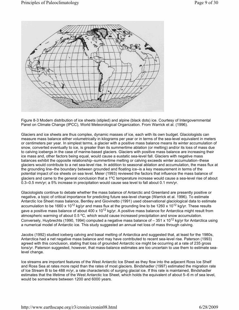
Figure 8-3 Modern distribution of ice sheets (stipled) and alpine (black dots) ice. Courtesy of Intergovernmental Panel on Climate Change (IPCC), World Meteorological Organization. From Warrick et al. (1996).

Glaciers and ice sheets are thus complex, dynamic masses of ice, each with its own budget. Glaciologists can measure mass balance either volumetrically in kilograms per year or in terms of the sea-level equivalent in meters or centimeters per year. In simplest terms, a glacier with a positive mass balance means its winter accumulation of snow, converted eventually to ice, is greater than its summertime ablation (or melting) and/or its loss of mass due to calving icebergs in the case of marine-based glaciers. Glaciers with positive mass balance are increasing their ice mass and, other factors being equal, would cause a eustatic sea-level fall. Glaciers with negative mass balances exhibit the opposite relationship–summertime melting or calving exceeds winter accumulation–these glaciers would contribute to a net sea-level rise. In addition to seasonal ablation and accumulation, the mass flux at the grounding line–the boundary between grounded and floating ice–is a key measurement in terms of the potential impact of ice sheets on sea level. Meier (1993) reviewed the factors that influence the mass balance of

glaciers and came to the general conclusion that a 1oC temperature increase would cause a sea-level rise of about 0.3–0.5 mm/yr; a 5% increase in precipitation would cause sea level to fall about 0.1 mm/yr.

Glaciologists continue to debate whether the mass balance of Antarctic and Greenland are presently positive or negative, a topic of critical importance for predicting future sea-level change (Warrick et al. 1996). To estimate Antarctic Ice Sheet mass balance, Bentley and Giovinetto (1991) used observational glaciological data to estimate

accumulation to be 1660 x 1012 kg/yr and mass flux at the grounding line to be 1260 x 1012 kg/yr. These results

gave a positive mass balance of about 400 x 1012 kg/yr. A positive mass balance for Antarctica might result from

atmospheric warming of about 0.5 oC, which would cause increased precipitation and snow accumulation.

Conversely, Huybrechts (1990, 1994) computed a negative mass balance of – 351 x 1012 kg/yr for Antarctica using a numerical model of Antarctic ice. This study suggested an annual net loss of mass through calving.

Jacobs (1992) studied iceberg calving and basal melting of Antarctica and suggested that, at least for the 1980s, Antarctica had a net negative mass balance and may have contributed to recent sea-level rise. Paterson (1993) agreed with this conclusion, stating that loss of grounded Antarctic ice might be occurring at a rate of 235 gross tons/yr. Paterson suggested, however, that mass-balance estimates are too uncertain to use them to estimate sea-level change.

Ice streams are important features of the West Antarctic Ice Sheet as they flow into the adjacent Ross Ice Shelf and Ross Sea at rates more rapid than the rates of most glaciers. Bindshadler (1997) estimated the migration rate of Ice Stream B to be 488 m/yr, a rate characteristic of surging glacial ice. If this rate is maintained, Bindshadler estimates that the lifetime of the West Antarctic Ice Sheet, which holds the equivalent of about 5–6 m of sea level, would be somewhere between 1200 and 6000 years.



The mass balance of Greenland over the past century is also unclear (see Meier 1993; Paterson 1993). Zwally et al. (1989) used satellite data from 1978–1986 to show the equivalent ice growth of 0.45 ± 0.25 mm/yr. Budd and Smith (1985) and Fortuin and Oerlemans (1990) also suggested Greenland has a positive mass balance and thus contributes to a lowering of the net historical sea-level trend. A review of ongoing research on Greenland and Antarctic Ice Sheet behavior is beyond the scope of this chapter, but major improvements in understanding the mass balance of different segments can be anticipated in the near future.

Small glaciers and ice caps also contribute to sea-level change. Meier (1984, 1993) and Trupin et al. (1992) used monitoring data from dozens of glaciers from 31 regions of the world to provide a range of estimates of 0.18–0.46 mm/yr for the sea-level rise during the past century due to melting of small glaciers and ice caps. However, most of their data came from Northern Hemisphere glaciers, and additional work is needed. Warrick et al. (1996) estimated that sea level rose 0.60 mm/yr owing to small glacier melting for the period 1985–1993. As we saw in chapter 6 in reference to climate change since the Little Ice Age, historical records indeed show that small glaciers have been receding around the world during the past century, and estimates suggest that they have contributed between 5 and 15 cm to the total sea-level rise since the late nineteenth century.

Paterson (1993) summarized available evidence for the contribution that modern ice sheets and glaciers make to the total 1.8 mm/yr sea-level rise of the past century as follows: smaller glaciers, about 0.46 ± 0.26 mm/yr; Greenland Ice Sheet, about 0.29 ± 0.15 mm/yr; Antarctica, about 0.65 ± 0.61 mm/yr. The remaining 0.4 ± 0.2 mm/yr was due to thermal expansion of the oceans.

To summarize, although significant progress has been made in glaciology, determining the glacio-eustatic contribution to the past century’s sea-level rise has a large degree of uncertainty (1.2 mm/yr ± 0.6 mm/yr), stemming in part from spotty historical data on most of the world’s small glaciers and a limited but improving understanding of the budget of the Greenland and Antarctic Ice Sheets. Similarly, modeling of the glaciological response to climate change is still inadequate to hindcast past or forecast future behavior with certainty. Bindschadler thus states (1997:409): “The idealized `steady-state’ glacier can only be found in textbooks. Climate is constantly changing on many time scales, forcing ice masses to respond on a separate set of time-scales.” In response to the title of Meier’s (1993) paper, “Ice, Climate, and Sea Level: Do We Know What is Happening?,” unfortunately the answer is not yet.

Tectono-eustasy: Plate Tectonics and Ocean Volume Changes

The plate tectonics revolution in earth sciences in the 1960s changed the way geologists viewed the earth and contributed to a resurgence of the concept of tectono-eustasy as a major force to explain long-term marine transgression and regressions over time scales of 1 to 10 Ma. In addition, sea-floor spreading was a plausible mechanism to explain how marine sediments could be deposited inland many hundreds of kilometers and then how deposition would cease for the following period, and finally how a stratigraphic unconformity would develop during intervening periods of marine regression and global low sea level. One theory of tectono-eustasy holds that changes in ocean-ridge volume influence global sea level because when oceanic ridges spread quickly, young ridge material is more buoyant and low-lying coastal regions become flooded (Pitman 1978; Donovan and Jones 1979; Kominz 1984). Continental collisions might in theory cause sea level to fall. Global sea-level changes resulting from ocean volume changes occur slowly–at a rate of only ~1 cm/1000 yr–relative to those caused by glacio-eustasy and other processes. Later, I briefly describe global Phanerozoic sea-level curves based on seismic stratigraphy and biostratigraphy (Vail et al. 1977; Haq et al. 1987; Vail 1992) and the ongoing debate about the relative contribution of tectono-eustasy and glacio-eustasy to sea-level history.

Relative Sea-Level Changes

Sea level varies locally and regionally owing to complex processes superimposed upon eustatic sea-level changes. We divide them into the categories of oceanic dynamics, geoidal variations, and isostatic factors.

Ocean Dynamics and Short-Term Sea-Level Variability

Sea level varies not only spatially but also over very short time scales due to ocean-atmosphere affects. For example, geostrophic flow of ocean currents can cause differences in sea level of up to 1000 mm. Additionally, wind fields over the oceans and changes in surface currents create planetary-scale waves called Kelvin and Rossby waves. Sea-level variability up to 500 mm due to Kelvin and Rossby waves occurs over seasonal and interannual time scales related to oceanic-atmospheric dynamics such as the El Niño–Southern Oscillation (ENSO)



phenomenon (chapter 6). Strong westerly winds cause Kelvin waves to propagate eastward in the equatorial Pacific. Rossby waves, the oceans’ equivalent to large-scale meanders of the atmospheric jet stream, are large-scale dynamic responses to wind and buoyancy (i.e., heating and cooling). They are of longer wavelength than Kelvin waves (hundreds to thousands of kilometers) and their amplitude is relatively small (< 10 cm) (Chelton and Schlax 1996). Rossby waves propagate slowly (< 10 cm/s) westward, and upon reaching the western edge of the Pacific Ocean, they create a new Kelvin wave, which then moves eastward again.

Satellite altimetry has led to major advances in the study of Rossby and Kelvin waves and the variation in elevation of the ocean surface they cause. The TOPEX-Poseidon satellite, launched in August 1992, circles the earth

between 66oN and 66oS, using radar altimetry to study short-term sea-level variation by measuring the height of the ocean surface relative to a reference ellipsoid (Fu et al. 1996). The satellite data show an extremely large sea-level rise in the eastern Pacific related to the warm pool flow during years of relatively strong El Niño signal. TOPEX-Poseidon results tend to confirm the historical trend in sea level measured by tide gauges (Cheney et al. 1994). Nerem (1995) studied 2.5 yr of TOPEX-Poseidon data to examine the interannual and seasonal sea-level record. After making complex corrections and calibrations for tides, tropospheric and ionospheric conditions, atmospheric pressure, and other factors, he obtained an estimate of a net rate of sea-level rise of 5.8 ± 2.5 mm/yr. Although this estimate is sure to undergo revision, and the 2.5-yr interval of measurement is obviously too short to say whether this is a long-term trend, satellite monitoring of sea level will continue to be a critical element for tracking future sea-level trends.

Gravitational Factors–the Geoid

It should be apparent by now that the term sea level is like the term solar constant–an oxymoron; at any one time, the surface of the ocean in different regions of the earth lies at different heights. A reference ellipsoid called the earth’s geoid is used to measure short-term spatial variability in sea level. The geoid is defined as earth’s equipotential surface, and it owes its existence to differing gravitational attraction in different regions of the globe. The significance of an irregular geoid for sea-level studies is that sea level is not at all level. Therefore, one may, in theory, measure a period of high sea level along one coast at a particular time but a different sea level simultaneously on another coast.

The fact that sea level variation due to geoidal effects would complicate the correlation and interpretation of past sea-level curves from different areas was recognized by Fairbridge in 1961 in a seminal paper on eustasy. Fairbridge was among the first to suggest that geoidal changes might be responsible for disagreement in postglacial sea-level curves derived from the earliest (1960s) radiocarbon-dated sea-level indicators. Geoidal effects have also been discussed in detail by Morner (1979b), who argued that there can be no “global” sea-level curve; only regional eustatic curves can be constructed. Over time scales greater than decades, geoidal effects are difficult to identify in the geological record of sea level because of chronological limitations of correlation. Thus, since concern arose about correlation of sea-level curves and geoidal complications in the 1960s and 1970s, researchers seldom try to address these processes in studies of long-term sea-level history.

Isostasy

Isostasy is the theory that the earth’s crust and mantle behave like a visco-elastic material in response to the load redistribution that occurs when thick wedges of sediments accumulate or are removed or when ice sheets melt or grow. This section discusses several different types of isostasy as they relate to sea-level history.

Local Coastal Uplift and Subsidence

It is useful to examine isostatic processes along a coast in relation to other processes affecting local sea-level records. Three major geological processes lead to coastal submergence that can produce a local or regional sea-level change. The first encompasses tectonic processes that characterize convergent-plate margins along coastal regions where one plate is superimposed upon another and fault movement can displace large crustal blocks downward, causing subsidence of a coastline. Coseismic zones can experience large earthquakes in which underthrusting can displace land upward. For example, on Sado Island in the Sea of Japan, a great 1802 earthquake led to tectonic uplift, elevating the coast several meters. Tectonic uplift is also critical for the interpretation of emergent flights of coral terraces like those along New Guinea and Barbados. Chappell et al. (1996) showed 1-to 4-m-scale events along the Huon Peninsula probably caused episodic uplift, leading to new coral reef accretion.



In contrast to tectonic activity, the second process involves the accumulation of sedimentary wedges along tectonically passive continental margins. Suess (1885–1909; see Dott 1992) believed that sedimentation delivered from continents to the world’s oceans was so great as to be the cause for rising sea level because he thought the ocean basins were filling up. Although sedimentation is too small to affect sea level globally, sedimentation can cause local vertical subsidence in coastal regions. The Mississippi Delta of coastal Louisiana is a prime example where sediment from a large portion of North America is eventually deposited on the continental shelf and slope of the northern Gulf of Mexico. The weight of the sediment accumulated in continental-margin sedimentary basins causes the earth’s crust to subside isostatically, forming thick sedimentary prisms that are often kilometers thick.

A third way coasts can subside and cause a relative sea-level rise is through the removal of groundwater from subsurface geological formations near coasts. Natural processes such as karst formation–the dissolution of carbonate rock by the action of ground water–can lead to increased permeability and porosity and cause subsidence. Human-induced subsidence caused by groundwater removal has also caused subsidence but the effects are local compared with the overall coastal submergence due to other factors described earlier.

Epeirogeny

Epeirogeny is another term applied to isostatic subsidence due to loading and unloading of sediments. Epeirogeny is pertinent to a major puzzle for scientists seeking to find a suitable mechanism to explain sea-level changes occurring over 1- to 5-Ma time scales. These are referred to by Haq et al. (1987) as third-order sea-level cycles. Third-order sea-level changes appear to occur too slowly to be related to glacio-eustatic processes, which occur over 10- to 100-ka time scales (ice decay and growth), but too rapidly to be caused by mid-ocean ridge-volume changes (Hallam 1992).

Mechanisms proposed to explain 1- to 5-Ma sea-level cycles include intrabasin stress from sediment loading, chaotic mantle convection, and polar wandering. Cathles and Hallam (1991) dismissed these factors and instead recently proposed a new mechanism to account for third- and higher-level cycles of sea level deduced from the stratigraphic record. They suggest that plate elevation changes of up to 200 m result from changes in stress and strain in the earth during collisions between the earth’s lithospheric plates. Furthermore, they argue that the creation of new rifts between lithospheric plates can produce quick rupture, then an elastic response, with density changes large enough to cause 50 m of subsidence. When a new rift forms, seafloor depression occurs, then isostatic equilibrium allows mantle flow back into the formerly depressed region. A eustatic sea-level change of 18-45 m can occur, depending on the size of the plates involved. More remarkably, they proposed that these changes can occur in less that 30 ka–on a par with the rate of sea-level change during glacial events. They cite as evidence the correspondence of couplets of black shales and periods of extinction of marine organisms, invoking a complex linkage between the area of ocean bottom and overpopulation, food exhaustion, and extinction of benthic organisms. Whether stratigraphic and geophysical evidence supports this hypothesis remains to be seen, but it serves as a reminder of the complexities of sea-level change.

Glacio-isostasy and Hydro-isostasy

We turn now to the topic of Quaternary sea-level and ice-sheet history and the theories of glacio-isostasy and hydro-isostasy. Glacio-isostasy is the theory that the earth’s crust and mantle respond to the load redistribution that occurs when ice sheets melt or grow. In its simplest form, the last great ice sheets that covered large parts of the continents about 21 ka caused glacio-isostatic depression in glaciated regions proportional to the thickness of the ice. During deglaciation, the load from ice is removed and the land “springs” back over several thousand years. It is useful to examine the roots of modern thinking on glacio-isostasy because of its significance for studying sea-level history.

The aforementioned rising land and falling sea level in Scandinavia posed a perplexing geological problem that attracted the interest of some of the natural sciences’ greatest luminaries (see Morner 1979a). After Celsius’ proposed ideas in the eighteenth century to explain the rising land in terms of evaporation and plant uptake of moisture, Sweden’s Carl von Linne, father of botany, identified 77 beaches that he deduced may have been the result of the biblical deluge. The Englishman John Playfair was one of the first to introduce the idea that crustal movements affect sea level, and when Sir Charles Lyell later visited Sweden, he became convinced that the evidence for elevated relict shorelines was firm. Lyell proposed that the rising land of Scandinavia supported his hypothesis that vertical land motions cause sea level to change. Charles Darwin agreed with Lyell on the topic vertical movements of the land; his first major work on the theory of tropical coral reefs described a general subsidence of the Pacific Ocean he believed explained the origin of Pacific reefs.



The hypothesis that ice from the past ice ages depressed the earth’s crust is credited to Jamieson (1865), who by incorporating the new glacial theory of Agassiz (1840) recognized the profound effect ice would have on a nonrigid crust. Soon afterward, early maps of Scandinavian isobases, ice margins, and land-sea distribution, meticulously compiled by De Geer (1888–1890, 1892), demonstrated convincingly not only the great magnitude of the glacio-isostatic uplift, but also the dome-like shape of the uplift inherited from the shape of the Fennoscandinavian Ice Sheet. De Geer showed that the thickest part of the ice sheet must have been centered in central Scandinavia, whereas thinner ice had covered coastal regions where uplift was of smaller magnitude.

De Geer also applied his theory to interpreting glacial lake and marine shoreline levels in North America (1892). Indeed, North American Pleistocene geology has its own laboratories for isostasy, the most famous being relict lake levels around Great Salt Lake in Utah, where ancient Lake Bonneville occupied a much larger area during the last glacial. Dutton (1871) first coined the term isostasy in his studies of glacial Lake Bonneville (see also Gilbert 1890), although there had been a long history of observations of isostasy in Europe before this time.

Fennoscandinavian uplift as well as vertical crustal changes in other glaciated regions is now explained by the theory of glacio-isostasy. This theory holds that the earth behaves as an elastic material in response to short-term stress–such as earthquakes–but more like a fluid in response to long-term stress changes such as centrifugal force. The earth’s asthenosphere behaves like a liquid and the lithosphere like a buoyant mass floating on the asthenosphere. Like a rubber ball when squeezed, it regains its original shape once pressure is released. The earth’s gravitational response in its mantle to redistribution of massive loads of ice and water at the earth’s surface leads to differential adjustment depending on the location of the regions relative to the ice sheet. Over time scales of 10–20 ka, like those that characterize glacial-interglacial cycles, both viscous and elastic responses are in evidence. In a formerly glaciated region such as Fennoscandinavia, uplift is a reflection of this glacial-isostasy. The greater the thickness of the ice sheet, the greater the depression and subsequent uplift. Relative sea-level changes due to glacio-isostasy are therefore reflected in varying rates of sea-level rise or fall. Coastal submergence in nonglaciated regions occurs at rates of about 2 mm/yr, coastal emergence in formerly glaciated regions at rates of 1.2 cm/yr. Glacio-isostasy is incorporated into modern geophysical models of earth’s late Quaternary paleotopography, discussed later.

Ice is not the only mass to weigh down the earth’s crust and mantle. As ice sheets melt, ocean volume rises glacio-eustatically and the shifting of the load from continental ice to the ocean water in theory causes a vertical adjustment of the ocean basins. The ocean basin response to this loading is described as the process of hydro-isostasy (figure 8-4). Daly (1910; see Bloom 1967; Hopley 1982) postulated hydro-isostatic effects in his glacial theory of coral reefs, and other early European workers (e.g., Hogbom 1921; Nansen 1922) described its effect in Scandinavia. Bloom (1967) pointed out that many early workers thought the idea of hydro-isostasy was speculative for lack of definite evidence. Bloom tested the theory of hydro-isostasy in 1967 with data from radiocarbon-dated shorelines from Massachusetts, Connecticut, New Jersey, and Florida. Reasoning that there would be differential subsidence depending on the depth of water and breadth of the continental shelf (greater subsidence where there was a greater load of deglacial water), Bloom compared sea-level curves from these areas for the last 12 ka and found evidence supporting hydro-isostatic loading. Currently, hydro-isostatic effects are secondary in importance to glacio-isostatic effects, which are now incorporated into geophysical models used to predict the vertical response to redistribution.

Paleotopography



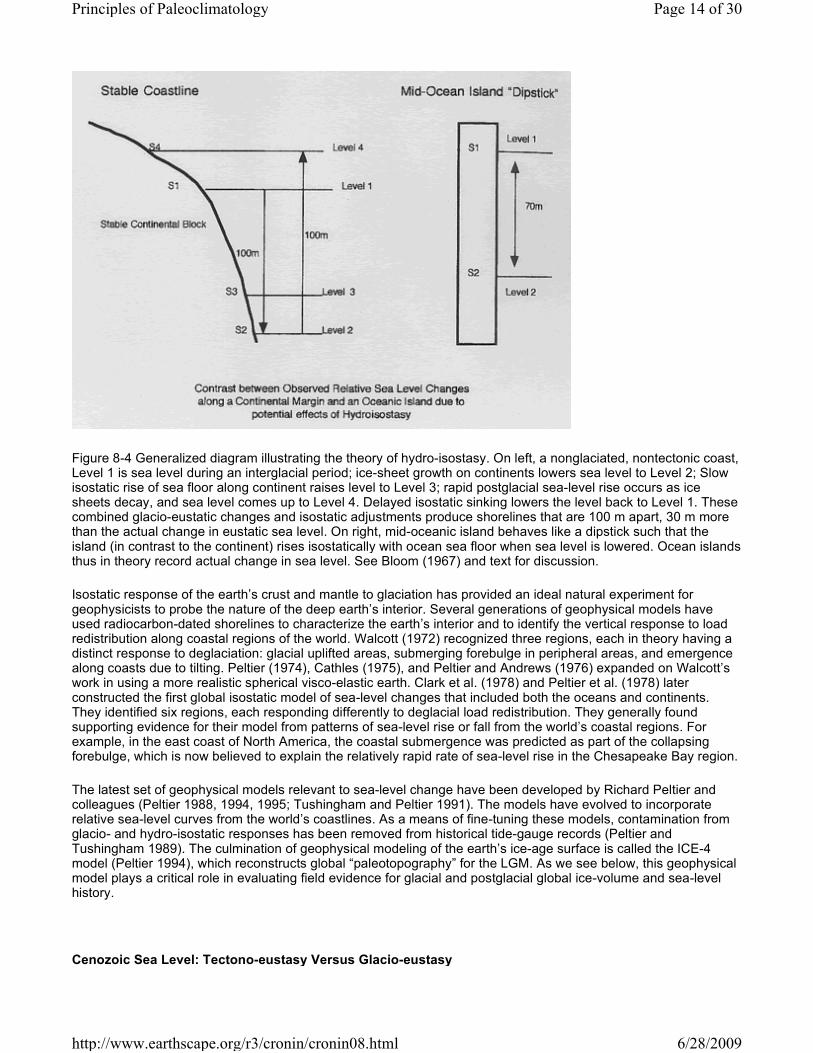
Figure 8-4 Generalized diagram illustrating the theory of hydro-isostasy. On left, a nonglaciated, nontectonic coast, Level 1 is sea level during an interglacial period; ice-sheet growth on continents lowers sea level to Level 2; Slow isostatic rise of sea floor along continent raises level to Level 3; rapid postglacial sea-level rise occurs as ice sheets decay, and sea level comes up to Level 4. Delayed isostatic sinking lowers the level back to Level 1. These combined glacio-eustatic changes and isostatic adjustments produce shorelines that are 100 m apart, 30 m more than the actual change in eustatic sea level. On right, mid-oceanic island behaves like a dipstick such that the island (in contrast to the continent) rises isostatically with ocean sea floor when sea level is lowered. Ocean islands thus in theory record actual change in sea level. See Bloom (1967) and text for discussion.

Isostatic response of the earth’s crust and mantle to glaciation has provided an ideal natural experiment for geophysicists to probe the nature of the deep earth’s interior. Several generations of geophysical models have used radiocarbon-dated shorelines to characterize the earth’s interior and to identify the vertical response to load redistribution along coastal regions of the world. Walcott (1972) recognized three regions, each in theory having a distinct response to deglaciation: glacial uplifted areas, submerging forebulge in peripheral areas, and emergence along coasts due to tilting. Peltier (1974), Cathles (1975), and Peltier and Andrews (1976) expanded on Walcott’s work in using a more realistic spherical visco-elastic earth. Clark et al. (1978) and Peltier et al. (1978) later constructed the first global isostatic model of sea-level changes that included both the oceans and continents. They identified six regions, each responding differently to deglacial load redistribution. They generally found supporting evidence for their model from patterns of sea-level rise or fall from the world’s coastal regions. For example, in the east coast of North America, the coastal submergence was predicted as part of the collapsing forebulge, which is now believed to explain the relatively rapid rate of sea-level rise in the Chesapeake Bay region.

The latest set of geophysical models relevant to sea-level change have been developed by Richard Peltier and colleagues (Peltier 1988, 1994, 1995; Tushingham and Peltier 1991). The models have evolved to incorporate relative sea-level curves from the world’s coastlines. As a means of fine-tuning these models, contamination from glacio- and hydro-isostatic responses has been removed from historical tide-gauge records (Peltier and Tushingham 1989). The culmination of geophysical modeling of the earth’s ice-age surface is called the ICE-4 model (Peltier 1994), which reconstructs global “paleotopography” for the LGM. As we see below, this geophysical model plays a critical role in evaluating field evidence for glacial and postglacial global ice-volume and sea-level history.

Cenozoic Sea Level: Tectono-eustasy Versus Glacio-eustasy



In 1977 Peter Vail and colleagues (Vail et al. 1977) of Exxon published a monograph on global eustatic sea-level changes used to interpret and correlate stratigraphic sequences of sedimentary basins around the world. Basing their sea-level curve on extensive seismic and biostratigraphic information accumulated during years of petroleum exploration, Vail and colleagues postulated that regional marine transgressions and regressions from passive continental margins could be used to erect a global sea-level curve (see also Vail and Hardenbol 1979). The sea-level curve was later referred to as a curve of onlap and offlap sequences in recognition of the fact that these sequences represented relative sea-level curves. The Vail curve stimulated a new generation of research into the long-dormant field of long-term eustatic sea-level history.

In brief, the Vail model of eustasy, resting on foundations built by L. Sloss, among others, held that periodic stratigraphic unconformities signified periods of regression and erosion and a hiatus in the deposition of marine sediments. Vail then applied this concept that seismic stratigraphy was a means to recognize sequences to develop a distinct set of criteria to identify strata within a sequence. Each complete sea-level cycle formed a distinct depositional sedimentary sequence–a comformable succession of genetically related strata bounded by unconformities. By convention, the sequence began with a sea-level low stand. Next, relative sea level rose again, forming a sedimentary sequence. During the third phase of a cycle, sea level dropped until it reached a low stand, which is reflected in the boundary unconformity. Vail classified sea-level cycles by the length of their period. For example, first-order cycles range over periods of hundreds of millions of years; third- and higher-order cycles occur over periods with frequencies of less than 5 Ma years. A revised eustatic sea-level curve covering the Mesozoic and Cenozoic was generated by Haq et al. (1987, 1988) and is now known as the Haq sea-level curve. Haq and colleagues also subscribed to the belief that global sea-level events could be recognized using sedimentary packages and dated and correlated using magnetostratigraphic and biostratigraphic data available for most sedimentary basins along continental margins.

In the same year that Vail et al. published their landmark paper, Anthony Hallam (1977) also published an important paper describing stratigraphic and paleontological evidence for long-term Phanerozoic patterns of marine inundation as a record of large-scale sea-level changes.

Since these influential papers, the Vail and Haq sea-level curves, in particular the chronology of post-Triassic coastal submergence and emergence and the mechanisms controlling long-term sea-level changes, have been actively researched and widely debated. Two major criticisms permeate the controversy. The first issue is geologists’ ability to date the events accurately enough to correlate among widely separated sedimentary basins and thus demonstrate the synchroneity of sea-level events. This problem applies especially to the correlation of third-order cycles, which in some sedimentary basins may represent regional changes in sediment supply or other processes unrelated to eustatic sea level (Christie-Blick et al. 1988). Miall (1997) was strident in criticizing the Vail-Haq sea-level curves because of limitations inherent in global correlation of sedimentary sequences and sea-level records. Miall demonstrated that random processes could produce the same sea-level patterns as those obtained from seismic records.

The second issue in the Vail and Haq sea-level curve controversy involves finding a mechanism that could explain the relatively rapid third- and higher-order events. Matthews (1988), for example, raised the issue as to whether the third- and fourth-order sea-level cycles were the result of glacio-eustasy. Morner (1981), in contrast, emphasized his long-standing opinion that geoidal and other effects render efforts to find a “global” sea-level curve futile. He stated that a global sea-level curve is “an illusion” because of geoidal effects–and he recommended that only regional eustatic curves be developed (p. 344). Haq and colleagues have defended both the age models used to correlate sea-level changes globally and the ability to correlate third-order cycles, vis-à-vis the number of sequences and the characteristic stacking.

Cenozoic deep-sea oxygen isotope records, ocean drilling on continental margins, and attempts to determine Antarctic ice-sheet history have recently shed new light on reconstructions of long-term sea-level history. The most important outcome of this research is that the Cenozoic Era was characterized by glacio-eustatic sea-level changes resulting from both North and South Polar regions. Antarctic ice-sheet oscillations have occurred since at least the earliest Oligocene (Barron et al. 1991), and Northern Hemisphere ice volume has fluctuated since at least the late Miocene, 7–10 Ma (Jansen et al. 1990; Jansen and Sjøholm 1991; Larsen et al. 1994). What follows is a brief summary of these findings.

Deep-Sea Isotope Records

Deep-sea oxygen isotope records of foraminifera were discussed in chapters 3 and 4 in terms of their value as a



monitor of continental ice volume. Early views that the steadily heavier oxygen values of the Cenozoic represented colder oceanic temperatures have been modified (Matthews and Poore 1980; Prentice and Matthews 1988) to suggest there is an ice-volume component to some foraminiferal isotopic records. Building on Quaternary deep-sea isotope research (Shackleton 1967; Shackleton and Opdyke 1973), Prentice and Matthews (1991) argued instead that the Cenozoic oscillations in deep-sea tropical planktic foraminiferal oxygen isotope values reflected a polar ice-volume history as far back as 40 Ma. Prentice and Matthews (1988) also developed the Snow Gun hypothesis to identify a mechanism whereby Antarctic ice growth might occur during periods of relative warmth, like the Miocene and Pliocene, driven by warming of deep water by low-latitude marginal seas. The Snow Gun theory held that, in contrast to ice-sheet growth related to cold deep-water formation of Quaternary glacial periods, warmer pre-Quaternary deep-sea waters may have contributed to Antarctic ice-sheet development.

Continental Margin Record

Sea-level history derived from stratigraphic and oxygen isotopic records from emerged and submerged sedimentary records from continental margins also indicate high-amplitude Cenozoic sea-level fluctuations. Miller et al. (1991) and Wright and Miller (1992) studied Oligocene and Miocene sea level along the eastern United

States and found 12 d18O spikes of > 0.5% in Oligocene and Miocene foraminifera. They interpreted the isotopic excursions as a sign that sea level fell between 20 and 80 m during low stands. Pekar and Miller (1996) found 10 major unconformities in records from Ocean Drilling Program (ODP) legs off New Jersey that matched periods of low sea level in the Haq curve. The amplitude of Oligocene sea-level changes were, however, only 24–34 m, about one half the amount postulated by Haq and colleagues. McGinnis et al. (1993) offered a mechanism to explain the smaller magnitude of Tertiary sea-level events obtained from continental margin ODP legs and the Haq curve. They suggest that the early-late Oligocene (38–34 Ma) sea-level fall, estimated by Haq to be as much as 150 m, is overestimated because part of the observed relative sea-level fall is the result of flexural isostatic rebound of the lithosphere along the continental margin due to deep-sea erosion and retreat of the continental slope.

Miller et al. (1996) integrated evidence from sequence stratigraphy from ODP cores and onshore coastal plain deposits in New Jersey with oxygen isotope curves to draw an improved sea-level curve for the Oligocene–middle Miocene that generally supported the Haq model for global Cenozoic third-order sea-level oscillations. They found

an excellent correspondence among seismic reflectors, increases in d18O of foraminifera (indicating reduced ice volume), and coastal plain unconformities, all indicators of lowered sea level. Miller and colleagues argued that between 36 and 10 Ma, multiple sea-level cycles occurred over million-year time scales. About 10 cycles punctuated the period 12–24 Ma, one occurring about every 1–2 Ma. Data from ODP Leg 166 of the Bahama Banks lent similar support for eustatic Cenozoic sea-level change.

The Glacial Record

Are the alleged glacio-eustatic sea-level oscillations hypothesized from isotopic and continental margin stratigraphic records supported by direct evidence for ice-volume instability from polar regions (Mangerud et al. 1996)? Quite likely. It is now generally accepted that continental-scale ice existed in Antarctica since the earliest Oligocene, about 40 Ma (Barron et al. 1991; Ehrmann et al. 1992) and in Greenland since at least 7 Ma (Larsen et al. 1994). Extensive stratigraphic, ice-rafting, and micropaleontological evidence has been obtained from ODP legs such as Leg 119 from the Kerguelen Plateau region and other sites near Antarctica (Barron et al. 1991). However, even as Antarctic and Greenland ice-sheet history begins to emerge from glaciological, isotopic, stratigraphic, lithological, and ice-rafted debris (IRD) evidence in deep-sea sediments, sea-level history due to polar ice-volume instability remains elusive. To illustrate this complexity, I examine the debate surrounding late Neogene Antarctic Ice Sheet stability.

The debate revolves around how dynamic the Antarctic ice sheet has been for the past 6 Ma or so. The stabilist view (Sugden et al. 1993; Kennett and Hodell 1993) holds that Antarctic ice volume has remained fairly stable since at least the Miocene. This conclusion is based mainly on geomorphological, glaciological, and chronological evidence from several regions of Antarctica (Denton et al. 1993), glacial modeling (Huybrechts 1993), deep-sea ice rafting data, and stable-isotope data. Kennett and Hodell (1993) reviewed evidence for ice rafting around Antarctica, a line of evidence signifying the existence of a large ice sheet. They concluded (p. 213) that “the Subantarctic IRD records an expansion of the Antarctic cryosphere during the latest Miocene through earliest Pliocene, relative stability during the early Pliocene, and further expansion during the late Pliocene.”

The dynamicist view is based on stratigraphic and paleontological evidence from several regions of Antarctica, suggesting one third to one half deglaciation during parts of the Pliocene over the past 5 Ma (Webb et al. 1984;



Webb and Harwood 1991; Wilson 1995). Independent evidence for relatively high sea level during the Pliocene (Haq et al. 1987; Dowsett and Cronin 1990; Wardlaw and Quinn 1991) suggests there may have been partial deglaciation of Antarctica.

The long-term history of the Greenland Ice Sheet has emerged within the past few years from deep-sea sedimentology and isotopic records. Greenland ice began building up in the late Miocene, perhaps as much as 8–10 Ma. Jansen et al. (1990) found ice-rafted sediments, diamictons, and dropstones as old as 6 Ma in ODP sediments from the Norwegian Greenland Sea. Jansen and Sjøholm (1991) estimated glacio-eustatic sea level drops near 5.0 and 3.9 Ma to have been as much as 60–100 m based on combined IRD and oxygen-isotope data from the Norwegian Sea. After about 2.75 Ma, there was intensification of Northern Hemisphere glaciation with European glaciation beginning around 2.57 Ma (Jansen and Sjøholm 1991).

Additional evidence for dynamic Northern Hemisphere ice comes from Greenland, where Larsen et al. (1994) discovered glacial till, diamictons, and dropstones in deep-sea cores from off the southern coast of Greenland. They concluded that cooling around Greenland started after 10 Ma and full glacial conditions developed by 7 Ma. These events may have led to a glacio-eustatic sea-level drop of 12 m. These and other studies indicate a significantly more complex and dynamic late Miocene and Pliocene glacial history of the Northern Hemisphere than researchers recognized just a decade ago and provide a mechanism for pre-Quaternary low-amplitude glacio-eustatic sea-level changes (Mangerud et al. 1996). Evidence for sea ice in the Arctic Ocean extends back at least until 12–14 Ma (Thiede et al. 1996), but sea-ice would not have affected eustatic sea level.

In closing this brief discussion on long-term sea-level history, it should be emphasized that some geologists remain skeptical that long-term Phanerozoic eustatic cycles are glacio-eustatic in nature (Dott 1992). Similarly, there is perhaps even more skepticism surrounding the idea that pre-Cenozoic sea-level cycles reflect orbital-scale sea-level changes (Sloss 1991; see chapter 4). Moreover, disputes about the long-term contribution of Antarctic and Greenland ice to eustatic sea level will likely continue into the foreseeable future. Regardless of the outcome of these debates, there is growing evidence that since their initial formation > 35 Ma and > 7 Ma, respectively, Antarctic and Northern Hemisphere polar ice sheets have undergone dynamic oscillations that were probably large enough in many instances to cause sea-level oscillations of at least 10–30 m over time scales of 100 ka to 1 Ma. The possibility that Cretaceous sea-level fluctuations are glacio-eustatic in origin remains a viable hypothesis as well (Stoll and Schrag 1996). Still, it remains a major challenge to decouple glacio-eustatic sea-level changes related to climate change from those produced by other mechanisms and to reconstruct long-term sea-level changes.

Quaternary Sea-Level History

In chapter 4, I described the contribution that Quaternary sea-level history has made to testing the basic tenets of the orbital theory of climate change. The age and elevation of tectonically uplifted coral reef terraces in Barbados and New Guinea record swings in sea level over tens to hundreds of thousands of years that according to many researchers match the timing of ice-volume fluctuations inferred from deep-sea oxygen isotope curves and times of low solar insolation. During the past 500 ka, each 100-ka glacial-interglacial cycle underwent a low sea level, about 100 m below the present level, and a high sea level within a few meters of the current level. The dominant 100-ka period corresponding to the period of orbital eccentricity was superimposed on sea-level high stands occurring about every 20 ka, associated with earth’s precessional period. During most of the past 500 ka, sea level has remained below its current level because the volume of ice stored on continents was greater than it is now. During the late Pliocene and early Pleistocene (2.5–0.5 Ma), eustatic sea level oscillated at the 41-ka orbital frequency but at a lower amplitude, perhaps 40–60 m (Raymo et al. 1989; Ruddiman et al. 1989; Cronin et al. 1994; Naish 1997). Together, the paleoclimatological record from emerged coral terraces, coastal stratigraphy, and deep-sea isotopes have led to a widespread, though not universal, acceptance of the influence of orbital factors on late Cenozoic global climate, the cyclic waxing and waning of glaciers, and glacio-eustatic oscillations.

In addition to Cenozoic orbital-scale cyclic ice-volume and sea-level changes, reconstructing sea level during the LGM and the progressive sea-level rise and ice-sheet decay during deglaciation are two of the most important topics in paleoclimatology. The next two sections discuss sea-level controversies surrounding sea level and global ice volume during the LGM and the subsequent deglaciation. The evidence for relative sea-level changes over the past 20 ka is scattered throughout the literature, in part because regional field studies have been carried out on so many of the world’s coastlines. Recognizing the importance of correlating relative sea-level curves, the



International Geological Correlation Program (IGCP) has sponsored four successive international projects over the past 20 years to examine late Quaternary relative sea-level history and to sort out eustatic, geoidal, and isostatic effects. These projects have been coordinated by leading sea-level researchers–Arthur Bloom, Paolo Pirazzoli, Orson van de Plassche, and David B. Scott–and have resulted in many field excursions and publications on regional sea-level history (e.g., Bloom 1992).

In addition to extensive field studies, late Quaternary sea-level research depends heavily on accurate chronology of sea-level events. Excellent summaries of Late Quaternary relative sea-level obtained from continental margins

using conventional 14C can be found in Bloom (1977) and Pirazzoli (1991). In addition, recent improvements in the

chronology of sea-level history have come from accelerator mass spectrometric (AMS) 14C and uranium-series thermal ionization mass spectrometry (TIMS) dating (Bard et al. 1990a,b, 1992, 1993).

Thick Ice and Thin Ice During the Last Glacial Maximum

The thickness of late Quaternary ice sheets has been debated for at least a century and a half. During the formative days of Agassiz’s glacial theory, Maclaren (1842) had already estimated that sea level would be lower by 350 feet because of ice locked up on the continents, even excluding ice in the south polar region. Later, Penck (1882) also estimated a glacio-eustatic sea-level drop of 100 m. These were remarkably accurate estimates foreshadowing most currently accepted estimates, which range from 100 to 130 m.

Currently, the problem of how far sea level fell during the LGM about 21 ka remains intimately related to conflicting estimates of continental ice volume and past sea-level positions at the continental shelf edge. Two opposing viewpoints can be expressed in terms of the thickness of the last great ice sheets (in order of decreasing volume): the Antarctic, Laurentide of eastern Canada and the midwestern and northeastern United States (figure 8-5), Fennoscandinavian, Barents-Kara Sea in the eastern Arctic Ocean, Greenland, Cordilleran in the Pacific northwest extending into southern Alaska, Innuitian in the Canadian Arctic island archipelago, northern British Isles, and Icelandic. It should be noted that the extent of the Barents-Kara Sea ice sheet has been a topic of some debate (e.g., Denton and Hughes 1981; Grosswald 1993, see below) and that there were other smaller ice caps, especially at high elevations, I have not listed.

Historically, one school of thought has adhered to a “thick ice scenario” in which, at their greatest extent, LGM ice sheets held the equivalent of as much as 130–160 m of sea level. The other theory holds to a “thin ice scenario,” which calls for thinner ice sheets and a much smaller fall in eustatic sea level of about 100 m (table 8-2).

The evidence upon which each ice-volume–sea-level scenario rests, however, comes from a spectrum of complex topics that include coral reef accretion and growth, ice mechanics, earth rheology, stable-isotope fractionation, foraminiferal ecology, salt marsh accretion, and others.



Figure 8-5 Late Quaternary North American Laurentide Ice from about 14 ka, about the time of meltwater pulse 1a. Courtesy of Peter Clark and the American Geophysical Union. From Clark et al. (1996a).

Table 8-2. Selected Estimates of Global Sea Level During the Last Glacial Maximum

*CLIMAP Project members (1981) used these studies for their LGM estimates.

§Includes for tectonic uplift about 0.34 mm/yr, or 7 m since the LGM.

Sea level and ice volume during the LGM and the succeeding deglaciation has been reconstructed through four main avenues of investigation. First is the combination of glacial geology, carried out by extensive field mapping of glaciated and periglacial regions in middle and high latitudes (e.g., Andrews et al. 1993b, 1995b, references therein; Denton and Hughes 1981; Dyke and Prest 1987; Sibrava et al. 1986), and glaciological modeling (Denton and Hughes 1981; Clark et al. 1996b) that addresses glacial mechanics and the way ice sheets respond to various

Estimate Study Sea-level change (m)

CLIMAP maximum Denton and Hughes 1981 163*

CLIMAP minimum Denton and Hughes 1981 127*

Barbados Fairbanks 1989 125§

ICE-4 Peltier 1994 105



boundary conditions and forcing. The global LGM ice reconstruction of Denton and Hughes (1981) was used in the CLIMAP project, and it provided two extreme ice reconstructions. The maximum ice sheet reconstruction called for

97.8 x 106 km2 total volume of ice, of which 65.3 x 106 km2 would lower sea level; the rest was floating marine ice

sheets. The minimum LGM reconstruction is estimated at 84.2 x 106 km2 total ice volume, of which 51.3 x 106 km2 contributed to a sea-level drop. These maximum and minimum ice configurations were the equivalent to 163 and 127 m of sea-level drop, respectively, which after taking into account isostatic effects would produce eustatic sea-level drops of 117 and 91 m. The Denton and Hughes Laurentide Ice Sheet reconstruction held that there was a single dome located over Hudson Bay where surface elevations exceeded 3800 m. This thick ice scenario was used by CLIMAP (1981) and other researchers modeling glacial-age climate.

The CLIMAP ice sheet reconstructions and sea-level estimates for the LGM, however, were not always accepted (see Andrews et al. 1986) and have since been modified. One important factor requiring reevaluation of ice sheet thickness is the nature of the subglacial bed throughout glaciated regions. Clark et al. (1996b) recently revised long-standing concepts about the thickness of the Laurentide Ice Sheet in North America that characterize the CLIMAP reconstructions by applying a different viewpoint on subglacial sediments. Specifically, they noted that geological field evidence indicates that large parts of the land surface below the Laurentide Ice Sheet consisted of relatively wet, easily deformable glacial till, referred to as “soft bed” till by Clark et al. (1996b). In contrast to areas where the subglacial substrate is more rigid and ice flow is influenced mainly by ice deformation, the wet, soft till substrate influences ice flow both by ice deformation and by sediment (i.e., till) deformation. By applying this twofold classification of hard bed and soft bed substrate to crystalline and sedimentary bedrock regions, respectively, to a numerical reconstruction of the Laurentide Ice Sheet, Clark et al. (1996b) found evidence for a much thinner Laurentide Ice Sheet than previous studies had indicated. Their paleo-topography showed four ice domes instead of one, one on either side of James Bay, one in the Keewatin district west of Hudson Bay, and one over the Foxe Basin. They depict the overall features of the ice sheet as follows (p. 681):

In general, the ice-sheet surface topography is best described as a broad plateau with elevations 2000–2500 m asl [above sea level] centered over the area of crystalline bedrock and surrounded on its southern, western, and northwestern sides (corresponding to areas of low-viscosity till) by a low brim of ice ranging in elevation from 500–1500 m asl.

This thin ice sheet scenario calls for a Laurentide Ice Sheet volume that is 75% thinner than the estimated maximum volume of Denton and Hughes (1981). Obviously it would result in a much smaller sea-level drop during the LGM. Whereas these ice sheet reconstructions involve numerous assumptions and potential sources of uncertainty, other methods of ice volume reconstruction discussed next tend to support the thin ice model.

The second approach to reconstructing glacial sea level is to determine past sea-level positions directly from ancient shorelines using stratigraphic, geomorphological, and paleobiological study of submerged shorelines and coastal environments preserved at various elevations below modern sea level (e.g., Bloom et al. 1974; Pirazolli et al. 1989; Tooley and Shennan 1987). During the 1960s and 1970s, radiocarbon dating of shells, peats, and other material from outer continental shelves produced the earliest sea-level curves (Fairbridge 1961; see Pirazolli 1991), but relatively few dates were found that were old enough to define sea level during the LGM (Field et al.

1979). For example, in the Newman et al. (1980) compilation of 4000 14C dates, only about 40 are older than 14 14C ka, and of these, only a dozen or so are from water depths > 80 m below sea level. The remainder of the dates come from subsequent periods of deglaciation, when sea level had already risen from its glacial low stand. Such is also the case for Pirazzoli’s (1991) compilation of 900 sea-level curves from the world’s coastal regions.

In addition to problems of tectonic and isostatic subsidence and uplift in many regions, several other problems prevented early workers from establishing an accurate sea-level position for the LGM from continental margin shoreline sediments. One of the problems was that some types of dated organic material, such as fossil mollusk shells, did not come from the original water depth at which they lived (that is, postmortem sedimentary processes had transported them into deeper water). Another dilemma was whether the dated species (e.g., the oyster Crassostrea virginica) had lived precisely at sea level or many meters below mean sea level and thus provided only a minimum depth for a paleo–sea-level position.

This situation changed radically when submerged coral reefs from the Caribbean Island of Barbados, radiocarbon dated by Fairbanks (1989), and Muruao Atoll in French Polynesia, dated by the uranium-series TIMS method by Bard et al. (1992, 1993), provided a much better source of direct paleo-shoreline data from the LGM. Corals provided a stable sea-level datum from which to evaluate LGM sea level. Fairbanks (1989) obtained a transect of cores from 50–130 m depth off Barbados that penetrated fossil reefs of the coral Acropora palmata, the same



species of coral used successfully to document high sea-level events from emergent reefs associated with orbital climate change (see chapter 4). A. palmata is a well known species of coral ideally suited to paleo–sea-level studies because its ecology limits its depth range to < 5 m in most regions (Lighty et al. 1982). The deepest submerged fossil A. palmata, lying at 113 m below sea level, was dated by radiocarbon at 17.1 ka and later by uranium series dating (Bard et al. 1992). This remains the single best-dated LGM sea-level datum available. Assuming tectonic uplift was about 7 m since the LGM, and given the < 5-m depth range of A. palmata, Fairbanks (1989) estimated glacial eustatic sea level was about –121 ± 5 m. A sea-level fall of 121 m lies toward the lower end of estimates derived from glaciological evidence used in the CLIMAP studies.

A third method used to estimate LGM sea level is geophysical modeling that investigates the earth’s short-term vertical isostatic response to redistribution of load due to continental ice growth and decay (Clark et al. 1978; Tushingham and Peltier 1991; Peltier 1994). Peltier’s geophysical model to describe “ice age paleotopography” is called the ICE-4 model. ICE-4 calculates paleotopography for the earth during the LGM using a visco-elastic model of the earth’s response to ice-sheet melting. The model essentially uses hundreds of relative sea-level curves from around the world to constrain earth’s crustal and mantle isostatic adjustment to deglaciation and create an inverse curve. It is constructed from the earlier ICE-3 model (Tushingham and Peltier 1991), which was tuned to sea-level curves mostly from glaciated areas and mostly covering the past 8 ka. The ICE-4 model described by Peltier (1994, 1995) is significantly improved in that it is tuned to the uncorrected Barbados LGM sea-level depth of 118 m (Fairbanks 1989).

The ICE-4 model estimates eustatic sea level at 21 ka to be about 105 m below present. The 105-m eustatic sea-level estimate is 13 m below the uncorrected depth of the 21 ka radiocarbon dated Barbados A. palmata coral because of geoidal and isostatic effects (Peltier 1995). Although the ICE-4 model has been criticized for underestimating eustatic sea level because it does not take into account presumed uplift of Barbados during the past 21 ka (Edwards 1995), Peltier responded that isostatic disequilibrium could easily account for the difference. Moreover, even if the uplift of 7 m were incorporated into the ICE-4 model, the estimated ice-sheet thickness would change by only 200 m, an inconsequential amount in terms of the use of ice-age paleotopography in studies of atmospheric general circulation modeling of glacial climates. The critical conclusion derived from the ICE-4 model is that LGM ice sheets were significantly thinner–about 35% thinner than many prior estimates and as much as 1000 m thinner for portions of the Laurentide Ice Sheet–than the CLIMAP LGM ice-sheet reconstructions.

Figure 8-6 Comparison of New Guinea sea-level curve and the ice-volume curve obtained from deep-sea Pacific Ocean benthic foraminiferal oxygen isotopes for the past 130 ka. The discrepancy between the two records most



likely results from the contribution of deep-sea temperature changes to the oxygen isotopic signal. Courtesy of A. Mix, with permission from the Geological Society of America. From Mix (1992).

A fourth, less direct method of estimating glacial sea level comes from the deep-sea foraminiferal oxygen-isotope record of ice-volume history (figure 8-6). As discussed in chapter 2 and elsewhere in this book, oceanic oxygen isotopic composition reflects in part continental ice-sheet volume because of differential fractionation of the light

and heavy oxygen isotopes, so that the 18O:16O ratios of deep-sea foraminifers record changes in ice volume (Shackleton and Opdyke 1973; Chappell and Shackleton 1986; Schrag et al. 1996). The oxygen isotopic method of estimating ice volume has the advantage of being unaffected by isostatic and tectonic effects. Using the calibration of 0.11% per 10 m of sea level (Fairbanks and Matthews 1978), and all other factors being equal, a typical 1.5–1.7% oxygen isotopic shift between glacial age and modern foraminifers would imply a fall in sea-level change during the LGM of as much as 150–170 m. However, the isotope signal in foraminifers is also affected by other factors, the most important being ocean temperature changes. Given the evidence discussed earlier that tropical sea-surface temperatures (SSTs) dropped during the LGM and that deep-sea bottom water temperature fell at

least 1.5–2.0oC globally (Labeyrie et al. 1987; Chappell and Shackleton 1986) and as much as 2.5–3.0oC in the

Atlantic Ocean (Dwyer et al. 1995), estimating eustatic sea-level change from foraminiferal d18O requires care. In general, reevaluation of the ice volume signal from oxygen isotopes that takes glacial-age reductions in surface and deep bottom water into account would place the isotopic LGM ice volume estimates more in line with those derived from new glacial geological interpretations, the Barbados coral record, and geophysical modeling.

In sum, while the above discussion is a great oversimplification of the complex topic of LGM ice reconstruction, it serves to characterize the two opposing points of view and the types of paleoclimate evidence garnered to support each. Recent evidence from glaciological data, coral paleo–sea level, geophysical modeling, and revised oxygen-isotope results suggests that glacial-age ice sheets may have been substantially thinner than was thought 15–20 years ago. This concept has serious implications for the rate of sea-level rise during subsequent deglaciation.

Late Quaternary Deglaciation and Sea-Level Rise

The period between 21 and 6 ka, when late Quaternary ice sheets melted, can be divided into four stages based on the Barbados sea-level curve of Fairbanks (1989) and other sea-level records referenced later (figure 8-7). The first, early deglaciation about 21.0–14.5 ka, was a time when the Barents Ice Sheet may have disintegrated. The second, about 14.5–12.5 ka, is called Meltwater Pulse (MWP) 1a and includes a rapid pulse of melting about 14.2–13.8 ka. Most researchers believe a large portion of the Laurentide Ice Sheet collapsed during MWP 1a, although recently Clark et al. (1996a) suggested that maybe parts of Antarctica may have played a role. The third period corresponds to the Younger Dryas, 12.5–11.5 ka, when the rate of sea-level rise slowed appreciably. The fourth stage was Meltwater Pulse 1b, centered about 11.6–11.1 ka, when the Fennoscandianvian Ice Sheet and probably a portion of the Antarctic Ice Sheet melted.



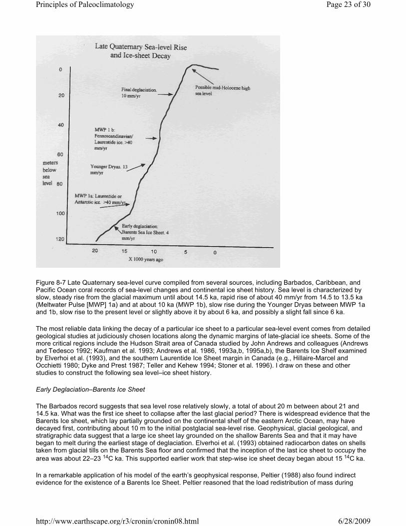
Figure 8-7 Late Quaternary sea-level curve compiled from several sources, including Barbados, Caribbean, and Pacific Ocean coral records of sea-level changes and continental ice sheet history. Sea level is characterized by slow, steady rise from the glacial maximum until about 14.5 ka, rapid rise of about 40 mm/yr from 14.5 to 13.5 ka (Meltwater Pulse [MWP] 1a) and at about 10 ka (MWP 1b), slow rise during the Younger Dryas between MWP 1a and 1b, slow rise to the present level or slightly above it by about 6 ka, and possibly a slight fall since 6 ka.

The most reliable data linking the decay of a particular ice sheet to a particular sea-level event comes from detailed geological studies at judiciously chosen locations along the dynamic margins of late-glacial ice sheets. Some of the more critical regions include the Hudson Strait area of Canada studied by John Andrews and colleagues (Andrews and Tedesco 1992; Kaufman et al. 1993; Andrews et al. 1986, 1993a,b, 1995a,b), the Barents Ice Shelf examined by Elverhoi et al. (1993), and the southern Laurentide Ice Sheet margin in Canada (e.g., Hillaire-Marcel and Occhietti 1980; Dyke and Prest 1987; Teller and Kehew 1994; Stoner et al. 1996). I draw on these and other studies to construct the following sea level–ice sheet history.

Early Deglaciation–Barents Ice Sheet

The Barbados record suggests that sea level rose relatively slowly, a total of about 20 m between about 21 and 14.5 ka. What was the first ice sheet to collapse after the last glacial period? There is widespread evidence that the Barents Ice sheet, which lay partially grounded on the continental shelf of the eastern Arctic Ocean, may have decayed first, contributing about 10 m to the initial postglacial sea-level rise. Geophysical, glacial geological, and stratigraphic data suggest that a large ice sheet lay grounded on the shallow Barents Sea and that it may have began to melt during the earliest stage of deglaciation. Elverhoi et al. (1993) obtained radiocarbon dates on shells taken from glacial tills on the Barents Sea floor and confirmed that the inception of the last ice sheet to occupy the

area was about 22–23 14C ka. This supported earlier work that step-wise ice sheet decay began about 15 14C ka.

In a remarkable application of his model of the earth’s geophysical response, Peltier (1988) also found indirect evidence for the existence of a Barents Ice Sheet. Peltier reasoned that the load redistribution of mass during



deglaciation would alter two components of earth’s planetary rotation: the nontidal component of acceleration of the earth’s axial rate of rotation and the drift of the rotation pole with respect to surface geography. Basically, the earth’s rotation speeds up as the ice sheets melt and load is transferred to the oceans. Peltier used modern satellite geodetic data to infer that both rotational components did not fit with the accepted current rate of sea-level rise of about 0.5 mm/yr (e.g., Meier 1984). To account for the discrepancy, an additional mass of ice, unknown to exist on the continents, was necessary. Peltier suggested that during the last glacial period a large ice mass in the general vicinity of the Barents Sea would account for the modeling results.

Jones and Keigwin (1988) provided support for the existence of a Barents Sea Ice Sheet in a study of oxygen-isotope records from the Fram Straight, the only deep-water oceanic gateway to the Arctic Ocean, situated between Spitzbergen and northern Greenland. They found an isotopic excursion dated by AMS radiocarbon dates that preceded the characteristic deglacial two-step isotopic spike of Termination 1 by 1–2 ka. They hypothesized that this represented a significant meltwater event, when fresh water discharge from the Barents Ice Sheet caused lighter isotopic ratios in the planktonic foraminifer, Neoglobigerina pachyderma. Because this isotopic spike was not accompanied by a large rise in sea level, however, they suggested that it might be due to ice sheet decay from an ice mass grounded wholly or partially below sea level.

Additional evidence for a large ice sheet in the eastern Arctic Ocean came from the Yermak Plateau, where Vogt et al. (1994) discovered iceberg plowmarks along the ocean bottom in 450–850 m water depth. They interpreted these as recording a 400- to 600-m-thick Arctic Ocean ice sheet calving from a Barents and Kara Sea source area. The estimated weight of these “megabergs,” as Vogt et al. refer to them, was 107–108 tons. Iceberg keel marks formed on the ocean floor during the past ice age were also found off Norway, Greenland, and Baffin Island, Canada. Although the iceberg keels are not well dated, Polyak et al. (1995) documented independent stratigraphic and micropaleontological evidence in the Barents Sea itself for early deglacial ice sheet disintegration that was followed by a larger two-step deglaciation. Taken together, these studies suggest a dynamic breakup of a marine-based ice sheet.

A final line of evidence for early Barents Ice Sheet decay comes from the ingenious use of lithologic provenance by Bischoff (1994), who determined the sequence of late glacial oceanic sedimentation on the Vøring Plateau off the west coast of Norway. During the glacial maximum, most glacially derived sediment in the eastern Norwegian Sea originated in the Fennoscandinavian ice sheet to the east. As deglaciation began, there was a dramatic change in

ice-rafted drop-stone lithology in the marine sediments dated at 15.0–14.5 14C ka. This age coincides with the isotopic shift of Jones and Keigwin (1988) and also with the stratigraphic and faunal changes of Polyak et al. (1995). Vøring Plateau sediment shifted from crystalline rocks to coarse sand and gravels nearly identical to those sediments that cover the Barents Sea shelf, implying a change to the Barents Sea as the drop-stone source area. Bischoff estimated that sedimentation rates increased 10-fold during initial deglaciation (in calendar years about 18–17 ka) and conjectured that this lithological transition was remarkably swift, occurring in just 400 yr. Following this catastrophic ice decay, there was a more gradual 4.5-ka-long disintegration of the remaining ice sector in the Spitzbergen-Svalbard area.

In summary, considerable evidence indicates that an ice shelf was present in the Barents Sea area and that much of it probably melted catastrophically relatively early in the postglacial period, perhaps followed by more gradual disintegration of the remainder.

Meltwater Pulse 1a

Fairbanks (1989) proposed that sea level rose 24 m in less than 1000 years during MWP 1a based on the radiocarbon-dated Barbados coral A. palmata–the first rapid postglacial rise in sea level signifying massive

continental ice-sheet decay. Meltwater Pulse 1a discharged about 14,000 km3/yr into the North Atlantic, an amount

equivalent to all North Atlantic river discharge between 0–90oN latitude. Blanchon and Shaw (1995) further analyzed the Barbados sea-level record and argued that one could distinguish three rates of sea-level rise in the Barbados stratigraphic record based solely on coral ecology and taphonomy. During relatively slow sea-level rise of < 14 mm/yr, the occurrence of monospecific A. palmata assemblages track sea-level rise because this species’ ecology allows it to accrete its skeleton at rates below this threshold. When sea level rises at rates > 14 but < 45 mm/yr, the Barbados stratigraphy shows that A. palmata corals are displaced into a mixed coral assemblage that is more characteristic of a water depth range of 5–10 m. At exceptionally rapid rates of sea-level rise, > 45 mm/yr, sea level rises too fast even for a mixed coral reef framework to develop.

Blanchon and Shaw applied this model of coral paleobiology and taphonomy to identify A. palmata reefs that were



drowned by rising sea level. They found three horizons at 80, 50, and 15 m below sea level in Fairbanks’s Barbados core where sea level rose at a rate exceeding 45 mm/yr. These were dated near 14.2–13.8 ka (MWP 1a), 11.5 ka (MWP 1b), and 7.6 ka. Each date signifies a catastrophic, that is, within a few centuries, sea-level rise equivalent to 13.5, 7.5, and 6.5 m, respectively. Where did the meltwater come from?

The origin of MWP 1a has long been held to represent meltwater from the Laurentide Ice Sheet. The evidence for this conclusion comes from glacial geology on the continent (Teller and Kehew 1994), oxygen-isotope evidence for meltwater events in the deep-sea record (Keigwin et al. 1991), and ice-rafted material in the North Atlantic (Bond et al. 1992). Drainage of freshwater outflow via the Mississippi River was believed responsible for isotopic excursions recorded in Gulf of Mexico foraminifers (Leventer et al. 1983) and the Bermuda Rise (Keigwin et al. 1991).

Clark et al. (1996a), however, recently argued against the Laurentide Ice Sheet as a source for MWP 1a for at least two reasons. First, the amount of ice available in the sector of the ice sheet draining via the Mississippi River outlet was insufficient to cause the observed isotopic excursion. Second, the rate of ice ablation was implausible given current knowledge about ice sheet sensitivity to temperature change. Clark’s group argues that evidence from glacial IRD and stable isotopes from the two other outlets of the Laurentide Ice Sheet, the Hudson Strait (Andrews et al. 1993a, 1994) and the St. Lawrence River (Hillaire-Marcel et al. 1993; de Vernal et al. 1996; Stoner et al. 1996), indicate no major IRD pulses were synchronous with MWP 1a and the corresponding period of rapid sea-level rise. Moreover, Heinrich events in the North Atlantic Ocean were not synchronous with MWP 1a, as might be expected if they were caused by Laurentide Ice Sheet decay (Bond et al. 1992, 1993). These data led Clark and colleagues to radically alter the concept of MWP 1a from that of a Laurentide Ice Sheet event to an Antarctic Ice Sheet event. They theorized that Antarctic ice had, in fact, contributed to most of the meltwater discharge about 14–13 ka. In doing so, they add a new dimension to the reconstruction of late Quaternary sea-level history with implications for thermohaline circulation and mechanisms of late Quaternary climate change as well.

Younger Dryas Sea Level

The Younger Dryas stadial is represented in the sea-level record at Barbados in the form of a much reduced rate of sea-level rise and a meltwater equivalent about one fifth the volume of MWP 1a (Fairbanks 1989). A sea-level curve based on radiocarbon-dated corals from a core from the Huon Peninsula, New Guinea (Chappell and Polach 1991), does not contradict the inferred slower Younger Dryas rate of sea-level rise. Fairbanks argued that the Younger Dryas was essentially a period of reduced meltwater discharge sandwiched between two periods of massive meltwater discharge and reduced oceanic surface salinities. Fairbanks suggested that this relationship is the opposite of that between meltwater discharge, surface salinity, and climate cooling in the North Atlantic region proposed by Broecker et al. (1988b) as an explanation for the Younger Dryas cold snap (see chapter 5). This distinction is critical for explanations of the Younger Dryas event, but all that is important here is to note that the rate of sea-level rise was substantially reduced from that just prior the Younger Dryas. Blanchon and Shaw (1995) estimated Younger Dryas A. palmata accretion and sea-level rise to be 13 mm/yr, much slower than the catastrophic 45 mm/yr rate during MWP 1a, but more rapid than the earliest deglaciation rate of 4 mm/yr 20–15 ka.

There is abundant glacial evidence for ice-sheet readvances and reduced rates of glacial retreat around the time of the Younger Dryas cold episode. For example, Polyak et al. (1995) found a period of nondeposition of glacio-marine sediments reflecting a pause in the decay of the remnants of the Barents Sea ice sheet near the Younger Dryas time. A detrital carbonate event signifying ice-stream discharge of Heinrich event–like icebergs is also evident in Hudson Strait (Andrews and Tedesco 1992; Andrews et al. 1993a,b, 1995a).

Meltwater Pulse 1b

Sea level rose a total of about 28 m during MWP 1b, centered at about 11.5–11.0 ka (Fairbanks 1989) at a rate exceeding 45 mm/yr (Blanchon and Shaw 1995). Chappell and Polach (1991) also recorded rapid sea-level rise during coral reef accretion in New Guinea. There are several possible ice sheet sources for MWP 1b. One is the northern region of Labrador where Kaufman et al. (1993) documented several major advances of Laurentide ice between 14 and 9 ka. The most rapid and well-dated advance is the abrupt Gold Coast advance of the Labrador dome of Laurentide ice. Kaufman and colleagues cite evidence that the ice advanced as much as 300 km along a 200-km-long calving ice sheet margin into the Hudson Strait area. The entire advance-retreat cycle was completed within only about 300 years. They estimated that this advance might account for as much as one fourth of the total sea-level rise during MWP 1b. The Gold Coast advance apparently did not significantly affect North Atlantic ocean salinities and circulation, either because it did not produce a sufficient quantity of icebergs or their ocean trajectories were too far to the south. The remainder of the MWP 1b sea-level rise most likely came from



Fennoscandinavia and/or eastern North America through the St. Lawrence River.

Three points about the evidence for this sequence of late Quaternary postglacial sea-level history need to be emphasized. First, widely divergent opinions remain about which ice sheet contributed to each stage of the postglacial sea-level rise; we have only briefly touched upon some of the more recent theories. The uncertainty in deglacial ice sheet–sea level chronology stems in part from a relatively poor chronology of Antarctic late glacial history compared with that from the Northern Hemisphere. The chronology is also uncertain because meltwater events from the deep sea isotope record are subject to various interpretations.

Second, the chronology of the postglacial sea-level record does not yet approach the near-calendar year chronology available from some European terrestrial and Greenland ice core records (chapters 5, 9). There are only a limited number of well-dated postglacial sea-level records from submerged shorelines for the interval spanning the glacial maximum through early deglaciation before about 10 ka. Even in the case of the Barbados curve, rates of sea-level rise must be interpolated between relatively few radiocarbon dates for the periods of most rapid deglaciation. The lack of calendar-year chronology makes it very difficult to precisely correlate sea-level history with the high-resolution paleoclimate records now available from ice cores, lakes, and tree-ring records. Moreover, the lack of a high-resolution sea-level chronology means there are no firm estimates of the fastest rates at which sea level can rise, impairing the interpretation of sea-level change in the context of very rapid (centennial-scale or faster) climate change.

Third, improvements in separating out the temperature, salinity, and vital effects from the ice-volume signal in stable-isotope ratios would greatly improve the development of a “continuous” sea-level curve from high-resolution deep-sea sequences.

Despite the many uncertainties, research on postglacial sea level– ice volume history is progressing rapidly in terms of linking glacial and stratigraphic records from ice margins to paleoceanographic and paleo-atmospheric records. There is compelling paleoclimatological evidence that postglacial sea level rose at an exceptionally rapid, catastrophic rate of at least 45 mm/yr, about 50 times faster than the rate of sea-level rise that has occurred over the past century that is attributed to alpine glacial melting.

Holocene Sea-Level History

We conclude our discussion of late Quaternary sea level with brief comments on sea-level history of the last 8 ka. Pirazzoli (1991) compiled several hundred late Quaternary sea-level curves from around the world, most covering the last 8 ka, which constitutes a large part of the global relative sea-level database. While each relative sea-level curve is subjected to local and regional isostatic and tectonic effects, together they comprise the foundation upon which the most sophisticated geophysical model of global paleotopography rests (Peltier 1994).

There are two key features of Holocene sea-level history. First, eustatic sea level probably reached its present level or slightly higher by about 6 ka (figure 8-7). Second, the probability is strong that mid-Holocene eustatic sea level was briefly a meter or two higher than the present sea level, although separating isostatic and eustatic effects remains an impediment to conclusively demonstrating how much global ice volume was reduced.

A recent study of Holocene sea level documented from coral-reef growth on Abrolhos Island, of the Easter Group off Western Australia, has improved our understanding of this early- to mid-Holocene interval. This region is ideal for sea-level study because it is a nontilted, stable continental margin that fits into a far-field category (thus affected relatively little by glacio-isostatic effects) relative to the location of major Northern Hemisphere ice sheets. Eisenhauer et al. (1993) studied two cores, one from Morley Island with a coral growth rate of 7.1 m/ka, the other a coral from Soumi Island, which grew at 5.8 m/ka. They constructed an extremely accurate Holocene sea-level curve and found that relative sea level reached a peak high stand 6.5–4.7 ka, followed by relative fall in sea level. The Abrolhos sea-level record gave support for the postulated mid-Holocene high sea level predicted by geophysical models (e.g., Clark et al. 1978; Peltier 1988), perhaps due to a hydro-isostatic response vis-à-vis mantle flow outward from the region after about 5 ka.

Eisenhauer’s group also contrasted the Abrolhos record with those from the Huon Peninsula (Chappell and Polach 1991) and Barbados (Fairbanks 1989). They found that the Abrolhos and Huon curves were generally similar to each other, and both differed significantly from the Barbados record. The most critical conclusion was that the Abrolhos and Huon curves reached the present sea level by about 6 ka, but at this same time, sea level at Barbados was still 10–12 m below the present level and still rising.



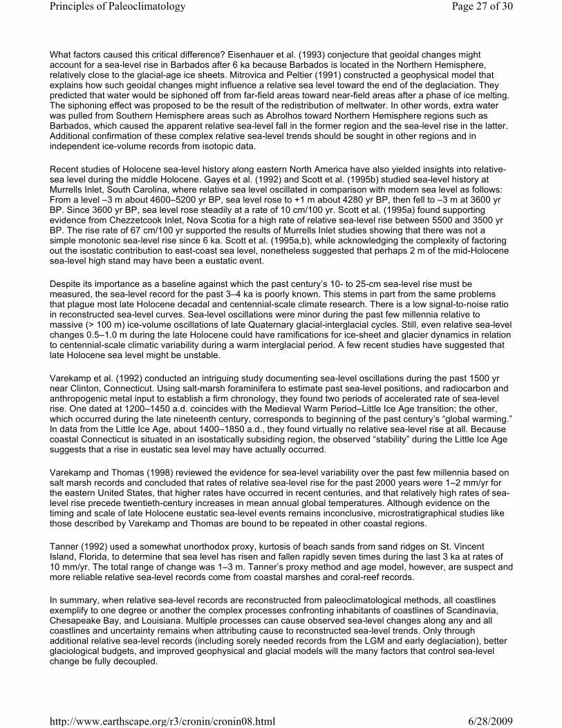
What factors caused this critical difference? Eisenhauer et al. (1993) conjecture that geoidal changes might account for a sea-level rise in Barbados after 6 ka because Barbados is located in the Northern Hemisphere, relatively close to the glacial-age ice sheets. Mitrovica and Peltier (1991) constructed a geophysical model that explains how such geoidal changes might influence a relative sea level toward the end of the deglaciation. They predicted that water would be siphoned off from far-field areas toward near-field areas after a phase of ice melting. The siphoning effect was proposed to be the result of the redistribution of meltwater. In other words, extra water was pulled from Southern Hemisphere areas such as Abrolhos toward Northern Hemisphere regions such as Barbados, which caused the apparent relative sea-level fall in the former region and the sea-level rise in the latter. Additional confirmation of these complex relative sea-level trends should be sought in other regions and in independent ice-volume records from isotopic data.

Recent studies of Holocene sea-level history along eastern North America have also yielded insights into relative-sea level during the middle Holocene. Gayes et al. (1992) and Scott et al. (1995b) studied sea-level history at Murrells Inlet, South Carolina, where relative sea level oscillated in comparison with modern sea level as follows: From a level –3 m about 4600–5200 yr BP, sea level rose to +1 m about 4280 yr BP, then fell to –3 m at 3600 yr BP. Since 3600 yr BP, sea level rose steadily at a rate of 10 cm/100 yr. Scott et al. (1995a) found supporting evidence from Chezzetcook Inlet, Nova Scotia for a high rate of relative sea-level rise between 5500 and 3500 yr BP. The rise rate of 67 cm/100 yr supported the results of Murrells Inlet studies showing that there was not a simple monotonic sea-level rise since 6 ka. Scott et al. (1995a,b), while acknowledging the complexity of factoring out the isostatic contribution to east-coast sea level, nonetheless suggested that perhaps 2 m of the mid-Holocene sea-level high stand may have been a eustatic event.

Despite its importance as a baseline against which the past century’s 10- to 25-cm sea-level rise must be measured, the sea-level record for the past 3–4 ka is poorly known. This stems in part from the same problems that plague most late Holocene decadal and centennial-scale climate research. There is a low signal-to-noise ratio in reconstructed sea-level curves. Sea-level oscillations were minor during the past few millennia relative to massive (> 100 m) ice-volume oscillations of late Quaternary glacial-interglacial cycles. Still, even relative sea-level changes 0.5–1.0 m during the late Holocene could have ramifications for ice-sheet and glacier dynamics in relation to centennial-scale climatic variability during a warm interglacial period. A few recent studies have suggested that late Holocene sea level might be unstable.

Varekamp et al. (1992) conducted an intriguing study documenting sea-level oscillations during the past 1500 yr near Clinton, Connecticut. Using salt-marsh foraminifera to estimate past sea-level positions, and radiocarbon and anthropogenic metal input to establish a firm chronology, they found two periods of accelerated rate of sea-level rise. One dated at 1200–1450 a.d. coincides with the Medieval Warm Period–Little Ice Age transition; the other, which occurred during the late nineteenth century, corresponds to beginning of the past century’s “global warming.” In data from the Little Ice Age, about 1400–1850 a.d., they found virtually no relative sea-level rise at all. Because coastal Connecticut is situated in an isostatically subsiding region, the observed “stability” during the Little Ice Age suggests that a rise in eustatic sea level may have actually occurred.

Varekamp and Thomas (1998) reviewed the evidence for sea-level variability over the past few millennia based on salt marsh records and concluded that rates of relative sea-level rise for the past 2000 years were 1–2 mm/yr for the eastern United States, that higher rates have occurred in recent centuries, and that relatively high rates of sea-level rise precede twentieth-century increases in mean annual global temperatures. Although evidence on the timing and scale of late Holocene eustatic sea-level events remains inconclusive, microstratigraphical studies like those described by Varekamp and Thomas are bound to be repeated in other coastal regions.

Tanner (1992) used a somewhat unorthodox proxy, kurtosis of beach sands from sand ridges on St. Vincent Island, Florida, to determine that sea level has risen and fallen rapidly seven times during the last 3 ka at rates of 10 mm/yr. The total range of change was 1–3 m. Tanner’s proxy method and age model, however, are suspect and more reliable relative sea-level records come from coastal marshes and coral-reef records.

In summary, when relative sea-level records are reconstructed from paleoclimatological methods, all coastlines exemplify to one degree or another the complex processes confronting inhabitants of coastlines of Scandinavia, Chesapeake Bay, and Louisiana. Multiple processes can cause observed sea-level changes along any and all coastlines and uncertainty remains when attributing cause to reconstructed sea-level trends. Only through additional relative sea-level records (including sorely needed records from the LGM and early deglaciation), better glaciological budgets, and improved geophysical and glacial models will the many factors that control sea-level change be fully decoupled.



Historical Sea-Level Change

We conclude this chapter with a brief summary of sea-level history obtained from tide-gauge records of the past few centuries and possible causes of historical sea-level trends. As we have mentioned, sea level has risen approximately 10–25 cm over the past century (Nicholls et al. 1996). Many questions arise from this conclusion. How fast is it rising now? Is the historical rate of rise faster or slower than pre–twentieth century rates? What has caused the historical sea-level rise?

The earliest tide-gauge devices were put in place in Amsterdam in 1682, Venice in 1732, and Stockholm in 1774 (Pirazzoli 1991) to record changing sea level in these early urban centers of Europe. As it became recognized that sea-level change varied from one coastal region to the next, it also became clear that a wider network of sites was needed to evaluate local versus broader sea-level trends. Consequently, more and more tide gauges were established to better quantify sea level. Now the Permanent Service for Mean Sea Level at Bidston Observatory in England maintains a set of 420 tide-gauge records at least 20 years old from which tide-gauge estimates of sea-level change are derived (Raper et al. 1996).

We saw in figure 8-2 the complex tide-gauge records of sea-level history obtained from six regions. The most obvious aspect to this figure is that the trend in each relative sea-level curve is different from the others owing to the many factors that affect relative sea level discussed earlier.

Like many trends derived from monitoring records of climate-related phenomena, sea-level trends obtained from tide gauges suffer from the tradeoff between the length of the record and the geographic coverage available. The longest recorded tide gauges yield longer trends for a particular coast but tell nothing about sea-level change in other regions (Gornitz 1995a,b). Tide gauges in place for the past few decades give a broad spatial coverage (though still predominantly in the Northern Hemisphere) but they cannot be used to establish how sea level varies over longer time scales. Global sea-level trends cannot be established without broad geographic coverage of the world’s coastlines because of the local processes influencing sea level. Consequently, the literature contains estimates of the total sea-level rise over the past century that vary depending on the length and location of the tide-gauge records used.

In recent years, many papers have reconstructed sea level using tide-gauge records in order to better explain the patterns and causes of historical sea-level trends (e.g., Gornitz and Lebedeff 1987; Emery and Aubrey 1991; Douglas 1991; Fletcher 1992; Gornitz 1995b; Warrick et al. 1996; see Raper et al. 1996 for review). By removing the effects of vertical land movements using geological (Gornitz et al. 1995b) and geophysical (Peltier and Tushingham 1989) methods, scientists have reached general agreement on two issues. First, the tide-gauge record is sufficient to evaluate the amount of global sea level only for perhaps the past 60–100 years. Before about 1930, the record is too limited. Second, there is a general consensus that global sea level has been rising along the world’s coasts during the past century. However, estimates of the total sea-level rise and thus the net rate of rise vary widely. For example, Emery and Aubrey (1991) and Nicholls et al. (1996) concluded that total global sea level has risen somewhere between 10–25 cm over the past century. Raper et al. (1996) suggested that, once noise and interannual variations due to oceanographic and atmospheric effects are removed, the range of sea level–rise estimates run from a low of 5 cm to a high of 30 cm for the past century (or 0.5 to 3.0 mm/yr). A rate of 1–2 mm/yr is an oft-cited average rate of rise for the past century (see Douglas 1991, 1992; Gornitz 1995b).

An average rise of sea level of 1 to 2 mm/yr over the past century leads to the question, do historical tide-gauge records offer any evidence for an acceleration in the rate of sea-level rise during the past 100 years. Douglas (1992) studied short and long-term tide-gauge records to address this question. He found that 23 tide-gauge records from 10 different coastal regions for the interval 1905–1985 showed sea level rose at a rate of 0.11 (±0.012) mm/yr. A less extensive tide-gauge data set available for the period 1850–1991 covering a smaller geographical area than the 1905–1985 data set showed that no statistically significant acceleration in the rate of sea-level rise had occurred after 1850. In another study of the rate of recent sea-level rise, Maul and Martin (1993) showed there was likely no acceleration in sea-level rise in the Florida Keys since 1846. Any acceleration in sea-level rise must have preceded the Florida historical records available to them, a point that underscores the need to reconstruct late Holocene sea-level trends from geological evidence.

A similar question might be: is the past century’s rate of sea-level rise rapid compared with rates of sea-level change for the past 2000 years? Varekamp et al. (1992), studying late-Holocene sea level from Connecticut, found



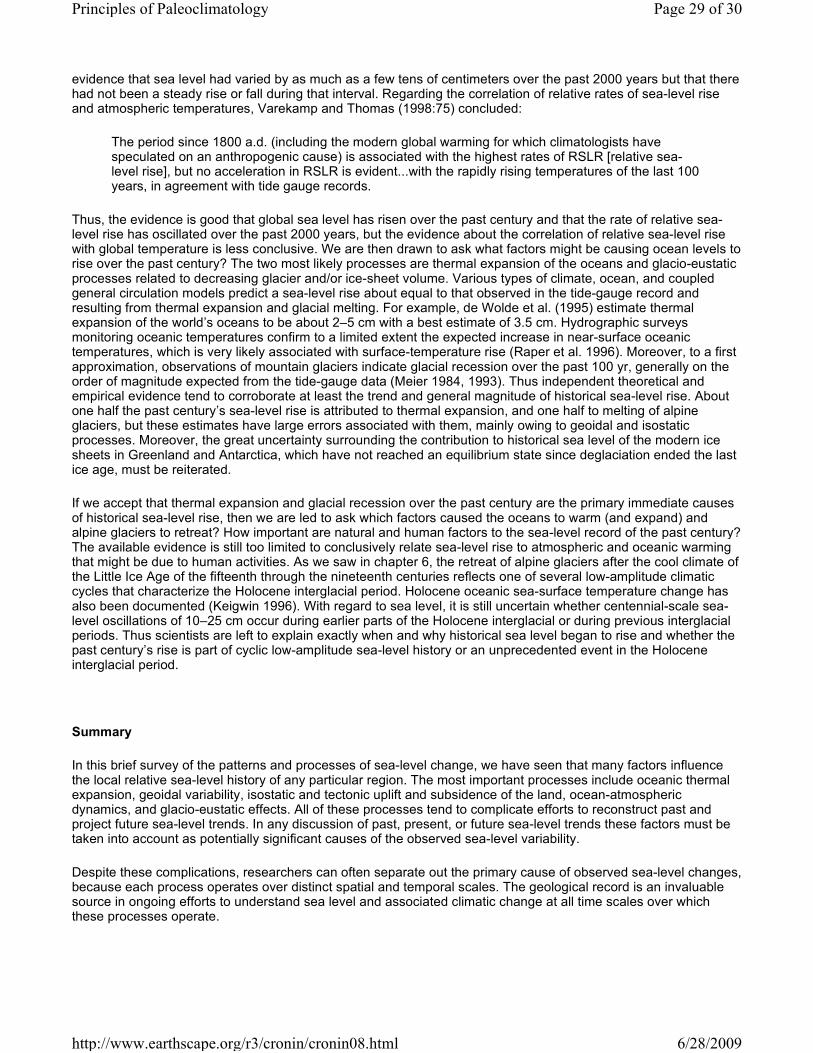
evidence that sea level had varied by as much as a few tens of centimeters over the past 2000 years but that there had not been a steady rise or fall during that interval. Regarding the correlation of relative rates of sea-level rise and atmospheric temperatures, Varekamp and Thomas (1998:75) concluded:

The period since 1800 a.d. (including the modern global warming for which climatologists have speculated on an anthropogenic cause) is associated with the highest rates of RSLR [relative sea-level rise], but no acceleration in RSLR is evident...with the rapidly rising temperatures of the last 100 years, in agreement with tide gauge records.

Thus, the evidence is good that global sea level has risen over the past century and that the rate of relative sea-level rise has oscillated over the past 2000 years, but the evidence about the correlation of relative sea-level rise with global temperature is less conclusive. We are then drawn to ask what factors might be causing ocean levels to rise over the past century? The two most likely processes are thermal expansion of the oceans and glacio-eustatic processes related to decreasing glacier and/or ice-sheet volume. Various types of climate, ocean, and coupled general circulation models predict a sea-level rise about equal to that observed in the tide-gauge record and resulting from thermal expansion and glacial melting. For example, de Wolde et al. (1995) estimate thermal expansion of the world’s oceans to be about 2–5 cm with a best estimate of 3.5 cm. Hydrographic surveys monitoring oceanic temperatures confirm to a limited extent the expected increase in near-surface oceanic temperatures, which is very likely associated with surface-temperature rise (Raper et al. 1996). Moreover, to a first approximation, observations of mountain glaciers indicate glacial recession over the past 100 yr, generally on the order of magnitude expected from the tide-gauge data (Meier 1984, 1993). Thus independent theoretical and empirical evidence tend to corroborate at least the trend and general magnitude of historical sea-level rise. About one half the past century’s sea-level rise is attributed to thermal expansion, and one half to melting of alpine glaciers, but these estimates have large errors associated with them, mainly owing to geoidal and isostatic processes. Moreover, the great uncertainty surrounding the contribution to historical sea level of the modern ice sheets in Greenland and Antarctica, which have not reached an equilibrium state since deglaciation ended the last ice age, must be reiterated.

If we accept that thermal expansion and glacial recession over the past century are the primary immediate causes of historical sea-level rise, then we are led to ask which factors caused the oceans to warm (and expand) and alpine glaciers to retreat? How important are natural and human factors to the sea-level record of the past century? The available evidence is still too limited to conclusively relate sea-level rise to atmospheric and oceanic warming that might be due to human activities. As we saw in chapter 6, the retreat of alpine glaciers after the cool climate of the Little Ice Age of the fifteenth through the nineteenth centuries reflects one of several low-amplitude climatic cycles that characterize the Holocene interglacial period. Holocene oceanic sea-surface temperature change has also been documented (Keigwin 1996). With regard to sea level, it is still uncertain whether centennial-scale sea-level oscillations of 10–25 cm occur during earlier parts of the Holocene interglacial or during previous interglacial periods. Thus scientists are left to explain exactly when and why historical sea level began to rise and whether the past century’s rise is part of cyclic low-amplitude sea-level history or an unprecedented event in the Holocene interglacial period.

Summary

In this brief survey of the patterns and processes of sea-level change, we have seen that many factors influence the local relative sea-level history of any particular region. The most important processes include oceanic thermal expansion, geoidal variability, isostatic and tectonic uplift and subsidence of the land, ocean-atmospheric dynamics, and glacio-eustatic effects. All of these processes tend to complicate efforts to reconstruct past and project future sea-level trends. In any discussion of past, present, or future sea-level trends these factors must be taken into account as potentially significant causes of the observed sea-level variability.

Despite these complications, researchers can often separate out the primary cause of observed sea-level changes, because each process operates over distinct spatial and temporal scales. The geological record is an invaluable source in ongoing efforts to understand sea level and associated climatic change at all time scales over which these processes operate.



Principles of Paleoclimatology: Perspectives in Paleobiology and Earth History



8. sea-level change - florida gulf coast...

Documents