8 nonlinear dynamics of nanomechanical resonatorsronlif/pubs/wiley-ch8-2010.pdf · 2013-05-06 ·...
TRANSCRIPT
221
8Nonlinear Dynamics of Nanomechanical ResonatorsRon Lifshitz and M.C. Cross
8.1Nonlinearities in NEMS and MEMS Resonators
In the last decade we have witnessed exciting technological advances in the fabri-cation and control of microelectromechanical and nanoelectromechanical systems(MEMS & NEMS) [16, 19, 26, 54, 55]. Such systems are being developed for a host ofnanotechnological applications, such as highly sensitive mass [25, 34, 67], spin [56],and charge detectors [17, 18], as well as for basic research in the mesoscopic physicsof phonons [63], and the general study of the behavior of mechanical degrees offreedom at the interface between the quantum and the classical worlds [5, 64]. Sur-prisingly, MEMS & NEMS have also opened up a whole new experimental windowinto the study of the nonlinear dynamics of discrete systems in the form of nonlin-ear micromechanical and nanomechanical oscillators and resonators.
The purpose of this review is to provide an introduction to the nonlinear dynam-ics of micromechanical and nanomechanical resonators that starts from the basics,but also touches upon some of the advanced topics that are relevant for current ex-periments with MEMS & NEMS devices. We begin in this section with a generalmotivation, explaining why nonlinearities are so often observed in NEMS & MEMSdevices. In Section 8.2 we describe the dynamics of one of the simplest nonlineardevices, the Duffing resonator, while giving a tutorial in secular perturbation the-ory as we calculate its response to an external drive. We continue to use the sameanalytical tools in Section 8.3 to discuss the dynamics of a parametrically-excitedDuffing resonator, building up to the description of the dynamics of an array ofcoupled parametrically-excited Duffing resonators in Section 8.4. We conclude inSection 8.5 by giving an amplitude equation description for the array of coupledDuffing resonators, allowing us to extend our analytic capabilities in predictingand explaining the nature of its dynamics.
Nonlinear Dynamics of Nanosystems. Edited by Günter Radons, Benno Rumpf, and Heinz Georg SchusterCopyright © 2010 WILEY-VCH Verlag GmbH & Co. KGaA, WeinheimISBN: 978-3-527-40791-0
222 8 Nonlinear Dynamics of Nanomechanical Resonators
8.1.1Why Study Nonlinear NEMS and MEMS?
Interest in the nonlinear dynamics of microelectromechanical and nanoelectrome-chanical systems (MEMS & NEMS) has grown rapidly over the last few years, driv-en by a combination of practical needs as well as fundamental questions. Nonlinearbehavior is readily observed in micro- and nanoscale mechanical devices [1, 2, 9–12, 19, 24, 27, 30, 33, 50, 57, 61, 62, 66, 68, 71, 72]. Consequently, there exists apractical need to understand this behavior in order to avoid it when it is unwanted,and exploit it efficiently when it is wanted. At the same time, advances in the fab-rication, transduction, and detection of MEMS & NEMS resonators has opened upan exciting new experimental window into the study of fundamental questions innonlinear dynamics. Typical nonlinear MEMS & NEMS resonators are character-ized by extremely high frequencies, recently going beyond 1 GHz [15, 32, 48], andrelatively weak dissipation, with quality factors in the range of 102–104. For suchdevices the regime of physical interest is that of steady state motion, as transientstend to disappear before they are detected. This, and the fact that weak dissipationcan be treated as a small perturbation, provide a great advantage for quantitativetheoretical study. Moreover, the ability to fabricate arrays of tens to thousands ofcoupled resonators opens new possibilities in the study of nonlinear dynamics ofintermediate numbers of degrees of freedom, much larger than one can study inmacroscopic or tabletop experiments, yet much smaller than one studies whenconsidering nonlinear aspects of phonon dynamics in a crystal.
The collective response of coupled arrays might be useful for signal enhance-ment and noise reduction [21, 22], as well as for sophisticated mechanical signalprocessing applications. Such arrays have already exhibited interesting nonlineardynamics, ranging from the formation of extended patterns [8, 38], as one com-monly observes in analogous continuous systems such as Faraday waves, to thatof intrinsically localized modes [39, 58–60]. Thus, nanomechanical resonator ar-rays are perfect for testing dynamical theories of discrete nonlinear systems withmany degrees of freedom. At the same time, the theoretical understanding of suchsystems may prove useful for future nanotechnological applications.
8.1.2Origin of Nonlinearity in NEMS and MEMS Resonators
We are used to thinking about mechanical resonators as being simple harmonicoscillators, acted upon by linear elastic forces that obey Hooke’s law. This is usuallya very good approximation, as most materials can sustain relatively large deforma-tions before their intrinsic stress-strain relation breaks away from a simple lineardescription. Nevertheless, one commonly encounters nonlinear dynamics in mi-cromechanical and nanomechanical resonators long before the intrinsic nonlinearregime is reached. Most evident are nonlinear effects that enter the equation ofmotion in the form of a force that is proportional to the cube of the displacementαx3. These turn a simple harmonic resonator with a linear restoring force into
8.1 Nonlinearities in NEMS and MEMS Resonators 223
a so-called Duffing resonator. The two main origins of the observed nonlinear ef-fects are illustrated below with the help of two typical examples. These are due tothe effect of external potentials that are often nonlinear, and geometric effects thatintroduce nonlinearities even though the individual forces that are involved are alllinear. The Duffing nonlinearity αx3 can be positive, assisting the linear restoringforce, making the resonator stiffer, and increasing its resonance frequency. It canalso be negative, working against the linear restoring force, making the resonatorsofter, and decreasing its resonance frequency. The two examples we give below il-lustrate how both of these situations can arise in realistic MEMS & NEMS devices.
Additional sources of nonlinearity may be found in experimental realizations ofMEMS and NEMS resonators due to practical reasons. These may include non-linearities in the actuation and in the detection mechanisms that are used for in-teracting with the resonators. There could also be nonlinearities that result fromthe manner in which the resonator is clamped by its boundaries to the surround-ing material. These all introduce external factors that may contribute to the overallnonlinear behavior of the resonator.
Finally, nonlinearities often appear in the damping mechanisms that accompanyevery physical resonator. We shall avoid going into the detailed description of thevariety of physical processes that govern the damping of a resonator. Suffice it tosay that whenever it is reasonable to expand the forces acting on a resonator up tothe cube of the displacement x3, it should correspondingly be reasonable to addto the linear damping, which is proportional to the velocity of the resonator Px , anonlinear damping term of the form x2 Px , which increases with the amplitude ofmotion. Such nonlinear damping will be considered in our analysis below.
8.1.3Nonlinearities Arising from External Potentials
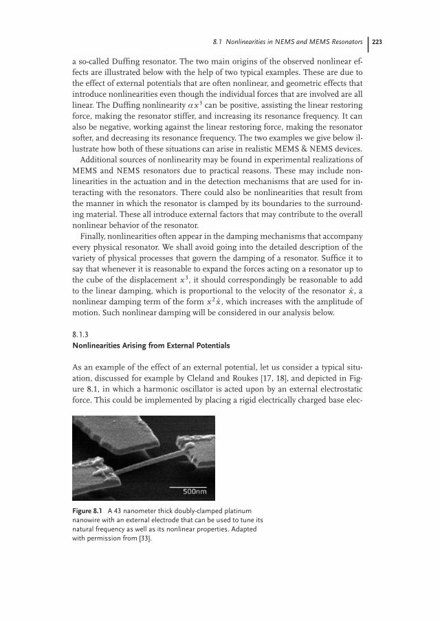
As an example of the effect of an external potential, let us consider a typical situ-ation, discussed for example by Cleland and Roukes [17, 18], and depicted in Fig-ure 8.1, in which a harmonic oscillator is acted upon by an external electrostaticforce. This could be implemented by placing a rigid electrically charged base elec-
Figure 8.1 A 43 nanometer thick doubly-clamped platinumnanowire with an external electrode that can be used to tune itsnatural frequency as well as its nonlinear properties. Adaptedwith permission from [33].
224 8 Nonlinear Dynamics of Nanomechanical Resonators
trode near an oppositely charged NEMS or MEMS resonator. If the equilibriumseparation between the resonator and the base electrode in the absence of electriccharge is d, the deviation away from this equilibrium position is denoted by X,the effective elastic spring constant of the resonator is K, and the charge q on theresonator is assumed to be constant, then the potential energy of the resonator isgiven by
V(X ) D 12
K X 2 C
d C X. (8.1)
In SI units C D Aq2/4π0, where A is a numerical factor of order unity that takesinto account the finite dimensions of the charged resonator and base electrode.The new equilibrium position X0 in the presence of charge can be determined bysolving the cubic equation
dV
dXD K X C C
(d C X )2D 0 . (8.2)
If we now expand the potential acting on the resonator in a power series in thedeviation x D X X0 from this new equilibrium, we obtain
V(x ) ' V(X0) C 12
K 2C
(d C X0)3
x2 C C
(d C X0)4 x3 C
(d C X0)5 x4
D V(X0) C 12
k x2 C 13
x3 C 14
αx4 .
(8.3)
This gives rise, without any additional driving or damping, to an equation of mo-tion of the form
m Rx C kx C x2 C αx3 D 0 , with > 0, α < 0 , (8.4)
where m is the effective mass of the resonator and k is its new effective spring con-stant, which is softened by the electrostatic attraction to the base electrode. Notethat if 2C/(d C X0)3 > K , the electrostatic force exceeds the elastic restoring forceand the resonator is pulled onto the base electrode. is a positive symmetry break-ing quadratic elastic constant that pulls the resonator towards the base electroderegardless of the sign of x, and α is the cubic, or Duffing, elastic constant that, ow-ing to its negative sign, softens the effect of the linear restoring force. It should besufficient to stop the expansion here, unless the amplitude of the motion is muchlarger than the size of the resonator, or if by some coincidence the effects of thequadratic and cubic nonlinearities happen to cancel each other out, a situation thatwill become clearer after reading Section 8.2.3.
8.1.4Nonlinearities Due to Geometry
As an illustration of how nonlinearities can emerge from linear forces due to ge-ometric effects, consider a doubly-clamped thin elastic beam, which is one of the
8.1 Nonlinearities in NEMS and MEMS Resonators 225
most commonly encountered NEMS resonators. Because of the clamps at bothends, as the beam deflects in its transverse motion it necessarily stretches. As longas the amplitude of the transverse motion is much smaller than the width of thebeam, this effect can be neglected. But with NEMS beams it is often the case thatthey are extremely thin, and are driven quite strongly, making it common for theamplitude of vibration to exceed the width. Let us consider this effect in somedetail by starting with the Euler-Bernoulli equation, which is the commonly usedapproximate equation of motion for a thin beam [43]. For a transverse displacementX(z, t) from equilibrium, which is much smaller than the length L of the beam,the equation is
S@2 X
@t2 D E I@4 X
@z4 C T@2 X
@z2 , (8.5)
where z is the coordinate along the length of the beam is the mass density, S
is the area of the cross section of the beam, E is the Young’s modulus, I is themoment of inertia, and T the tension in the beam. The latter is composed of itsinherent tension T0 and the additional tension ∆T due to bending that inducesan extension ∆L in the length of the beam. Inherent tension results from the factthat in equilibrium in the doubly-clamped configuration, the actual length of thebeam may differ from its rest length, being either extended (positive T0) or com-pressed (negative T0). The additional tension ∆T is given by the strain, or relativeextension of the beam ∆L/L, multiplied by Young’s modulus E and the area of thebeam’s cross section S. For small displacements, the total length of the beam canbe expanded as
L C ∆L DZ L
0dz
s1 C
@X
@z
2
' L C 12
Z L
0dz
@X
@z
2
. (8.6)
The equation of motion (8.5) then clearly becomes nonlinear
S@2 X
@t2 D E I@4 X
@z4 C"
T0 C E S
2L
Z L
0dz
@X
@z
2#
@2 X
@z2 . (8.7)
We can treat this equation perturbatively [49, 69]. We first consider the linearpart of the equation, which has the form of (8.5) with T0 in place of T, separate thevariables,
Xn(z, t) D xn(t)φn(z) , (8.8)
and find its spatial eigenmodes φn(z). For the eigenmodes, we use the conventionthat the local maximum of the eigenmode φn(z) that is nearest to the center of thebeam is scaled to 1. Thus xn(t) measures the actual deflection of the beam at thepoint nearest to its center that extends the furthest. Next, we assume that the beamis vibrating predominantly in one of these eigenmodes and use this assumption toevaluate the effective Duffing parameter αn , multiplying the x3
n term in the equa-tion of motion for this mode. Corrections to this approximation will appear only at
226 8 Nonlinear Dynamics of Nanomechanical Resonators
higher orders of xn . We multiply (8.7) by the chosen eigenmode φn(z) and inte-grate over z to get, after some integration by parts, a Duffing equation of motionfor the amplitude of the nth mode xn(t),
Rxn C"
E I
S
Rφ00
n2dzR
φ2n dz
C T0
S
Rφ0
n2dzR
φ2n dz
#xn C
264 E
2L
Rφ0
n2dz
2
Rφ2
n dz
375 x3
n D 0 ,
(8.9)
where primes denote derivatives with respect to z, and all the integrals are from0 to L. Note that we have obtained a positive Duffing term, indicating a stiffeningnonlinearity, as opposed to the softening nonlinearity that we saw in the previoussection. Also note that the effective spring constant can be made negative by com-pressing the equilibrium beam, thus making T0 large and negative. This may leadto the so-called Euler instability, which is a buckling instability of the beam.
To evaluate the effective Duffing nonlinearity αn for the nth mode, we introducea dimensionless parameter Oαn by rearranging the equation of motion (8.9) to havethe form
Rxn C ω2n xn
1 C Oαn
x2n
d2
D 0 , (8.10)
where ωn is the normal frequency of the nth mode, d is the width or diameter ofthe beam in the direction of the vibration, and xn is the maximum displacementof the beam near its center. This parameter can then be evaluated regardless of theactual dimension of the beam.
In the limit of small residual tension T0, the eigenmodes are those dominatedby bending given by [43]
φn(z) D 1an
[(sin kn L sinh kn L) (cos kn z cosh kn z)
(cos kn L cosh kn L) (sin kn z sinh kn z)] , (8.11)
where an is the value of the function in the square brackets at its local maximumthat is closest to z D 0.5, and the wave vectors kn are solutions of the transcenden-tal equation cos kn L cosh kn L D 1. The first few values are
fkn Lg ' f4.7300, 7.8532, 10.9956, 14.1372, 17.2788, 20.4204 . . .g , (8.12)
and the remaining ones tend towards odd-integer multiples of π/2 as n increases.Using these eigenfucntions, we can obtain explicit values for the dimensionlessDuffing parameters for the different modes by calculating
Oαn D S d2
2I
1L
Rφ02
n dz2
1L
Rφ00
n2 dz
S d2
2IOn . (8.13)
The first few values aren On
o' f0.1199, 0.2448, 0.3385, 0.3706, 0.3908, 0.4068, 0.4187, . . .g , (8.14)
8.2 The Directly-Driven Damped Duffing Resonator 227
tending to an asymptotic value of 1/2 as n ! 1. For beams with rectangular orcircular cross sections, the geometric prefactor evaluates to
S d2
2ID
(16 Circular cross section ,
6 Rectangular cross section .(8.15)
Thus the dimensionless Duffing parameters are of order 1, and therefore the signif-icance of the nonlinear behavior is solely determined by the ratio of the deflectionto the width of the beam.
In the limit of large equilibrium tension, the beam essentially behaves as a stringwith relatively negligible resistance to bending. The eigenmodes are those of astring,
φn(z) D sin nπ
Lz
, n D 1, 2, 3 . . . , (8.16)
and, if we denote the equilibrium extension of the beam as ∆L0 D LT0/E S , thedimensionless Duffing parameters are exactly given by
Oαn D d2
2∆L0
Zφ0
n2 dz D (nπd)2
4L∆L0. (8.17)
In the large tension limit, as in the case of a string, the dimensionless Duffingparameters are proportional to the inverse aspect ratio of the beam d/L times theratio between its width and the extension from its rest length d/∆L0, at least one ofwhich can be a very small parameter. For this reason nonlinear effects are relativelynegligible in these systems.
8.2The Directly-Driven Damped Duffing Resonator
8.2.1The Scaled Duffing Equation of Motion
Let us begin by considering a single nanomechanical Duffing resonator with linearand nonlinear damping that is driven by an external sinusoidal force. We shallstart with the common situation where there is symmetry between x and x, andconsider the changes that are introduced by adding symmetry-breaking terms later.Such a resonator is described by the equation of motion
md2 Qxd Qt2
C Γd Qxd Qt C mω2
0 Qx C Qα Qx3 C Qη Qx2 d Qxd Qt D QG cos Qω Qt , (8.18)
where m is its effective mass, k D mω20 is its effective spring constant, Qα is the
cubic spring constant or Duffing parameter, Γ is the linear damping rate, and Qη isthe coefficient of nonlinear damping – damping that increases with the amplitude
228 8 Nonlinear Dynamics of Nanomechanical Resonators
of oscillation. We follow the convention that physical parameters that are to beimmediately rescaled appear with twiddles, as the first step in dealing with such anequation is to scale away as many unnecessary parameters as possible, leaving onlythose that are physically significant. This then removes all of the twiddles. We doso by: (1) Measuring time in units of ω1
0 so that the dimensionless time variableis t D ω0 Qt. (2) Measuring amplitudes of motion in units of length for which aunit-amplitude oscillation doubles the frequency of the resonator. This is achieved
by taking the dimensionless length variable to be x D Qxq
Qα/mω20. For the doubly-
clamped beam of width or diameter d, discussed in Section 8.1.4, this length isx D Qxp Oαn/d. (3) Dividing the equation by an overall factor of ω3
0
pm3/ Qα. This
yields a scaled Duffing equation of the form
Rx C Q1 Px C x C x3 C ηx2 Px D G cos ω t , (8.19)
where dots denote derivatives with respect to the dimensionless time t, all the di-mensionless parameters are related to the physical ones by
Q1 D Γmω0
, η D Qηω0
Qα , G DQG
ω30
r Qαm3 , and ω D Qω
ω0, (8.20)
and Q is the quality factor of the resonator.
8.2.2A Solution Using Secular Perturbation Theory
We proceed to calculate the response of the damped Duffing resonator to an ex-ternal sinusoidal drive, as given by (8.19), by making use of secular perturbationtheory [31, 65]. We do so in the limit of a weak linear damping rate Q1, whichwe use to define a small expansion parameter, Q1 1. In most actual ap-plications, Q is at least on the order of 100, making this limit well-justified. Wealso consider the limit of weak oscillations where it is justified to truncate the ex-pansion of the force acting on the resonator at the third power of x. We do so byrequiring that the cubic force x3 be a factor of smaller than the linear force, orequivalently, by requiring the deviation from equilibrium x to be on the order ofp
. We ensure that the external driving force has the right strength to induce suchweak oscillations by having it enter the equation at the same order as all the otherphysical effects. This, in effect, requires the amplitude of the drive to be G D 3/2g.To see why, recall that for a regular linear resonance, x is proportional to G Q. Q isof order 1 and we want x to be of order
p, and so G must be of order 3/2. Final-
ly, since damping is weak we expect to see a response only close to the resonancefrequency. We therefore take the driving frequency to be of the form ω D 1 C Ω .The equation of motion (8.19) thus becomes
Rx C Px C x C x3 C ηx2 Px D 3/2g cos(1 C Ω )t . (8.21)
This is the equation we shall study using secular perturbation theory, while occa-sionally comparing the results with the original physical equation (8.18).
8.2 The Directly-Driven Damped Duffing Resonator 229
With the expectation that the motion of the resonator far from equilibrium willbe on the order of 1/2, we try a solution of the form
x (t) Dp
2
A(T ) eit C c.c.
C 3/2x1(t) C . . . (8.22)
where c.c. denotes complex conjunction.The lowest order contribution to this solution is based on the solution to the lin-
ear equation of motion of a simple harmonic oscillator (SHO) Rx C x D 0, whereT D t is a slow time variable, allowing the complex amplitude A(T ) to vary slowlyin time due to the effect of all the other terms in the equation. As we shall im-mediately see, the slow temporal variation of A(T ) also allows us to ensure thatthe perturbative correction x1(t) as well as all higher-order corrections to the linearequation do not diverge, as they do if one uses naive perturbation theory. Using therelation
PA D dA
dtD
dA
dT A0 , (8.23)
we calculate the time derivatives of the trial solution (8.22)
Px Dp
2
iA C A0
eit C c.c.
C 3/2 Px1(t) C . . . (8.24a)
Rx Dp
2
A C 2 iA0 C 2A00
eit C c.c. C 3/2 Rx1(t) C . . . (8.24b)
By substituting these expressions back into the equation of motion (8.21) and pick-ing out all terms of order 3/2, we get for the first perturbative correction
Rx1 Cx1 D
iA0 i12
A 3 C iη8
jAj2A C g
2eiΩ T
eit 1 C iη
8A3 e3it Cc.c.
(8.25)
The collection of terms proportional to eit on the right-hand side of (8.25), calledthe secular terms, act like a force that drives the SHO on the left-hand side exactlyat its resonance frequency. The sum of all these terms must therefore vanish so thatthe perturbative correction x1(t) will not diverge. This requirement is the so-called“solvability condition”, giving us an equation for determining the slowly varyingamplitude A(T ),
dA
dTD 1
2A C i
38
jAj2A η8
jAj2A ig
2eiΩ T . (8.26)
This general equation could be used to study many different effects [20]. Here weuse it to study the steady-state dynamics of the driven Duffing resonator.
We ignore initial transients and assume that there exists a steady-state solutionof the form
A(T ) D a eiΩ T jaj eiφ eiΩ T . (8.27)
230 8 Nonlinear Dynamics of Nanomechanical Resonators
With this expression for the slowly varying amplitude A(T ), the solution to theoriginal equation of motion (8.21) becomes an oscillation at the drive frequencyω D 1 C Ω ,
x (t) D 1/2jaj cos(ω t C φ) C O(3/2) , (8.28)
where we are not interested in the actual correction x1(t) of order 3/2, but ratherin finding the fixed complex amplitude a of the lowest order term. This amplitudea can be any solution of the equation
34
jaj2 2Ω
C i
1 C η4
jaj2
a D g , (8.29)
obtained by substituting the steady-state solution (8.27) into Eq. (8.26) of the secularterms.
The magnitude and phase of the response are then given explicitly by
jaj2 D g22Ω 3
4 jaj22 C 1 C 1
4 ηjaj22 (8.30a)
and
tan φ D 1 C 14 ηjaj2
2Ω 34 jaj2 . (8.30b)
By reintroducing the original physical scales, we can obtain the physical solution tothe original equations of motion Qx ( Qt) ' Qx0 cos( Qω Qt C φ), where Qx0 D jajpΓω0/ Qα,and therefore
Qx20 D
QG
2mω20
2
Qωω0
ω0 3
8Qα
mω20
Qx20
2 C
12 Q1 C 1
8Qη
mω0Qx2
0
2 (8.31a)
and
tan φ DΓ2 C Qη
8 Qx20
m Qω mω0 3 Qα8ω0
Qx20
. (8.31b)
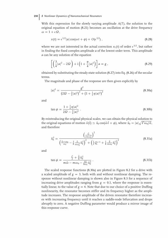
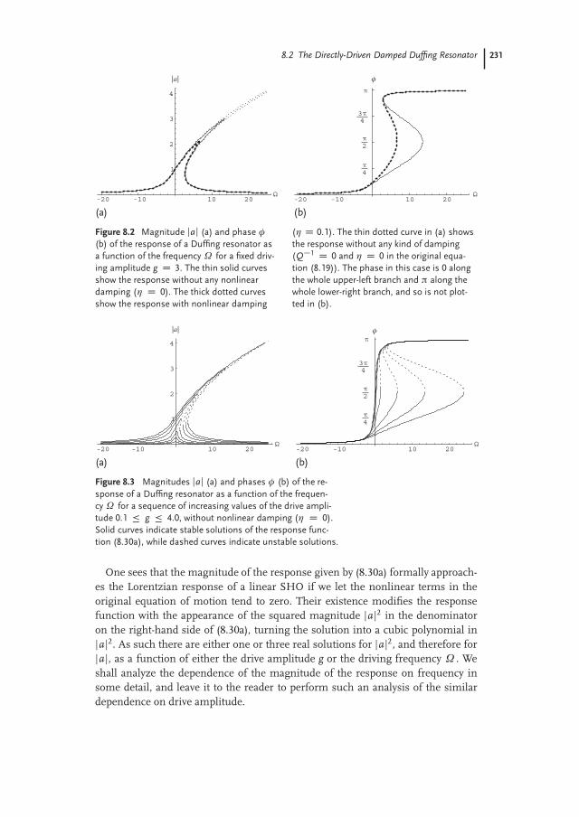
The scaled response functions (8.30a) are plotted in Figure 8.2 for a drive witha scaled amplitude of g D 3, both with and without nonlinear damping. The re-sponse without nonlinear damping is shown also in Figure 8.3 for a sequence ofincreasing drive amplitudes ranging from g D 0.1, where the response is essen-tially linear, to the value of g D 4. Note that due to our choice of a positive Duffingnonlinearity, the resonator becomes stiffer and its frequency higher as the ampli-tude increases. The response amplitude of the driven resonator therefore increas-es with increasing frequency until it reaches a saddle-node bifurcation and dropsabruptly to zero. A negative Duffing parameter would produce a mirror image ofthis response curve.
8.2 The Directly-Driven Damped Duffing Resonator 231
-20 -10 10 20
1
2
3
4
|a| φ
-20 -10 10 20
π2
3π4
π
π4
(a) (b)
Figure 8.2 Magnitude jaj (a) and phase φ(b) of the response of a Duffing resonator asa function of the frequency Ω for a fixed driv-ing amplitude g D 3. The thin solid curvesshow the response without any nonlineardamping (η D 0). The thick dotted curvesshow the response with nonlinear damping
(η D 0.1). The thin dotted curve in (a) showsthe response without any kind of damping(Q1 D 0 and η D 0 in the original equa-tion (8.19)). The phase in this case is 0 alongthe whole upper-left branch and π along thewhole lower-right branch, and so is not plot-ted in (b).
-20 -10 10 20Ω
1
2
3
4
|a|
-20 -10 10 20
φ
π2
3π4
π
π4
(a) (b)
Figure 8.3 Magnitudes jaj (a) and phases φ (b) of the re-sponse of a Duffing resonator as a function of the frequen-cy Ω for a sequence of increasing values of the drive ampli-tude 0.1 g 4.0, without nonlinear damping (η D 0).Solid curves indicate stable solutions of the response func-tion (8.30a), while dashed curves indicate unstable solutions.
One sees that the magnitude of the response given by (8.30a) formally approach-es the Lorentzian response of a linear SHO if we let the nonlinear terms in theoriginal equation of motion tend to zero. Their existence modifies the responsefunction with the appearance of the squared magnitude jaj2 in the denominatoron the right-hand side of (8.30a), turning the solution into a cubic polynomial injaj2. As such there are either one or three real solutions for jaj2, and therefore forjaj, as a function of either the drive amplitude g or the driving frequency Ω . Weshall analyze the dependence of the magnitude of the response on frequency insome detail, and leave it to the reader to perform such an analysis of the similardependence on drive amplitude.
232 8 Nonlinear Dynamics of Nanomechanical Resonators
In order to analyze the magnitude of the response jaj as a function of drivingfrequency Ω , we differentiate the response function (8.30a), resulting in 3
64
9 C η2 jaj4 C 1
4 (η 6Ω ) jaj2 C 14 C Ω 2 djaj2
D 34 jaj4 2Ω jaj2 dΩ . (8.32)
This allows us immediately to find the condition for resonance, where the mag-nitude of the response is at its peak, by requiring that djaj2/dΩ D 0. We findthat the resonance frequency Ωmax depends quadratically on the peak magnitudejajmax, according to
Ωmax D 38 jaj2max , (8.33a)
or in terms of the original variables as
Qωmax D ω0 C 38
αmω0
( Qx0)2max . (8.33b)
The curve satisfying (8.33a), for which jaj D p8Ω /3, is plotted in Figure 8.3. It
forms a square root backbone that connects all the resonance peaks for the differ-ent driving amplitudes, which is often seen in typical experiments with nanome-chanical resonators. Thus, the peak of the response is pulled further toward higherfrequencies as the driving amplitude g is increased, as expected from a stiffeningnonlinearity.
When the drive amplitude g is sufficiently strong, we can use Eq. (8.32) to findthe two saddle-node bifurcation points, where the number of solutions changesfrom one to three and then back from three to one. At these points dΩ /djaj2 D 0,yielding a quadratic equation in Ω whose solutions are
Ω ˙SN D 3
4 jaj2 ˙ 12
q316 (3 η2) jaj4 ηjaj2 1 . (8.34)
When the two solutions are real, corresponding to the two bifurcation points, alinear stability analysis shows that the upper and lower branches of the responseare stable solutions and the middle branch that exists for Ω
SN < Ω < Ω CSN is
unstable. When the drive amplitude g is reduced, it approaches a critical value gc
where the two bifurcation points merge into an inflection point. At this point bothdΩ /djaj2 D 0 and d2Ω /(djaj2)2 D 0, providing two equations for determining thecritical condition for the onset of bistability, or the existence of two stable solutionbranches,
jaj2c D 83
1p3 η
, Ωc D 1
2p
3
3p
3 C ηp3 η
, gc2 D 32
279 C η2p
3 η3 . (8.35)
For the case without nonlinear damping, η D 0, the critical values are jaj2c D(4/3)3/2 and Ωc D (3/4)1/2, for which the critical drive amplitude is gc D (4/3)5/4.For 0 < η <
p3, the critical driving amplitude gc that is required for having
bistability increases with η, as shown in Figure 8.4. For η >p
3 the discriminantin Eq. (8.34) is always negative, prohibiting the existence of bistability of solutions.
8.2 The Directly-Driven Damped Duffing Resonator 233
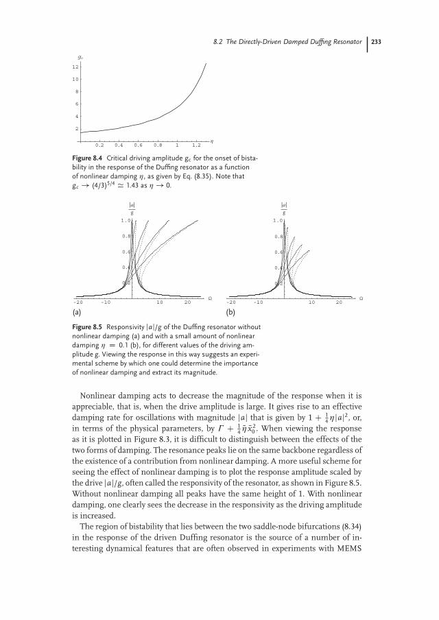
0.2 0.4 0.6 0.8 1.21
2
4
6
8
10
12
gc
Figure 8.4 Critical driving amplitude gc for the onset of bista-bility in the response of the Duffing resonator as a functionof nonlinear damping η, as given by Eq. (8.35). Note thatgc ! (4/3)5/4 ' 1.43 as η ! 0.
-20 -10 10 20Ω
0.2
0.4
0.6
0.8
1.0 1.0
-20 -10 10 20
0.2
0.4
0.6
0.8
(a) (b)
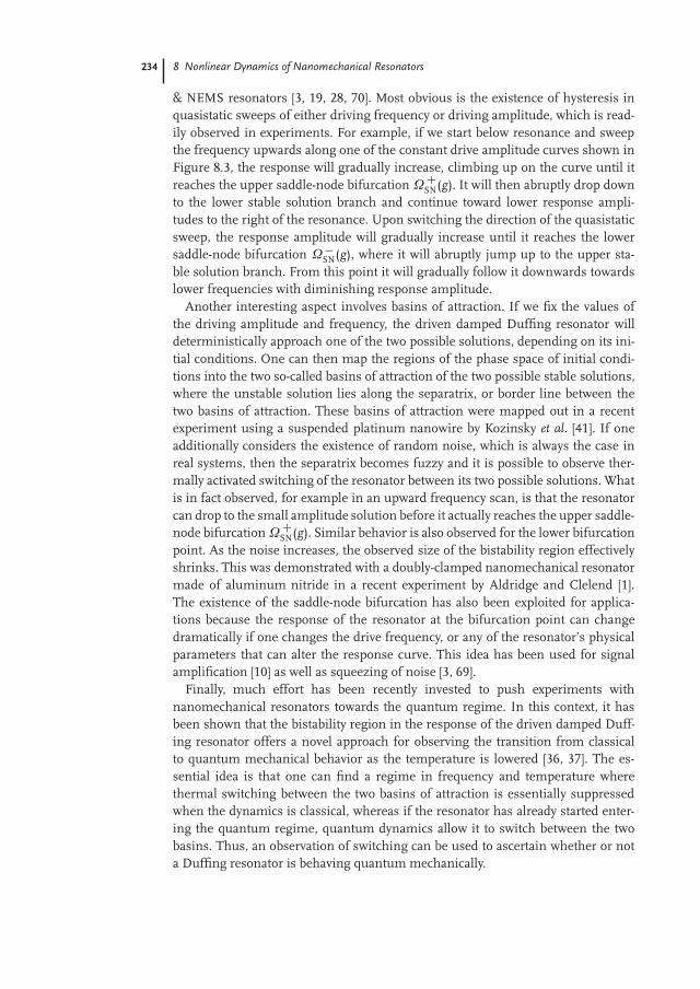
|a|g
|a|g
Figure 8.5 Responsivity jaj/g of the Duffing resonator withoutnonlinear damping (a) and with a small amount of nonlineardamping η D 0.1 (b), for different values of the driving am-plitude g. Viewing the response in this way suggests an experi-mental scheme by which one could determine the importanceof nonlinear damping and extract its magnitude.
Nonlinear damping acts to decrease the magnitude of the response when it isappreciable, that is, when the drive amplitude is large. It gives rise to an effectivedamping rate for oscillations with magnitude jaj that is given by 1 C 1
4 ηjaj2, or,in terms of the physical parameters, by Γ C 1
4 Qη Qx20 . When viewing the response
as it is plotted in Figure 8.3, it is difficult to distinguish between the effects of thetwo forms of damping. The resonance peaks lie on the same backbone regardless ofthe existence of a contribution from nonlinear damping. A more useful scheme forseeing the effect of nonlinear damping is to plot the response amplitude scaled bythe drive jaj/g, often called the responsivity of the resonator, as shown in Figure 8.5.Without nonlinear damping all peaks have the same height of 1. With nonlineardamping, one clearly sees the decrease in the responsivity as the driving amplitudeis increased.
The region of bistability that lies between the two saddle-node bifurcations (8.34)in the response of the driven Duffing resonator is the source of a number of in-teresting dynamical features that are often observed in experiments with MEMS
234 8 Nonlinear Dynamics of Nanomechanical Resonators
& NEMS resonators [3, 19, 28, 70]. Most obvious is the existence of hysteresis inquasistatic sweeps of either driving frequency or driving amplitude, which is read-ily observed in experiments. For example, if we start below resonance and sweepthe frequency upwards along one of the constant drive amplitude curves shown inFigure 8.3, the response will gradually increase, climbing up on the curve until itreaches the upper saddle-node bifurcation Ω C
SN(g). It will then abruptly drop downto the lower stable solution branch and continue toward lower response ampli-tudes to the right of the resonance. Upon switching the direction of the quasistaticsweep, the response amplitude will gradually increase until it reaches the lowersaddle-node bifurcation Ω
SN(g), where it will abruptly jump up to the upper sta-ble solution branch. From this point it will gradually follow it downwards towardslower frequencies with diminishing response amplitude.
Another interesting aspect involves basins of attraction. If we fix the values ofthe driving amplitude and frequency, the driven damped Duffing resonator willdeterministically approach one of the two possible solutions, depending on its ini-tial conditions. One can then map the regions of the phase space of initial condi-tions into the two so-called basins of attraction of the two possible stable solutions,where the unstable solution lies along the separatrix, or border line between thetwo basins of attraction. These basins of attraction were mapped out in a recentexperiment using a suspended platinum nanowire by Kozinsky et al. [41]. If oneadditionally considers the existence of random noise, which is always the case inreal systems, then the separatrix becomes fuzzy and it is possible to observe ther-mally activated switching of the resonator between its two possible solutions. Whatis in fact observed, for example in an upward frequency scan, is that the resonatorcan drop to the small amplitude solution before it actually reaches the upper saddle-node bifurcation Ω C
SN(g). Similar behavior is also observed for the lower bifurcationpoint. As the noise increases, the observed size of the bistability region effectivelyshrinks. This was demonstrated with a doubly-clamped nanomechanical resonatormade of aluminum nitride in a recent experiment by Aldridge and Clelend [1].The existence of the saddle-node bifurcation has also been exploited for applica-tions because the response of the resonator at the bifurcation point can changedramatically if one changes the drive frequency, or any of the resonator’s physicalparameters that can alter the response curve. This idea has been used for signalamplification [10] as well as squeezing of noise [3, 69].
Finally, much effort has been recently invested to push experiments withnanomechanical resonators towards the quantum regime. In this context, it hasbeen shown that the bistability region in the response of the driven damped Duff-ing resonator offers a novel approach for observing the transition from classicalto quantum mechanical behavior as the temperature is lowered [36, 37]. The es-sential idea is that one can find a regime in frequency and temperature wherethermal switching between the two basins of attraction is essentially suppressedwhen the dynamics is classical, whereas if the resonator has already started enter-ing the quantum regime, quantum dynamics allow it to switch between the twobasins. Thus, an observation of switching can be used to ascertain whether or nota Duffing resonator is behaving quantum mechanically.
8.2 The Directly-Driven Damped Duffing Resonator 235
8.2.3Addition of Other Nonlinear Terms
It is worth considering the addition of other nonlinear terms that were not includ-ed in our original equation of motion (8.18). Without increasing the order of thenonlinearity, we could still add quadratic symmetry breaking terms of the form x2,x Px , and Px2 as well as additional cubic damping terms of the form Px3 and x Px2.Such terms may appear naturally in actual physical situations, like the examplesdiscussed in Section 8.1.2. For the reader who wishes to skip to the following sec-tion on parametrically-driven Duffing resonators, we state at the outset that theaddition of such terms does not alter the response curves that we described in theprevious section in any fundamental way. They merely conspire to renormalize theeffective values of the coefficients used in the original equation of motion. Thus,without any particular model at hand, it is difficult to discern the existence of suchterms in the equation.
Consider an equation like (8.18), but with additional terms of the form givenabove,
md2 Qxd Qt2
C Γd Qxd Qt C mω2
0 Qx C Q Qx2 C Qµ Qx d Qxd Qt C Q
d Qxd Qt
2
C Qα Qx3 C Qη Qx2 d QxdQt
C Qν Qx
d Qxd Qt
2
C Q
d Qxd Qt
3
D QG cos Qω Qt , (8.36)
and then perform the same scaling as in (8.20) for the additional parameters, pro-ducing
DQ
ω0p
m Qα , µ D Qµpm Qα , D Qω0p
m Qα , ν D Qνω20
Qα , DQ ω3
0
Qα .
(8.37)
After performing the same scaling as before with the small parameter D Q1,this yields a scaled equation of motion with all the additional nonlinearities,
Rx C Px C x C x2 C µx Px C Px2 C x3 C ηx2 Px C νx Px2 C Px3 D 3/2g cos ω t .
(8.38)
The important difference between this equation and the one we solved earlier (8.21)is that with a similar scaling of x with
p, we now have terms on the order of . We
therefore need to modify our trial expansion to contain such terms as well, yielding
x (t) D px0(t, T ) C x1/2(t, T ) C 3/2x1(t, T ) C . . . , (8.39)
with x0 D 12
A(T ) eit C c.c.
as before.
We begin by collecting all terms on the order of , arriving at
Rx1/2 C x1/2 D 12 ( C ) jAj2 1
4
( C iµ) A2 e2it C c.c.
. (8.40)
236 8 Nonlinear Dynamics of Nanomechanical Resonators
This equation for the first correction x1/2(t) contains no secular terms, and there-fore can be solved immediately to give
x1/2(t) D 12 ( C ) jAj2 C 1
12
( C iµ) A2 e2it C c.c.
. (8.41)
We substitute this solution into the ansatz (8.39) and back into the equation of mo-tion (8.38), and proceed by collecting terms on the order of 3/2. We find a numberof additional terms of this order that did not appear earlier on the right-hand sideof (8.25) for the correction x1(t),
2x0x1/2 µx0 Px1/2 C Px0x1/2
2 Px0 Px1/2 νx0 Px20 Px3
0
D ˚ 512 ( C ) C 1
6 2 C 124 µ2 1
8 ν C i
18 µ ( C ) 3
8 jAj2A eit
C nonsecular terms .
(8.42)
After adding the additional secular terms, we obtain a modified equation for theslowly varying amplitude A(T ),
dA
dTD 1
2A C i
38
1 10
9 ( C ) 4
92 1
9µ2 C 1
3ν
jAj2A
18
(η µ ( C ) C 3 ) jAj2A ig
2eiΩ T
12
A C i38
αeffjAj2A 18
ηeffjAj2A ig
2eiΩ T . (8.43)
We find that the equation is formally identical to the previous result (8.26) beforeadding the extra nonlinear terms. The response curves and the discussion of theprevious section therefore still apply after taking into account all of the quadraticand cubic nonlinear terms. All of these terms combine in a particular way, givingrise to the two effective cubic parameters defined in (8.43). This, in fact, allows onesome flexibility in tuning the nonlinearities of a Duffing resonator in real experi-mental situations. For example, Kozinsky et al. [40] use this flexibility to tune theeffective Duffing parameter αeff via an external electrostatic potential, as describedin Section 8.1.3 and shown in Figure 8.1. This affects both the quadratic parameterQ and the cubic parameter Qα in the physical equation of motion (8.36). Note thatdue to the different signs of the various contributions to the effective nonlinear pa-rameters, one could actually cause the cubic terms to vanish, altering the responsein a fundamental way.
8.3Parametric Excitation of a Damped Duffing Resonator
Parametric excitation offers an alternative approach for actuating MEMS or NEMSresonators. Instead of applying an external force that acts directly on the resonator,one modulates one or more of its physical parameters as a function of time, which
8.3 Parametric Excitation of a Damped Duffing Resonator 237
in turn modulates the normal frequency of the resonator. This is what happenson a swing when the up-and-down motion of the center of mass of the swingingchild effectively changes the length of the swing, thereby modulating its naturalfrequency. The most effective way to swing is to move the center of mass up anddown twice in every period of oscillation, but one can also swing by moving upand down at slower rates, namely once every nth multiple of half a period, for anyinteger n.
Let H be the relative amplitude by which the normal frequency is modulated, andωP be the frequency of the modulation, often called the pump frequency. One canshow [42] that there is a sequence of tongue shaped regions in the H ωP planewhere the smallest fluctuations away from the quiescent state of the swing, or anyother parametrically-excited resonator [66], are exponentially amplified. This hap-pens when the amplitude of the modulation H is sufficiently strong to overcomethe effect of damping, where the threshold for the nth instability tongue scales as(Q1)1/n . Above this threshold, the amplitude of the motion grows until it is sat-urated by nonlinear effects. We shall describe the nature of these oscillations fordriving above threshold later, both for the first (n D 1) and the second (n D 2)instability tongues, but first we shall consider the dynamics when the driving am-plitude is just below threshold, as it also offers interesting behavior and a possi-bility for novel applications such as parametric amplification [4, 12, 57] and noisesqueezing [57].
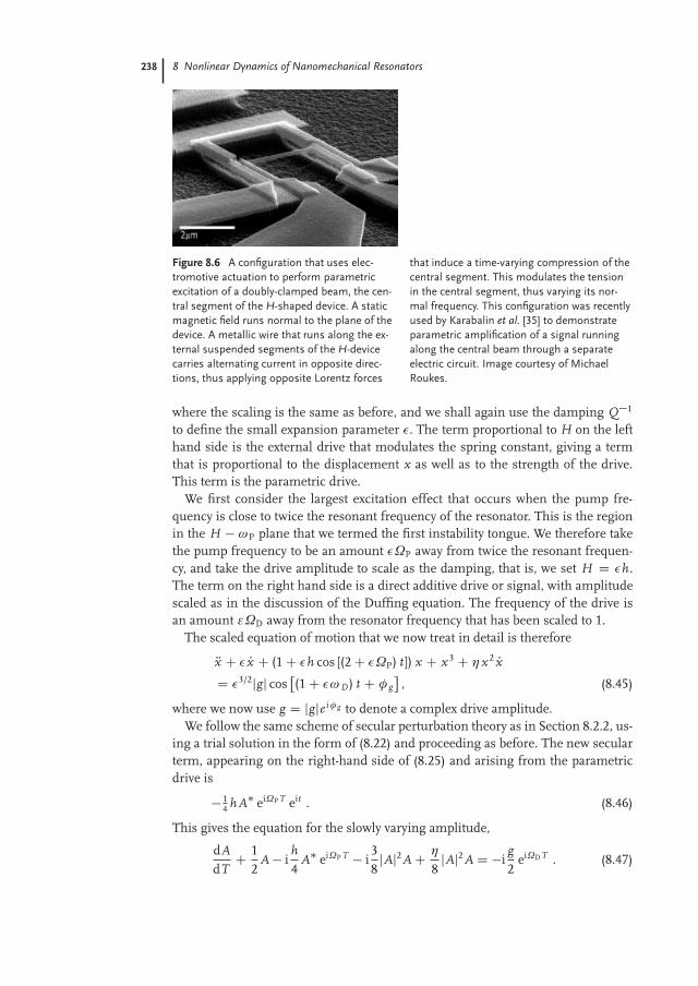
There are a number of actual schemes for the realization of parametric excita-tion in MEMS & NEMS devices. The simplest and probably most commonly usedon the micron scale is to use an external electrode that can induce an external po-tential. If the external potential is modulated in time it can change the effectivespring constant of the resonator [24, 51, 52, 66, 71, 72]. Based on our treatment ofthis situation in Section 8.1.3, this method is likely to modulate all the coefficientsin the potential felt by the resonator, thus also modulating, for example, the Duff-ing parameter α. Similarly, one may devise configurations in which an externalelectrode deflects a doubly-clamped beam from its equilibrium, thereby inducingextra tension within the beam itself that can be modulated in time, as describedin Section 8.1.4. Alternatively, one may generate motion in the clamps holding adoubly-clamped beam by its ends, thus inducing in it a time-varying tension whichis likely to affect the other physical parameters to a lesser extent. An example of thismethod is shown in Figure 8.6. These methods allow one to modulate the tensionin the beam directly and thus modulate its normal frequency. More recently, Mas-manidis et al. [45] developed layered piezoelectric NEMS structures whose tensioncan be fine tuned in doubly-clamped configurations, thus enabling fine control ofthe normal frequency of the beam with a simple turn of a knob.
Only a minor change is required in our equation of the driven damped Duffingresonator to accommodate this new situation, namely the addition of a modula-tion of the linear spring constant. Beginning with the scaled form of the Duffingequation (8.19), we obtain
Rx C Q1 Px C [1 C H cos ωP t] x C x3 C ηx2 Px D G cosωD t C φ g
, (8.44)
238 8 Nonlinear Dynamics of Nanomechanical Resonators
Figure 8.6 A configuration that uses elec-tromotive actuation to perform parametricexcitation of a doubly-clamped beam, the cen-tral segment of the H-shaped device. A staticmagnetic field runs normal to the plane of thedevice. A metallic wire that runs along the ex-ternal suspended segments of the H-devicecarries alternating current in opposite direc-tions, thus applying opposite Lorentz forces
that induce a time-varying compression of thecentral segment. This modulates the tensionin the central segment, thus varying its nor-mal frequency. This configuration was recentlyused by Karabalin et al. [35] to demonstrateparametric amplification of a signal runningalong the central beam through a separateelectric circuit. Image courtesy of MichaelRoukes.
where the scaling is the same as before, and we shall again use the damping Q1
to define the small expansion parameter . The term proportional to H on the lefthand side is the external drive that modulates the spring constant, giving a termthat is proportional to the displacement x as well as to the strength of the drive.This term is the parametric drive.
We first consider the largest excitation effect that occurs when the pump fre-quency is close to twice the resonant frequency of the resonator. This is the regionin the H ωP plane that we termed the first instability tongue. We therefore takethe pump frequency to be an amount ΩP away from twice the resonant frequen-cy, and take the drive amplitude to scale as the damping, that is, we set H D h.The term on the right hand side is a direct additive drive or signal, with amplitudescaled as in the discussion of the Duffing equation. The frequency of the drive isan amount εΩD away from the resonator frequency that has been scaled to 1.
The scaled equation of motion that we now treat in detail is therefore
Rx C Px C (1 C h cos [(2 C ΩP) t]) x C x3 C ηx2 PxD 3/2jgj cos
(1 C ωD ) t C φ g
, (8.45)
where we now use g D jgje i φg to denote a complex drive amplitude.We follow the same scheme of secular perturbation theory as in Section 8.2.2, us-
ing a trial solution in the form of (8.22) and proceeding as before. The new secularterm, appearing on the right-hand side of (8.25) and arising from the parametricdrive is
14 hA eiΩP T eit . (8.46)
This gives the equation for the slowly varying amplitude,
dA
dTC 1
2A i
h
4A eiΩP T i
38
jAj2A C η8
jAj2A D ig
2eiΩD T . (8.47)
8.3 Parametric Excitation of a Damped Duffing Resonator 239
8.3.1Driving Below Threshold: Amplification and Noise Squeezing
We first study the amplitude of the response of a parametrically-pumped Duffingresonator to an external direct drive g ¤ 0. We will see that the characteristic be-havior changes from amplification of an applied signal to oscillations at a criticalvalue of h D hc D 2, even in the absence of a signal. It is therefore convenientto introduce a reduced parametric drive Nh D h/ hc D h/2 that plays the role ofa bifurcation parameter with a critical value of 1. We begin by assuming that thedrive is small enough so that the magnitude of the response remains small and thenonlinear terms in (8.47) can be neglected. This gives the linear equation
dA
dTC 1
2A i
Nh2
A eiΩP T D ig
2eiΩD T . (8.48)
In general, at long times after transients have died out, the solution will take theform
A D a0 eiΩD T C b0 ei(ΩPΩD)T , (8.49)
where a0 and b0 are complex constants.We first consider the degenerate case where the pump frequency is tuned such
that it is always twice the signal frequency. In this case ΩP D 2ΩD, and the longtime solution is
A D a eiΩD T (8.50)
with a a time independent complex amplitude. Substituting this into (8.48) gives
(2ΩD i)a Nha D g . (8.51)
Equation (8.51) is easily solved. If we first look on resonance, ΩD D 0, we find
a D eiπ/4
"cos(φg C π/4)
(1 Nh)C i
sin(φg C π/4)
(1 C Nh)
#jgj , (8.52)
where we remind the reader that g D jgj eiφg so that φg measures the phase of thesignal relative to the pump. Equation (8.52) shows that on resonance and for Nh ! 1(or h ! hc D 2), the strongest enhancement of the response occurs for a signal thathas a phase π/4 relative to the pump. Physically, this means that the maximumof the signal occurs a quarter of a pump cycle after a maximum of the pump. (Thephase 3π/4 gives the same result: this corresponds to shifting the oscillations bya complete pump period.) The enhancement diverges as Nh ! 1, provided that thesignal amplitude g is small enough that the enhanced response remains within thelinear regime. For a fixed signal amplitude g, the response will become large asNh ! 1, so that the nonlinear terms in (8.47) must be retained and the expressionswe have derived no longer hold. This situation is discussed in the next section.
240 8 Nonlinear Dynamics of Nanomechanical Resonators
On the other hand, there is a weak suppression, by a factor of 2 as Nh ! 1, fora signal that has a relative phase π/4 or 5π/4. The latter pertains to the case of asignal maximum that occurs a quarter of a pump cycle before a maximum of thepump. A noise signal on the right-hand side of the equation of motion (8.45) wouldhave both phase components. This leads to the squeezing of the noisy displacementdriven by this noise, with the response at phase π/4 amplified and the responseat phase π/4 quenched.
The full expression for ΩD ¤ 0 for the response amplitude is
a D "
2ΩD C (i C Nh e2 iφg )
4Ω 2D C (1 Nh2)
#g . (8.53)
For Nh ! 1 the response is large when ΩD 1, that is, for frequencies much closerto resonance than the original width of the resonator response. In these limits thefirst term in the numerator may be neglected unless φg ' π/4. This then gives
jaj D 2ˇg cos(φg C π/4)
ˇ4Ω 2
D C (1 Nh2). (8.54)
This is not the same as the expression for a resonant response, since the frequencydependence of the amplitude, not amplitude squared, is Lorentzian. However, es-timating a quality factor from the width of the sharp peak would give an enhanced
quality factor / 1/p
1 Nh2, becoming very large as Nh ! 1. For the case φg D π/4the magnitude of the response is
ˇaφgDπ/4
ˇ Dq
4Ω 2D C (1 Nh)2
4Ω 2D C (1 Nh2)
jNgj . (8.55)
This initially increases as the frequency approaches resonance, but decreases for
ΩD .p
1 Nh, approaching jgj /2 for ΩD ! 0, Nh ! 1.For the general or nondegenerate case of ΩP ¤ 2ΩD, it is straightforward to
repeat the calculation with the ansatz (8.49). The result is
a0 D 2(ΩP ΩD) C i
4ΩD(ΩP ΩD) 2i(ΩP 2ΩD) C 1 Nh2g . (8.56)
Notice that this does not reduce to (8.53) for ΩP D 2ΩD, since we miss some of theinterference terms in the degenerate case if we base the calculation on ΩP ¤ 2ΩD.Also, of course, there is no dependence of the magnitude of the response on thephase of the signal φg, since for different frequencies the phase difference cannotbe defined independent of an arbitrary choice of the origin of time. If the pumpfrequency is maintained fixed at twice the resonator resonance frequency, corre-sponding to ΩP D 0, the expression for the amplitude of the response simplifiesto
a0 D 2ΩD i
4Ω 2D C 4 iΩD C 1 Nh2
g . (8.57)
8.3 Parametric Excitation of a Damped Duffing Resonator 241
-2 -1 1 2ΩD
5
10
15
20
Response
-2 -1 1 2
2
4
6
8
10
Response
(a) (b)
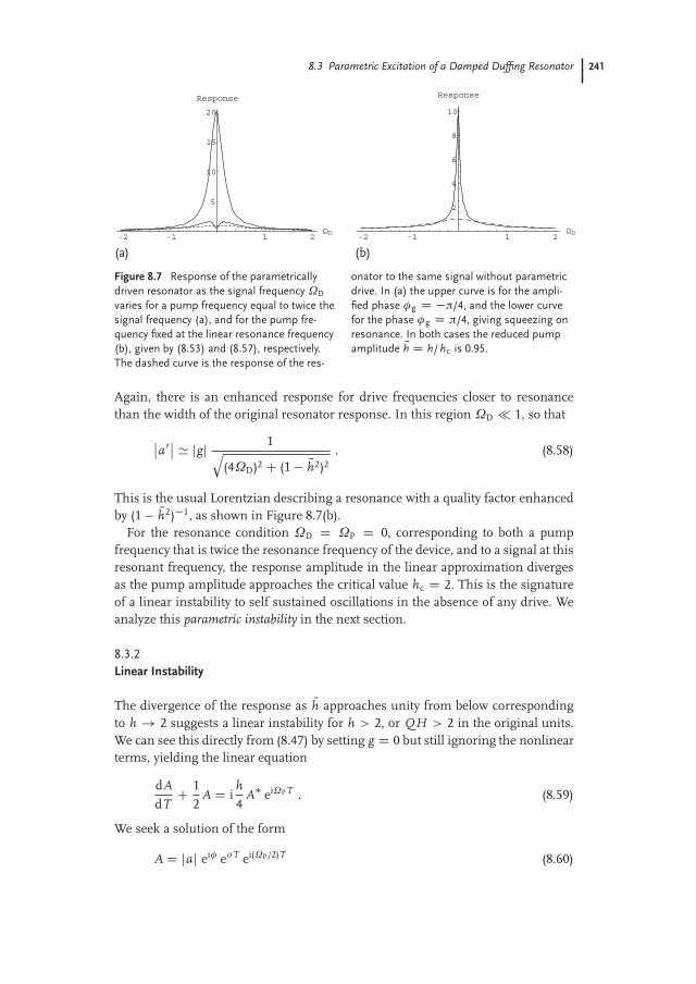
Figure 8.7 Response of the parametricallydriven resonator as the signal frequency ΩDvaries for a pump frequency equal to twice thesignal frequency (a), and for the pump fre-quency fixed at the linear resonance frequency(b), given by (8.53) and (8.57), respectively.The dashed curve is the response of the res-
onator to the same signal without parametricdrive. In (a) the upper curve is for the ampli-fied phase φg D π/4, and the lower curvefor the phase φg D π/4, giving squeezing onresonance. In both cases the reduced pumpamplitude Nh D h/ hc is 0.95.
Again, there is an enhanced response for drive frequencies closer to resonancethan the width of the original resonator response. In this region ΩD 1, so that
ˇa0
ˇ ' jgj 1q(4ΩD)2 C (1 Nh2)2
. (8.58)
This is the usual Lorentzian describing a resonance with a quality factor enhancedby (1 Nh2)1, as shown in Figure 8.7(b).
For the resonance condition ΩD D ΩP D 0, corresponding to both a pumpfrequency that is twice the resonance frequency of the device, and to a signal at thisresonant frequency, the response amplitude in the linear approximation divergesas the pump amplitude approaches the critical value hc D 2. This is the signatureof a linear instability to self sustained oscillations in the absence of any drive. Weanalyze this parametric instability in the next section.
8.3.2Linear Instability
The divergence of the response as Nh approaches unity from below correspondingto h ! 2 suggests a linear instability for h > 2, or QH > 2 in the original units.We can see this directly from (8.47) by setting g D 0 but still ignoring the nonlinearterms, yielding the linear equation
dA
dTC 1
2A D i
h
4A eiΩP T . (8.59)
We seek a solution of the form
A D jaj eiφ eσT ei(ΩP/2)T (8.60)
242 8 Nonlinear Dynamics of Nanomechanical Resonators
Γ= 0
Γ=0
Ω
/
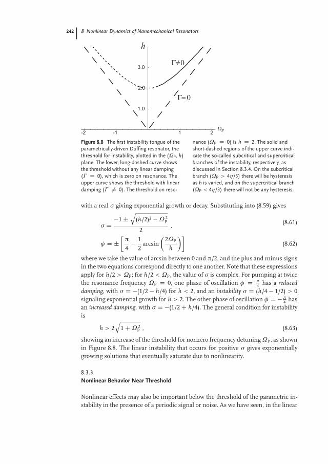
Figure 8.8 The first instability tongue of theparametrically-driven Duffing resonator, thethreshold for instability, plotted in the (ΩP, h)plane. The lower, long-dashed curve showsthe threshold without any linear damping(Γ D 0), which is zero on resonance. Theupper curve shows the threshold with lineardamping (Γ ¤ 0). The threshold on reso-
nance (ΩP D 0) is h D 2. The solid andshort-dashed regions of the upper curve indi-cate the so-called subcritical and supercriticalbranches of the instability, respectively, asdiscussed in Section 8.3.4. On the subcriticalbranch (ΩP > 4η/3) there will be hysteresisas h is varied, and on the supercritical branch(ΩP < 4η/3) there will not be any hysteresis.
with a real σ giving exponential growth or decay. Substituting into (8.59) gives
σ D1 ˙
q(h/2)2 Ω 2
P
2, (8.61)
φ D ˙
π4
12
arcsin
2ΩP
h
(8.62)
where we take the value of arcsin between 0 and π/2, and the plus and minus signsin the two equations correspond directly to one another. Note that these expressionsapply for h/2 > ΩP; for h/2 < ΩP, the value of σ is complex. For pumping at twicethe resonance frequency ΩP D 0, one phase of oscillation φ D π
4 has a reduced
damping, with σ D (1/2 h/4) for h < 2, and an instability σ D (h/4 1/2) > 0signaling exponential growth for h > 2. The other phase of oscillation φ D π
4 hasan increased damping, with σ D (1/2 C h/4). The general condition for instabilityis
h > 2q
1 C Ω 2P , (8.63)
showing an increase of the threshold for nonzero frequency detuning ΩP, as shownin Figure 8.8. The linear instability that occurs for positive σ gives exponentiallygrowing solutions that eventually saturate due to nonlinearity.
8.3.3Nonlinear Behavior Near Threshold
Nonlinear effects may also be important below the threshold of the parametric in-stability in the presence of a periodic signal or noise. As we have seen, in the linear
8.3 Parametric Excitation of a Damped Duffing Resonator 243
approximation the gain below threshold diverges as h ! hc. This is unphysical,and for a given signal or noise strength there is some h close enough to hc wherenonlinear saturation of the gain will become important. This will give a smooth be-havior of the response of the driven system as h passes through hc into the unstableregime. We first analyze the effects of nonlinearity near the threshold of the insta-bility, and calculate the smooth behavior as h passes through hc in the presence ofan applied signal. In the following section we study the effects of nonlinearity onthe self-sustained oscillations above threshold with more generality.
We take h to be close to hc, and we take the signal to be small. This introducesa second level of “smallness”. We have already assumed that the damping and thedeviation of the pump frequency from resonance are both small. This means thatthe critical parametric drive Hc is also small. We now assume that jH Hcj is smallcompared with Hc, or, equivalently in scaled units, that jh hcj is small comparedwith hc. We then introduce the perturbation parameter δ to implement this, thatis, we assume that
δ D h hc
hc 1 . (8.64)
We now use the same type of secular perturbation theory as the method leadingto (8.47) to develop the expansion in δ. For simplicity we will develop the theory forthe most interesting case of resonant pump and signal frequencies ΩP D ΩD D 0.The critical value of h is then hc D 2, and the solution to (8.47) that becomesmarginally stable at this value is
A D b eiπ/4 , (8.65)
with b a real constant.For h near hc we make the ansatz for the solution
A D δ1/2b0(τ) eiπ/4 C δ3/2b1(τ) C , (8.66)
where b0 is a real function of τ D δT . The latter is a new and even slower timescale that determines the time variation of the real amplitude b0 near threshold.We must also assume that the signal amplitude is very small, that is, g D δ3/2 Og, intotal yielding G D (δ)3/2 Og. Substituting (8.66) into (8.47) and collecting terms atO(δ3/2) yields
12
(b1 b1 ) D Og
2eiπ/4 db0
dτC 1
2b0 C i
38
b30 η
8b3
0 . (8.67)
The left-hand side of this equation is necessarily imaginary, so in order to havea solution for b1 such that the perturbation expansion is valid, the real part ofthe right-hand side must be zero. This is the solvability condition for the secularperturbation theory. This gives
db0
dτD 1
2b0 η
8b3
0 j Ogj2
cos(φg C π/4) . (8.68)
244 8 Nonlinear Dynamics of Nanomechanical Resonators
It is more informative to write this equation in terms of the the variables withoutthe δ scaling. Introducing the “unscaled” amplitude b D δ1/2b0 and generaliz-ing (8.65) such that
A D b eiπ/4 C O(δ3/2) , (8.69)
we can write the equation as
db
dTD 1
2h hc
hcb η
8b3 jgj
2cos(φg C π/4) . (8.70)
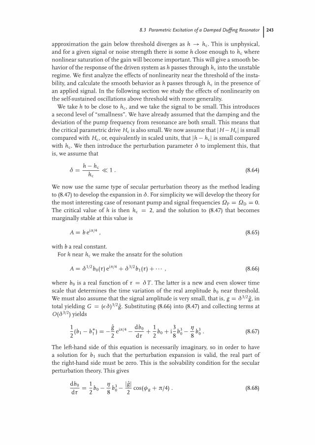
Equation (8.70) can be used to investigate many phenomena, such as transientsabove threshold, and how the amplitude of the response to a signal varies as h pass-es through the instability threshold. The unphysical divergence of the response toa small signal as h ! hc from below is now eliminated. For example, exactly atthreshold h D hc we have
jbj D
4η
ˇg cos(φg C π/4)
ˇ1/3
, (8.71)
giving a finite response, but one proportional to jgj1/3 rather than to jgj. The gainjb/gj scales as jgj2/3 for h D hc, and gets smaller as the signal gets larger, asshown in Figure 8.9. Note that the physical origin of the saturation at the lowestorder of perturbation theory is nonlinear damping. Without nonlinear dampingthe response amplitude (8.71) still diverges. With linear damping that is still small,one would need to go to higher orders of perturbation theory to find a differentphysical mechanism that can provide this kind of saturation. The response to noisecan also be investigated by replacing the jgj cos(φg Cπ/4) drive by a noise function.Equation (8.70) and the noisy version appear in many contexts of phase transitionsand bifurcations, and so solutions are readily found in the literature [20].
-0.1 -0.05 0.05(h-hc)/hc
0.1
0.2
Response
(a)-0.1 -0.05 0.05
10
100
1000
Gain
(h-hc)/hc
(b)
Figure 8.9 Saturation of the response b (a) and gainˇb/g
ˇ(b)
as the parametric drive h passes through the critical value hc,for four different signal levels g. The signal levels are
pη/4
times 102.5, 103, 103.5, and 104, increasing upwards forthe response figure, and downwards for the gain figure. Theresponse amplitude is also measured in units of
pη/4. The
phase of the signal is φg D π/4.
8.3 Parametric Excitation of a Damped Duffing Resonator 245
8.3.4Nonlinear Saturation above Threshold
The linear instability leads to exponential growth of the amplitude, regardless ofthe signal, and results in its saturation. In order to understand this process, weneed to return to the full nonlinear treatment of (8.47) with g D 0. Ignoring initialtransients and assuming that the nonlinear terms in the equation are sufficient tosaturate the growth of the instability, we try a steady-state solution of the form
A(T ) D aei
ΩP2
T . (8.72)
This amplitude a can be any solution of the equation34
jaj2 ΩP
C i
1 C η
4jaj2
a D h
2a , (8.73)
obtained by substituting the steady-state solution (8.72) into the equation of the sec-ular terms (8.47). We immediately see that having no response (a D 0) is always apossible solution regardless of the excitation frequency ΩP. Expressing a D jaj eiφ
and taking the magnitude squared of both sides, we obtain the intensity jaj2 of thenontrivial response as all positive roots of the equation
ΩP 34
jaj22
C
1 C η4
jaj22 D h2
4. (8.74)
In addition to the solution jaj D 0, we have a quadratic equation for jaj2 andtherefore, at most, two additional positive solutions for jaj. This has the form ofa distorted ellipse in the (ΩP, jaj2) plane and a parabola in the (jaj2, h) plane. Inaddition, we obtain for the relative phase of the response
φ D i2
lna
aD 1
2arctan
1 C η4 jaj2
34 jaj2 ΩP
. (8.75)
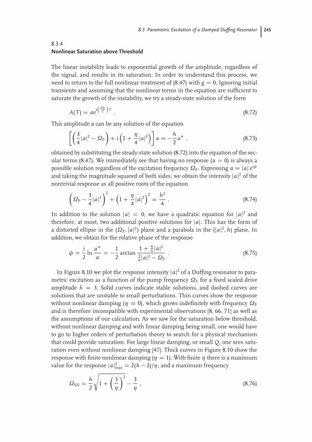
In Figure 8.10 we plot the response intensity jaj2 of a Duffing resonator to para-metric excitation as a function of the pump frequency ΩP for a fixed scaled driveamplitude h D 3. Solid curves indicate stable solutions, and dashed curves aresolutions that are unstable to small perturbations. Thin curves show the responsewithout nonlinear damping (η D 0), which grows indefinitely with frequency ΩP
and is therefore incompatible with experimental observations [8, 66, 71] as well asthe assumptions of our calculation. As we saw for the saturation below threshold,without nonlinear damping and with linear damping being small, one would haveto go to higher orders of perturbation theory to search for a physical mechanismthat could provide saturation. For large linear damping, or small Q, one sees satu-ration even without nonlinear damping [47]. Thick curves in Figure 8.10 show theresponse with finite nonlinear damping (η D 1). With finite η there is a maximumvalue for the response jaj2max D 2(h 2)/η, and a maximum frequency
ΩSN D h
2
s1 C
3η
2
3η
, (8.76)
246 8 Nonlinear Dynamics of Nanomechanical Resonators
-1 1 2
0.4
0.8
1.2
1.6
2.02h 4
P
Figure 8.10 Response intensity jaj2 as a function of the pumpfrequency ΩP, for fixed amplitude h D 3. Solid curves are stablesolutions; dashed curves are unstable solutions. Thin curvesshow the response without nonlinear damping (η D 0). Thickcurves show the response for finite nonlinear damping (η D 1).Dotted lines indicate the maximal response intensity jaj2max andthe saddle-node frequency ΩSN.
at a saddle-node bifurcation, where the stable and unstable nontrivial solutionsmeet. For frequencies above ΩSN the only solution is the trivial one, a D 0. Thesevalues are indicated by horizontal and vertical dotted lines in Figure 8.10.
The threshold for the instability of the trivial solution is easily verified by settinga D 0 in the expression (8.74) for the nontrivial solution, or by inverting the expres-sion (8.63) for the instability that we obtained in the previous section. As seen inFigure 8.10, for a given h the threshold is situated at ΩP D ˙p
(h/2)2 1. This isthe same result calculated in the previous section, where we plotted the thresholdtongue in Figure 8.8 in the (h, ΩP) plane. Figure 8.10 is a horizontal cut throughthat tongue at a constant drive amplitude h D 3.
Like the response of a forced Duffing resonator shown in (8.29), the responseof a parametrically excited Duffing resonator also exhibits hysteresis in quasistaticfrequency scans. If the frequency ΩP begins at negative values and is increasedgradually with a fixed amplitude h, the zero response will become unstable as thelower threshold is crossed at p
(h/2)2 1. After this occurs the response willgradually increase along the thick solid curve in Figure 8.10, until ΩP reaches ΩSN
and the response drops abruptly to zero. If the frequency is then decreased gradu-ally, the response will remain zero until ΩP reaches the upper instability thresholdCp
(h/2)2 1. The response will then jump abruptly to the thick solid curve above,and afterwards gradually decrease to zero along this curve.
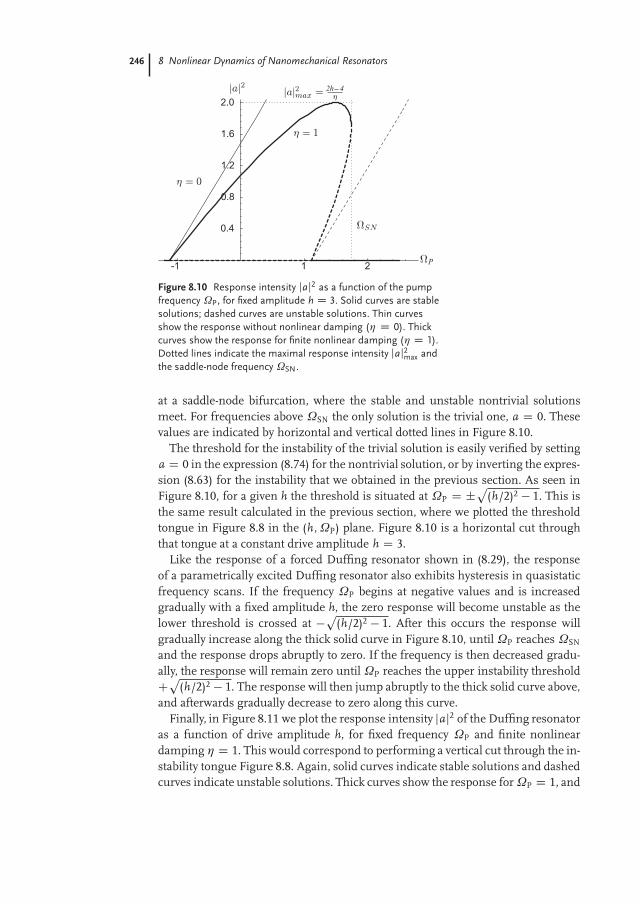
Finally, in Figure 8.11 we plot the response intensity jaj2 of the Duffing resonatoras a function of drive amplitude h, for fixed frequency ΩP and finite nonlineardamping η D 1. This would correspond to performing a vertical cut through the in-stability tongue Figure 8.8. Again, solid curves indicate stable solutions and dashedcurves indicate unstable solutions. Thick curves show the response for ΩP D 1, and
8.3 Parametric Excitation of a Damped Duffing Resonator 247
1 2 3 4
0.8
1.6
2.4
3.2
4.0
P
P
P
Figure 8.11 Response intensity jaj2 as a function of the para-metric drive amplitude h for fixed frequency ΩP and finite non-linear damping (η D 1). Thick curves show the stable (solidcurves) and unstable (dashed curves) response for ΩP D 1.Thin curves show the stable solutions for ΩP D η/3 andΩP D 1, and demonstrate that hysteresis as h is varied isexpected only for ΩP > η/3.
thin curves show the response for ΩP D η/3 and ΩP D 1. The intersection ofthe trivial and the nontrivial solutions, which corresponds to the instability thresh-old (8.63), occurs at h D 2
pΩP
2 C 1. For ΩP < η/3, the nontrivial solution forjaj2 grows continuously for h above threshold and is stable. This is a supercriticalbifurcation. On the other hand, for ΩP > η/3 the bifurcation is subcritical and thenontrivial solution grows for h below threshold. This solution is unstable until thecurve of jaj2 as a function of h turns at a saddle-node bifurcation at
hSN D 2 C 2η3 ΩPq
1 C η3
2, (8.77)
where the solution becomes stable and jaj2 is once more an increasing functionof h. For amplitudes h < hSN the only solution is the trivial one a D 0. Hystereticbehavior is therefore expected for quasistatic scans of the drive amplitude h only ifthe fixed frequency ΩP > η/3, as can be inferred from Figure 8.11.
8.3.5Parametric Excitation at the Second Instability Tongue
We wish to examine the second tongue by looking at the response above thresholdand highlighting the main changes from the first tongue. This tongue, it shouldbe noted, is readily accessible in experiments because the pump and the responsefrequencies are the same. We start with the general equation for a parametrically-driven Duffing resonator (8.44), but with no direct drive (g D 0), where the para-metric excitation is performed around 1 instead of 2. Correspondingly, the scalingof H with respect to needs to be changed to H D h
p. The reason for this change
248 8 Nonlinear Dynamics of Nanomechanical Resonators
is that with the H D h scaling, the order 1/2 term in x becomes identically zero.This occurs because the parametric driving term does not contribute to the order3/2 secular term which we use to find the response. Scaling H in the appropriatemanner will introduce a nonsecular correction to x at order , and this correctionwill contribute to the order 3/2 secular term and will give us the required response.The equation of motion then becomes
Rx C x D h1/2
2
ei(tCΩPT ) C c.c.
x Px x3 ηx2 Px , (8.78)
and we try an expansion of the solution of the form
x (t) D 1/2 12
A(T ) eit C c.c.
C x1/2(t) C 3/2x1(t) C . . . (8.79)
Substituting this expansion into the equation of motion (8.78), we obtain at order1/2 the linear equation as usual, and at order
Rx1/2 C x1/2 D h
4
A eiΩPT e2it C A eiΩP T C c.c.
. (8.80)
As expected, there is no secular term on the right-hand side so we can immediatelysolve for x1/2, yielding
x1/2(t) D h
4
A
3eiΩP T e2 it A eiΩP T C c.c.
C O() . (8.81)
Substituting the solution for x1/2 into the expansion (8.79), and the expansion backinto the equation of motion (8.78), contributes an additional term from the para-metric driving which has the form
3/2 h2
8
A
3eiΩP T e2 it C A eiΩP T C c.c.
eiΩP T eit C c.c.
D 3/2 h2
8
23
A C A ei2ΩP T
eit C c.c. C nonsecular terms . (8.82)
This gives us the required contribution to the equation for the vanishing secularterms. All other terms remain as they were in (8.47), so that the new equation fordetermining A(T ) becomes
dA
dTC i
h2
8
23
A C A ei2ΩP T
C 1
2A i
38
jAj2A C η8
jAj2A D 0 . (8.83)
Again, ignoring initial transients and assuming that the nonlinear terms in theequation are sufficient to saturate the growth of the instability, we try a steady-statesolution, this time of the form
A(T ) D a eiΩP T . (8.84)
The solution to the equation of motion (8.78) is therefore
x (t) D 1/2(a ei(1CΩP)t C c.c.) C O() , (8.85)

8.3 Parametric Excitation of a Damped Duffing Resonator 249
where the correction x1/2 of order is given in (8.81) and, as before, we are notinterested in the correction x1(t) of order 3/2, but rather in the fixed amplitudea of the lowest order term. We substitute the steady-state solution (8.84) into theequation of the secular terms (8.83) and obtain
34
jaj2 2ΩP h2
6
C i
1 C η
4jaj2
a D h2
4a . (8.86)
By taking the magnitude squared of both sides we obtain, in addition to the trivialsolution a D 0, a nontrivial response given by
34
jaj2 2ΩP 16
h22
C
1 C η4
jaj22 D h4
16. (8.87)
Figure 8.12 shows the response intensity jaj2 as a function of the frequency ΩP
for a fixed drive amplitude of h D 3, producing a horizontal cut through the sec-ond instability tongue. The solution looks very similar to the response shown inFigure 8.10 for the first instability tongue, though we should point out two im-portant differences. The first is that the orientation of the ellipse, indicated by theslope of the curves for η D 0, is different. The slope here is 8/3, whereas for thefirst instability tongue the slope is 4/3. The second is the change in the scaling ofh with , or the inverse quality factor Q1. The lowest critical drive amplitude foran instability at the second tongue is again on resonance (ΩP D 0), and its value isagain h D 2. This now implies, however, that H
pQ D 2, or that H scales as the
square root of the linear damping rate Γ . This is consistent with the well knownresult that the minimal amplitude for the instability of the nth tongue scales asΓ 1/n (for example, see [42], Section 3).
-2 -1 1 2
0.8
1.6
2.4
3.2
4.0
4.8
P
Figure 8.12 Response intensity jaj2 of a parametrically-drivenDuffing resonator as a function of the pump frequency ΩP, fora fixed amplitude h D 3 in the second instability tongue. Solidcurves are stable solutions and dashed curves are unstablesolutions. Thin curves show the response without nonlineardamping (η D 0). Thick curves show the response for finitenonlinear damping (η D 1).
250 8 Nonlinear Dynamics of Nanomechanical Resonators
8.4Parametric Excitation of Arrays of Coupled Duffing Resonators
The last two sections of this review describe theoretical work that was motivateddirectly by the experimental work of Buks and Roukes [8]. They fabricated an ar-ray of nonlinear micromechanical doubly-clamped gold beams, and excited themparametrically by modulating the strength of an externally controlled electrostat-ic coupling between neighboring beams. The Buks and Roukes experiment wasmodeled by Lifshitz and Cross [44] (henceforth LC) using a set of coupled nonlin-ear equations of motion. The latter used secular perturbation theory, as we havedescribed so far for a system with just a single degree of freedom, to convert theseequations of motion into a set of coupled nonlinear algebraic equations for the nor-mal mode amplitudes of the system. This enabled them to obtain exact results forsmall arrays, but only a qualitative understanding of the dynamics of large arrays.We shall review these results in this section.
In order to obtain analytical results for large arrays, Bromberg, Cross, and Lif-shitz [7] (henceforth BCL) studied the same system of equations, approaching itfrom the continuous limit of infinitely many degrees of freedom. They obtaineda description of the slow spatiotemporal dynamics of the array of resonators interms of an amplitude equation. BCL showed that this amplitude equation couldpredict the initial mode that develops at the onset of parametric oscillations as thedriving amplitude is gradually increased from zero, as well as a sequence of sub-sequent transitions to other single mode oscillations. We shall review these resultsin Section 8.5. Kenig, Lifshitz, and Cross [38] have extended the investigation ofthe amplitude equation to more general questions such as how patterns are se-lected when many patterns or solutions are simultaneously stable. This extensionincludes other experimentally relevant questions, such as the response of the sys-tem of coupled resonators to time dependent sweeps of the control parameters,rather than quasistatic sweeps like the ones we have been discussing here. Keniget al. [39] have also studied the formation and dynamics of intrinsically-localizedmodes, or solitons, in the array equations of LC. To this end, they derived a differ-ent amplitude equation, which takes the form of a parametrically-driven dampednonlinear Shrödinger equation, also known as a forced complex Ginzburg-Landauequation. We shall not review these last two papers here, but encourage the readerto pursue them independently.
8.4.1Modeling an Array of Coupled Duffing Resonators
LC modeled the array of coupled nonlinear resonators that was studied by Buksand Roukes using a set of coupled equations of motion (EOM) of the form
Ru n C u n C u3n 1
2 Q1( Pu nC1 2 Pu n C Pu n1)
C 12
D C H cos ωp t
(u nC1 2u n C u n1)
12 η
(u nC1 u n)2( Pu nC1 Pu n) (u n u n1)2( Pu n Pu n1)
D 0 ,
(8.88)
8.4 Parametric Excitation of Arrays of Coupled Duffing Resonators 251
where u n(t) describes the deviation of the nth resonator from its equilibrium, withn D 1 . . . N , and fixed boundary conditions u0 D u NC1 D 0. Detailed argu-ments for the choice of terms introduced into the equations of motion are dis-cussed in [44]. The terms include an elastic restoring force with both linear andcubic contributions, whose coefficients are both scaled to 1 as in our discussion ofthe single degree of freedom. They also include a dc electrostatic nearest neighborcoupling term with a small ac component responsible for the parametric excita-tion, with coefficients D and H, respectively, and linear as well as cubic nonlineardissipation terms. Both dissipation terms are assumed to depend on the differenceof the displacements of nearest neighbors.
We consider here a slightly simpler and more general model for an array ofcoupled resonators in order to illustrate the approach. Motivated by the geome-try of most experimental NEMS systems, we assume a line of identical resonatorsalthough the generalization to two or three dimensions is straightforward. Thesimplest model is to take the equation of motion of each resonator to be as thatin (8.44), with the addition of a coupling term to its two neighbors. A simple choicewould be to assume that this coupling does not introduce additional dissipation,which we describe as reactive coupling. Elastic and electrostatic coupling might bepredominantly of this type. After the usual scaling, the equations of motions wouldtake the form
Ru n C Q1 Pu n C u3n C (1 C H cos ωP t)u n C ηu2
n Pu n
C 12 D(u nC1 2u n C u n1) D 0 , (8.89)
where we do not take into account any direct drive for the purposes of the presentsection.
The equations of motion for particular experimental implementations mighthave different terms, although we expect all will have linear and nonlinear damp-ing, linear coupling, and parametric drive. For example, to model the experimentalsetup of Buks and Roukes [8], LC supposed that both linear and nonlinear dissipa-tion terms involved the difference of neighboring displacements, that is, the termsinvolving Pu n in our equations of motion (8.89) are replaced with terms involvingu nC1 u n in the equations of motion (8.88) used by LC. This was to describe thephysics of electric current damping, with the currents driven by the varying ca-pacitance between neighboring resonators depending on the change in separationand the fixed DC voltage. This effect seemed to be the dominant component of thedissipation in the Buks and Roukes experiments. Similarly, the parametric driveH cos ωP t multiplied (u nC1 2u n C u n1) in the equations of LC rather than u n
here, since the voltage between adjacent resonators was the quantity modulated,changing the electrostatic component of the spring constant.
In a more recent implementation [45], the electric current damping has beenreduced, and the parametric drive is directly applied to each resonator piezoelectri-cally, so that the simpler form of (8.89) applies. The method of attack is the samein any case. We will illustrate the approach on the simpler equation, and referthe reader to LC for the more complicated model. An additional complication ina realistic model may be that the coupling is longer range than nearest neighbor.
252 8 Nonlinear Dynamics of Nanomechanical Resonators
For example, both electrostatic coupling and elastic coupling through the supportswould have longer range components. The general method is the same for theseadditional effects, and the reader should be able to apply the approach to the modelfor their particular experimental implementation.
8.4.2Calculating the Response of an Array
We calculate the response of the array to parametric excitation, again using secularperturbation theory. We suppose Q is large and take D Q1 as the small expan-sion parameter. As in Section 8.3 we take H D h, but we also take D D d sothat the width of the frequency band of eigenmodes is also small. This is not quitehow LC treated the coupling, but we think the present approach is clearer, and itis equivalent up to the order of the expansion in that we require. We thank EyalKenig for pointing out this simplification.
The equations of motion are now
Ru n C Pu n C u3n C
1 C h cos(2 C ΩP)t
u n C ηu2
n Pu n
C 12 d(u nC1 2u n C u n1) D 0 , n D 1 . . . N . (8.90)
We expand u n(t) as a sum of standing wave modes with slowly varying amplitudes.The nature of the standing wave modes will depend on the conditions at the end ofthe line of resonators. In the experiments of Buks and Roukes there were N mobilebeams, with a number of identical immobilized beams at each end. These condi-tions can be implemented in a nearest neighbor model by taking two additionalresonators, u0 and u NC1 and assuming
u0 D u NC1 D 0 . (8.91)
The standing wave modes are then
u n D sin(nqm) with qm D mπN C 1
, m D 1 . . . N . (8.92)
On the other hand, for a line of N resonators with free ends there is no force fromoutside the line. For the nearest neighbor model this can be imposed again bytaking two additional resonators, but now with the conditions
u0 D u1 and u N D u NC1 . (8.93)
The standing wave modes are now
u n D cos
n 12
qm
with qm D mπ
N, m D 0 . . . N 1 . (8.94)
For our illustration we will take (8.91), (8.92). Thus we write
u n(t) D 1/2 12
NXmD1
A m(T ) sin(nqm) eit C c.c.
C 3/2u(1)n (t) C . . . ,
n D 1 . . . N , (8.95)
with qm as in (8.92).
8.4 Parametric Excitation of Arrays of Coupled Duffing Resonators 253
We substitute the trial solution (8.95) into the EOM term by term. Up to order3/2 we have
Ru n D 1/2 12
Xm
sin(nqm)A m C 2 iA0
m
eit C c.c.
C 3/2 Ru(1)n (t) C . . . ,
(8.96a)
Pu n D 3/2 12
Xm
sin(nqm)iA m eit C c.c.
C . . . , (8.96b)
12
d(u nC1 2u n C u n1)
D 3/2 d
2
Xm
2 sin2 qm
2
sin(nqm)
A m eit C c.c.
C . . . (8.96c)
u3n D 3/2 1
8
Xj,k ,l
sin(nq j ) sin(nqk) sin(nql)
A j eit C c.c.
A k eit C c.c.
A l eit C c.c.
D 3/2 1
32
Xj,k ,l
˚sin[n(q j C qk C q l)] C sin[n(q j qk C q l )]
C sinn(q j C qk q l)
sinn(q j C qk C q l)
˚
A j A k A l e3 it C 3A j A k Al eit C c.c.
, (8.96d)
and
ηu n2 Pu n D 3/2 η
32
Xj,k ,l
˚sin[n(q j C qk C q l)] C sin[n(q j qk C q l)]
C sin[n(q j C qk q l)] sin[n(q j C qk C q l)]
A j eit C c.c.
A k eit C c.c.
iA l eit C c.c.
.
(8.96e)
The order 1/2 terms cancel, and at order 3/2 we get N equations of the form
Ru(1)n C u
(1)n D
Xm
(mth secular term) eit C other terms , (8.97)
where the left-hand sides are uncoupled linear harmonic oscillators, with a fre-quency unity. On the right-hand sides we have N secular terms which act to drivethe oscillators u
(1)n at their resonance frequencies. As we did for all the single res-
onator examples, here, too, we require that all the secular terms vanish so thatthe u
(1)n remain finite. Thus, we obtain equations for the slowly varying amplitudes
A m(T ). To extract the equation for the mth amplitude A m(T ) we make use of theorthogonality of the modes, multiplying all the terms by sin(nqm) and summingover n. We find that the coefficient of the mth secular term, which is required to
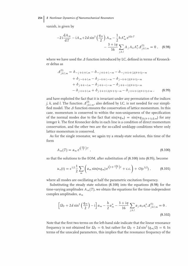
254 8 Nonlinear Dynamics of Nanomechanical Resonators
vanish, is given by
2 idA m
dT iA mC2d sin2
qm
2
A m 1
2hA
m eiΩP T
3 C iη16
Xj,k ,l
A j A k Al ∆(1)
j k lIm D 0 , (8.98)
where we have used the ∆ function introduced by LC, defined in terms of Kroneck-er deltas as
∆(1)j k lIm
D δ j CkCl,m δ j CkCl,m δ j CkCl,2(NC1)m
C δ j kCl,m δ j kCl,m δ j kCl,2(NC1)m
C δ j Ckl,m δ j Ckl,m δ j Ckl,2(NC1)m
δ j CkCl,m C δ j CkCl,2(NC1)m δ j CkCl,2(NC1)Cm , (8.99)
and have exploited the fact that it is invariant under any permutation of the indicesj, k, and l. The function ∆(2)
j k lIm, also defined by LC, is not needed for our simpli-
fied model. The ∆ function ensures the conservation of lattice momentum. In thiscase, momentum is conserved to within the non-uniqueness of the specificationof the normal modes due to the fact that sin(nqm) D sin(nq2k(NC1)˙m) for anyinteger k. The first Kronecker delta in each line is a condition of direct momentumconservation, and the other two are the so-called umklapp conditions where onlylattice momentum is conserved.
As for the single resonator, we again try a steady-state solution, this time of theform
A m(T ) D am ei
ΩP2
T , (8.100)
so that the solutions to the EOM, after substitution of (8.100) into (8.95), become
u n(t) D 1/2 12
Xm
am sin(nqm) ei
1C
ΩP2
t C c.c.
C O(3/2) , (8.101)
where all modes are oscillating at half the parametric excitation frequency.Substituting the steady state solution (8.100) into the equations (8.98) for the
time-varying amplitudes A m(T ), we obtain the equations for the time-independentcomplex amplitudes, am
hΩP C 2d sin2
qm
2
i
iam h
2a
m 3 C iη16
Xj,k ,l
a j ak al ∆(1)
j k lImD 0 .
(8.102)
Note that the first two terms on the left-hand side indicate that the linear resonancefrequency is not obtained for ΩP D 0, but rather for ΩP C 2d sin2 (qm/2) D 0. Interms of the unscaled parameters, this implies that the resonance frequency of the
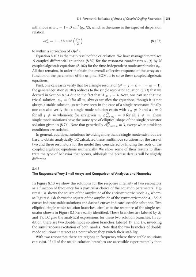
8.4 Parametric Excitation of Arrays of Coupled Duffing Resonators 255
mth mode is ωm D 1 D sin2 (qm/2), which is the same as the expected dispersionrelation
ω2m D 1 2D sin2
qm
2
(8.103)
to within a correction of O(2).Equation 8.102 is the main result of the calculation. We have managed to replace
N coupled differential equations (8.89) for the resonator coordinates u n(t) by N
coupled algebraic equations (8.102) for the time-independent mode amplitudes am .All that remains, in order to obtain the overall collective response of the array as afunction of the parameters of the original EOM, is to solve these coupled algebraicequations.
First, one can easily verify that for a single resonator (N D j D k D l D m D 1),the general equation (8.102) reduces to the single resonator equation (8.73) that wederived in Section 8.3.4 due to the fact that ∆111I1 D 4. Next, one can see that thetrivial solution, am D 0 for all m, always satisfies the equations, though it is notalways a stable solution, as we have seen in the case of a single resonator. Finally,one can also verify that a single mode solution exists with am ¤ 0 and a j D 0for all j ¤ m whenever, for any given m, ∆(1)
mmmI j D 0 for all j ¤ m. Thesesingle mode solutions have the same type of elliptical shape of the single resonatorsolution given in (8.74). Note that generically ∆(1)
mmmIm D 3, except when umklappconditions are satisfied.
In general, additional solutions involving more than a single mode exist, but arehard to obtain analytically. LC calculated these multimode solutions for the case oftwo and three resonators for the model they considered by finding the roots of thecoupled algebraic equations numerically. We show some of their results to illus-trate the type of behavior that occurs, although the precise details will be slightlydifferent.
8.4.3The Response of Very Small Arrays and Comparison of Analytics and Numerics
In Figure 8.13 we show the solutions for the response intensity of two resonatorsas a function of frequency for a particular choice of the equation parameters. Fig-ure 8.13a shows the square of the amplitude of the antisymmetric mode a2, where-as Figure 8.13b shows the square of the amplitude of the symmetric mode a1. Solidcurves indicate stable solutions and dashed curves indicate unstable solutions. Twoelliptical single mode solution branches, similar to the response of the single res-onator shown in Figure 8.10 are easily identified. These branches are labeled by S1
and S2. LC give the analytical expressions for these two solution branches. In ad-dition, there are two double mode solution branches, labeled D1 and D2, involvingthe simultaneous excitation of both modes. Note that the two branches of doublemode solutions intersect at a point where they switch their stability.
With two resonators there are regions in frequency where three stable solutionscan exist. If all of the stable solution branches are accessible experimentally then
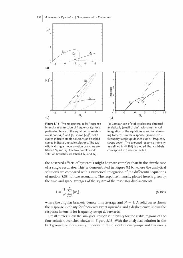
256 8 Nonlinear Dynamics of Nanomechanical Resonators
0
1|2
Ω
Ω-2 2 4 6
0-2 2 4 6
D1
D1
D2
D2
S1
S2
2|2
0
1
2
0
1
2
0
1
2
3
4
5
-1 0 -5 0 5 1 0Ω
Res
po
nse
S2
S1
D1
D2
(a)
(b) (c)
P
P P
Figure 8.13 Two resonators. (a,b) Responseintensity as a function of frequency ΩP for aparticular choice of the equation parameters.(a) shows ja2j2 and (b) shows ja1j2. Solidcurves indicate stable solutions and dashedcurves indicate unstable solutions. The twoelliptical single mode solution branches arelabeled S1 and S2. The two double modesolution branches are labeled D1 and D2.
(c) Comparison of stable solutions obtainedanalytically (small circles), with a numericalintegration of the equations of motion show-ing hysteresis in the response (solid curve –frequency swept up; dashed curve – frequencyswept down). The averaged response intensityas defined in (8.104) is plotted. Branch labelscorrespond to those on the left.
the observed effects of hysteresis might be more complex than in the simple caseof a single resonator. This is demonstrated in Figure 8.13c, where the analyticalsolutions are compared with a numerical integration of the differential equationsof motion (8.88) for two resonators. The response intensity plotted here is given bythe time and space averages of the square of the resonator displacements
I D 1N
NXnD1
˝u2
n
˛, (8.104)
where the angular brackets denote time average and N D 2. A solid curve showsthe response intensity for frequency swept upwards, and a dashed curve shows theresponse intensity for frequency swept downwards.
Small circles show the analytical response intensity for the stable regions of thefour solution branches shown in Figure 8.13. With the analytical solution in thebackground, one can easily understand the discontinuous jumps and hysteresis
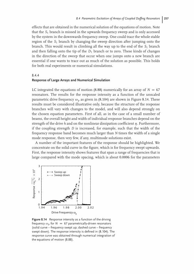
8.4 Parametric Excitation of Arrays of Coupled Duffing Resonators 257
effects that are obtained in the numerical solution of the equations of motion. Notethat the S1 branch is missed in the upwards frequency sweep and is only accessedby the system in the downwards frequency sweep. One could trace the whole stableregion of the S1 branch by changing the sweep direction after jumping onto thebranch. This would result in climbing all the way up to the end of the S1 branchand then falling onto the tip of the D1 branch or to zero. These kinds of changesin the direction of the sweep that occur when one jumps onto a new branch areessential if one wants to trace out as much of the solution as possible. This holdsfor both real experiments or numerical simulations.
8.4.4Response of Large Arrays and Numerical Simulation
LC integrated the equations of motion (8.88) numerically for an array of N D 67resonators. The results for the response intensity as a function of the unscaledparametric drive frequency ωp as given in (8.104) are shown in Figure 8.14. Theseresults must be considered illustrative only, because the structure of the responsebranches will vary with changes to the model, and will also depend strongly onthe chosen equation parameters. First of all, as in the case of a small number ofbeams, the overall height and width of individual response branches depend on thestrength of the drive h and on the nonlinear dissipation coefficient η. Furthermore,if the coupling strength D is increased, for example, such that the width of thefrequency response band becomes much larger than N times the width of a singlemode response, then very few, if any, multimode solutions exist.
A number of the important features of the response should be highlighted. Weconcentrate on the solid curve in the figure, which is for frequency swept upwards.First, the response intensity shows features that span a range of frequencies that islarge compared with the mode spacing, which is about 0.0006 for the parameters
0
1
2
3
1.9 4 1.9 6 1.9 8 2.0 0 2.0 2
Drive Frequenzy ωp
Sweep upSweep down
Res
po
nse
<u n
2>
× 10
3
Figure 8.14 Response intensity as a function of the drivingfrequency ωp for N D 67 parametrically-driven resonators(solid curve – frequency swept up; dashed curve – frequencyswept down). The response intensity is defined in (8.104). Theresponse curve was obtained through numerical integration ofthe equations of motion (8.88).
258 8 Nonlinear Dynamics of Nanomechanical Resonators
used. The reason for this is that we skip over many others as we follow a particularsolution, as has been seen for the S1 branch in the two resonator case. Second,the variation of the response with frequency shows abrupt jumps as the frequencyis raised, particularly on the high frequency side of the features. This happens aswe reach saddle-node or other types of bifurcations where we lose the stability ofthe solution branch, or the branch ends altogether. Third, the response extends tofrequencies higher than the band edge for the linear modes, which would give aresponse only up to ωp D 2.0. This happens simply due to the positive Duffingparameter which causes frequency pulling to the right. Note that the downwardssweep is able to access additional stable solution branches that were missed in theupwards sweep. There is also no response above ωp D 2.0 in this case. This is be-cause the zero displacement state is stable for ωp > 2.0, and the system will remainin this state as the frequency is lowered unless a large enough disturbance kicks itonto another of the solution branches. The hysteresis on reversing the frequencysweep was not examined in any experiment, and it would be interesting to test thisprediction of LC in the future.
8.5Amplitude Equation Description for Large Arrays
We finish this review by describing the approach used by BCL [6, 7] to obtain an-alytical results for large arrays by approaching them from the continuous limit ofinfinitely many degrees of freedom. We only summarize the main results of BCLand encourage the reader, who by now has all the required background, to referto BCL [7] and to Kenig et al. [38] for details of the derivation and for thoroughdiscussions of the results and their experimental consequences. We note that BCLstudied the original system of (8.88), where both the parametric excitation and thedamping are introduced in terms of the difference variables u nC1 u n . We stickto this model here, and leave it to the reader as an exercise to generalize the BCLderivation for the more general model equations (8.89) that we used in the previoussection.
A novel feature of the parametrically-driven instability is that the bifurcation tostanding waves switches from supercritical (continuous) to subcritical (discontinu-ous) at a wave number at or close to the critical one, for which the required para-metric driving force is minimum. This changes the form of the amplitude equationthat describes the onset of the parametrically-driven waves so that it no longer hasthe standard “Ginzburg–Landau” form [20]. The central result of BCL is this newscaled amplitude equation (8.112), which is governed by a single control parame-ter and captures the slow dynamics of the coupled resonators just above the onsetof parametric oscillations, including this unusual bifurcation behavior. BCL con-firmed the behavior numerically and made suggestions for testing it experimen-tally. Kenig et al. [38] have extended the investigation of the amplitude equationto include such situations as time-dependent ramps of the drive amplitude, as op-posed to the standard quasistatic sweeps of the control parameters. Although our
8.5 Amplitude Equation Description for Large Arrays 259
focus here is on parametrically-driven NEMS & MEMS resonators, we should em-phasize that the amplitude equation of BCL that we describe here should also applyto other parametrically-driven wave systems with weak nonlinear damping.
8.5.1Amplitude Equations for Counter Propagating Waves
BCL scaled the equations of motion (8.88), as did Lifshitz and Cross [44], withoutassuming a priori that the coupling D is small. Thus, the scaled equations of mo-tion that they solved were
Ru n C u n C u3n 1
2 ( Pu nC1 2 Pu n C Pu n1)
C 12
D C h cos(2ω p t)
(u nC1 2u n C u n1)
12 η
(u nC1 u n)2( Pu nC1 Pu n) (u n u n1)2( Pu n Pu n1)
D 0 .
(8.105)
Note the way in which the pump frequency is specified as 2ωp in the argument ofthe cosine term, with an explicit factor of two (unlike what we did in Section 8.4),and also without making any assumptions at this point regarding its deviation fromtwice the resonance. We also remind the reader that this and all other frequenciesare measured in terms of the natural frequency of a single resonator, which hasbeen scaled to 1. The first step in treating this system of equations analytically is tointroduce a continuous displacement field u(x , t), and slow spatial and temporalscales X D x and T D t. One then tries a solution in terms of a pair of counter-propagating plane waves at half the pump frequency, which is a natural first guessin continuous parametrically-driven systems such as Faraday waves [20]. This yields
u(x , t) D 1/2 AC(X , T ) eiqp x C A
(X , T ) eiqp x
eiωp t C c.c.
C 3/2u(1)(x , t, X , T ) C . . . , (8.106)
where qp and ωp are related through the dispersion relation (8.103)
ω2p D 1 2D sin2
qp
2
. (8.107)
By substituting this ansatz (8.106) into the equations of motion (8.105) and ap-plying a solvability condition on the terms of order 3/2, BCL obtained a pair ofcoupled amplitude equations for the counterpropagating wave amplitudes A˙
@A˙
@T˙ vg
@A˙
@XD sin2
qp
2
A˙ i
h
2ω p
sin2 qp
2
A
4η sin4 qp
2
i
32ωp
jA˙j2 C 2jAj2A˙ , (8.108)
where the upper signs (lower signs) give the equation for AC (A) and
vg D @ωp
@qpD D sin(qp)
2ωp(8.109)
260 8 Nonlinear Dynamics of Nanomechanical Resonators
is the group velocity. This equation is the extension of (8.47) to many coupled res-onators, only now the parametric drive couples amplitudes of the two counterprop-agating waves AC and A instead of coupling A and A. A detailed derivation ofthe amplitude equations (8.108) can be found in [6, 7]. We should note that similarequations were previously derived for describing Faraday waves [29, 46].
By linearizing the amplitude equations (8.108) about the zero solution (AC DA D 0), we find that the linear combination of the two amplitudes that firstbecomes unstable at h D hc 2ωp is B / (AC iA). This represents theemergence of a standing wave with a temporal phase of π/4 relative to the drive.However, the orthogonal linear combination of the amplitudes decays exponential-ly and does not participate in the dynamics at onset. Thus, just above threshold asingle amplitude equation should suffice, describing this standing wave pattern.We describe the derivation of this equation in the next section.
8.5.2Reduction to a Single Amplitude Equation
Nonlinear dissipation plays an important role in the saturation of the responseto parametric excitation, as we saw in Section 8.3.4. Thus, it is natural to try tokeep a balance between the strength of this nonlinearity and the amount by whichwe drive the system above threshold. Assuming that the nonlinear damping isweak, we use it to define a second small parameter δ D p
η. This particulardefinition turns out to be useful if we then scale the reduced driving amplitude(h hc)/ hc linearly with δ, defining a scaled reduced driving amplitude r by let-ting (h hc)/ hc r δ. We can then treat the initial linear combination of the twoamplitudes in (8.108) that becomes unstable by introducing a second ansatz,
AC
A
D δ1/4
1i
B( , τ) C δ3/4
w (1)(X , T, , τ)v (1)(X , T, , τ)
C δ5/4
w (2)(X , T, , τ)v (2)(X , T, , τ)
, (8.110)
where D δ1/2 X and τ D δT . Substitution of this ansatz allows one to obtain thecorrection to the solution at order δ3/4
w (1)
v (1)
D 1
2 sin2(q p /2)
vg
@B
@C i
92ω p
jBj2B
1i
, (8.111)
after which a solvability condition applied to the terms of order δ5/4 yields an equa-tion for the field B( , τ). After scaling, this takes the form
@B
@τD r B C @2 B
@ 2C i
23
4jBj2 @B
@C B2 @B
@
2jBj2B jBj4B . (8.112)
This is the BCL amplitude equation. It is governed by a single control parameter,the reduced drive amplitude r, and captures the slow dynamics of the coupled res-onators just above the onset of parametric oscillations. The reader is encouraged
8.5 Amplitude Equation Description for Large Arrays 261
to consult [7] for a more detailed account of the derivation of the BCL equation.The form of (8.112) is also applicable to the onset of parametrically driven standingwaves in continuum systems with weak nonlinear damping, and combines in asingle equation a number of effects studied previously [13, 14, 23, 29, 46, 53].
8.5.3Single Mode Oscillations
Now that this novel amplitude equation has been derived by BCL it can be used tostudy a variety of dynamical solutions, ranging from simple single mode to morecomplicated nonlinear extended solutions and, after slight modifications, also forthe dynamics of localized solutions. BCL used the amplitude equation to study thestability of single mode steady-state solutions
B D bk eik , (8.113)
that is, standing wave solutions that consist of a single sine wave pattern with oneof the allowed wave vectors qm . The wave vector k gives, in some scaled units, thedifference between the wave vector qp determined by the pump frequency throughthe dispersion relation, and the wave vector qm D mπ/(N C 1), m D 1 . . . N , of theactual mode that is selected by the system.
A number of interesting results are readily evident if we simply substitute thesingle mode solution (8.113) into the BCL amplitude equation (8.112). From thelinear terms in the amplitude equation we find, as expected, that for r > k2 thezero displacement solution is unstable to small perturbations of the form of (8.113).This defines the parabolic neutral stability curve, which is shown as a dashed linein Figure 8.15. The nonlinear gradients and the cubic term take the simple form2(k 1)jbk j2bk . For k < 1 these terms immediately act to saturate the growthof the amplitude assisted by the quintic term. Standing waves therefore bifurcatesupercritically from the zero displacement state. For k > 1 the cubic terms act toincrease the growth of the amplitude, and saturation is achieved only by the quinticterm. Standing waves therefore bifurcate subcritically from the zero displacementstate. The saturated amplitude jbk j, obtained by setting (8.112) to zero, is given by
jbk j2 D (k 1) ˙q
(k 1)2 C (r k2) 0 . (8.114)
In Figure 8.16 we plot jbk j2 as a function of the reduced driving amplitude r forthree different wave number shifts k. The solid (dashed) lines are the stable (un-stable) solutions of (8.114). The circles were obtained by numerical integration ofthe equations of motion (8.105). For each driving amplitude, the Fourier compo-nents of the steady state solution were computed to verify that only single modesare found, suggesting that in this regime of parameters only these states are stable.
BCL showed the power of the amplitude equation in predicting the first singlemode solution that should appear at onset. In addition it also predicts the sequenceof Eckhaus instabilities that switch to other single mode solutions as the reduced
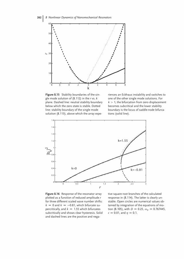
262 8 Nonlinear Dynamics of Nanomechanical Resonators
8 6 4 2 0 2 4 60
10
20
30
40
50
60
k
Figure 8.15 Stability boundaries of the sin-gle mode solution of (8.112) in the r vs. kplane. Dashed line: neutral stability boundarybelow which the zero state is stable. Dottedline: stability boundary of the single modesolution (8.113), above which the array expe-
riences an Eckhaus instability and switches toone of the other single mode solutions. Fork > 1, the bifurcation from zero displacementbecomes subcritical and the lower stabilityboundary is the locus of saddle-node bifurca-tions (solid line).
0 0.5 1 1.5 2 2.50
0.2
0.4
0.6
0.8
1
1.2
1.4
1.6
1.8
r
k=1.55
k=–0.81k=0
Figure 8.16 Response of the resonator arrayplotted as a function of reduced amplitude rfor three different scaled wave number shifts:k D 0 and k D 0.81, which bifurcate su-percritically, and k D 1.55 which bifurcatessubcritically and shows clear hysteresis. Solidand dashed lines are the positive and nega-
tive square root branches of the calculatedresponse in (8.114). The latter is clearly un-stable. Open circles are numerical values ob-tained by integration of the equations of mo-tion (8.105), with D D 0.25, ωp D 0.767445, D 0.01, and η D 0.1.
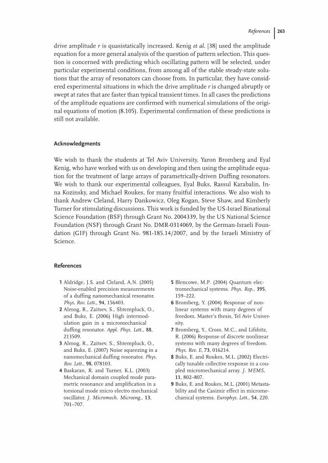
References 263
drive amplitude r is quasistatically increased. Kenig et al. [38] used the amplitudeequation for a more general analysis of the question of pattern selection. This ques-tion is concerned with predicting which oscillating pattern will be selected, underparticular experimental conditions, from among all of the stable steady-state solu-tions that the array of resonators can choose from. In particular, they have consid-ered experimental situations in which the drive amplitude r is changed abruptly orswept at rates that are faster than typical transient times. In all cases the predictionsof the amplitude equations are confirmed with numerical simulations of the origi-nal equations of motion (8.105). Experimental confirmation of these predictions isstill not available.
Acknowledgments
We wish to thank the students at Tel Aviv University, Yaron Bromberg and EyalKenig, who have worked with us on developing and then using the amplitude equa-tion for the treatment of large arrays of parametrically-driven Duffing resonators.We wish to thank our experimental colleagues, Eyal Buks, Rassul Karabalin, In-na Kozinsky, and Michael Roukes, for many fruitful interactions. We also wish tothank Andrew Cleland, Harry Dankowicz, Oleg Kogan, Steve Shaw, and KimberlyTurner for stimulating discussions. This work is funded by the US-Israel BinationalScience Foundation (BSF) through Grant No. 2004339, by the US National ScienceFoundation (NSF) through Grant No. DMR-0314069, by the German-Israeli Foun-dation (GIF) through Grant No. 981-185.14/2007, and by the Israeli Ministry ofScience.
References
1 Aldridge, J.S. and Cleland, A.N. (2005)Noise-enabled precision measurementsof a duffing nanomechanical resonator.Phys. Rev. Lett., 94, 156403.
2 Almog, R., Zaitsev, S., Shtempluck, O.,and Buks, E. (2006) High intermod-ulation gain in a micromechanicalduffing resonator. Appl. Phys. Lett., 88,213509.
3 Almog, R., Zaitsev, S., Shtempluck, O.,and Buks, E. (2007) Noise squeezing in ananomechanical duffing resonator. Phys.
Rev. Lett., 98, 078103.4 Baskaran, R. and Turner, K.L. (2003)
Mechanical domain coupled mode para-metric resonance and amplification in atorsional mode micro electro mechanicaloscillator. J. Micromech. Microeng., 13,701–707.
5 Blencowe, M.P. (2004) Quantum elec-tromechanical systems. Phys. Rep., 395,159–222.
6 Bromberg, Y. (2004) Response of non-linear systems with many degrees offreedom. Master’s thesis, Tel Aviv Univer-sity.
7 Bromberg, Y., Cross, M.C., and Lifshitz,R. (2006) Response of discrete nonlinearsystems with many degrees of freedom.Phys. Rev. E, 73, 016214.
8 Buks, E. and Roukes, M.L. (2002) Electri-cally tunable collective response in a cou-pled micromechanical array. J. MEMS,11, 802–807.
9 Buks, E. and Roukes, M.L. (2001) Metasta-bility and the Casimir effect in microme-chanical systems. Europhys. Lett., 54, 220.
264 References
10 Buks, E. and Yurke, B. (2006) Mass de-tection with a nonlinear nanomechanicalresonator. Phys. Rev. E, 74, 046619.
11 Carr, D.W., Evoy, S., Sekaric, L., Craig-head, H.G., and Parpia, J.M. (1999) Mea-surement of mechanical resonance andlosses in nanometer scale silicon wires.Appl. Phys. Lett., 75, 920–922.
12 Carr, D.W., Evoy, S., Sekaric, L., Craig-head, H.G., and Parpia, J.M. (2000)Parametric amplification in a torsion-al microresonator. Appl. Phys. Lett., 77,1545–1547.
13 Chen, P. (2002) Nonlinear wave dynamicsin Faraday instabilities. Phys. Rev. E, 65,036308.
14 Chen, P. and Wu, K.-A. (2000) Subcriti-cal bifurcations and nonlinear ballons inFaraday waves. Phys. Rev. Lett., 85, 3813–3816.
15 Cleland, A.N. and Geller, M.R. (2004) Su-perconducting qubit storage and entan-glement with nanomechanical resonators.Phys. Rev. Lett., 93, 070501.
16 Cleland, A.N. (2003) Foundations of
Nanomechanics. Springer, Berlin.17 Cleland, A.N. and Roukes, M.L. (1998)
A nanometer-scale mechanical electrome-ter. Nature, 392, 160.
18 Cleland, A.N. and Roukes, M.L. (1999)Nanoscale mechanics. In Proceedings of
the 24th International Conference on the
Physics of Semiconductors. World Scientif-ic.
19 Craighead, H.G. (2000) Nanoelectrome-chanical systems. Science, 290, 1532–1535.
20 Cross, M.C. and Hohenberg, P.C. (1993)Pattern formation outside of equillibrium.Rev. Mod. Phys., 65, 851–1112.
21 Cross, M.C., Rogers, J.L., Lifshitz, R., andZumdieck, A. (2006) Synchronization byreactive coupling and nonlinear frequencypulling. Phys. Rev. E, 73, 036205.
22 Cross, M.C., Zumdieck, A., Lifshitz, R.,and Rogers, J.L. (2004) Synchronizationby nonlinear frequency pulling. Phys. Rev.
Lett., 93, 224101.23 Deissler, R.J. and Brand, H.R. (1998)
Effect of nonlinear gradient terms onbreathing localized solutions in the quin-tic complex Ginzburg–Landau equation.Phys. Rev. Lett., 81, 3856–3859.
24 DeMartini, B.E., Rhoads, J.F., Turner,K.L., Shaw, S.W., and Moehlis, J. (2007)Linear and nonlinear tuning of paramet-rically excited mems oscillators. J. MEMS,16, 310–318.
25 Ekinci, K.L., Huang, X.M.H., and Roukes,M.L. (2004) Ultrasensitive nanoelectrome-chanical mass detection. Appl. Phys. Lett.,84, 4469–4471.
26 Ekinci, K.L. and Roukes, M.L. (2005) Na-noelectromechanical systems. Rev. Sci.
Instrum., 76, 061101.27 Erbe, A., Krommer, H., Kraus, A., Blick,
R.H., Corso, G., and Richter, K. (2000)Mechanical mixing in nonlinear nanome-chanical resonators. Appl. Phys. Lett., 77,3102–3104.
28 Evoy, S., Carr, D.W., Sekaric, L., Olkhovets,A., Parpia, J.M., and Craighead, H.G.(1999) Nanofabrication and electrostaticoperation of single-crystal silicon paddleoscillators. J. Appl. Phys., 86, 6072.
29 Ezerskiı, A.B., Rabinovich, M.I., Reutov,V.P., and Starobinets, I.M. (1986) Spa-tiotemporal chaos in the parametric exci-tation of capillary ripple. Zh. Eksp. Teor.
Fiz., 91, 2070–2083. [Sov. Phys. JETP 64,1228 (1986)].
30 Feng, X.L., He, R., Yang, P., and Roukes,M.L. (2007) Very high frequency siliconnanowire electromechanical resonators.Nano Lett., 7, 1953–1959.
31 Hand, L.N. and Finch, J.D. (1998) Ana-
lytical Mechanics, chapter 10, CambridgeUniv. Press, Cambridge.
32 Huang, X.M.H., Zorman, C.A., Mehre-gany, M., and Roukes, M.L. (2003) Nano-device motion at microwave frequencies.Nature, 421, 496.
33 Husain, A., Hone, J., Postma, H.W.Ch.,Huang, X.M.H., Drake, T., Barbic, M.,Scherer, A., and Roukes, M.L. (2003)Nanowire-based very-high-frequency elec-tromechanical resonator. Appl. Phys. Lett.,83, 1240–1242.
34 Ilic, B., Craighead, H.G., Krylov, S.,Senaratne, W., Ober, C., and Neuzil,P. (2004) Attogram detection using na-noelectromechanical oscillators. J. Appl.
Phys., 95, 3694–3703.35 Karabalin, R.B., Feng X.L., and Roukes
M.L. (2009) Parametric nanomechani-
References 265
cal amplification at very high frequency.Nano Lett., 9, 3116–3123.
36 Katz, I., Lifshitz, R., Retzker, A., andStraub, R. (2008) Classical to quan-tum transition of a driven nonlinearnanomechanical resonator. New J. Phys.,10, 125023.
37 Katz, I., Retzker, A., Straub, R., and Lif-shitz, R. (2007) Signatures for a classicalto quantum transition of a driven nonlin-ear nanomechanical resonator. Phys. Rev.
Lett., 99, 040404.38 Kenig, E., Lifshitz, R., and Cross, M.C.
(2007) Pattern selection in parametrically-driven arrays of nonlinear micromechan-ical or nanomechanical resonators. Phys.
Rev. E, 79, 026203.39 Kenig, E., Malomed, B.A., Cross, M.C.,
and Lifshitz, R. (2009) Intrinsic localizedmodes in parametrically-driven arrays ofnonlinear resonators. Phys. Rev. E, 80,046202.
40 Kozinsky, I., Postma, H.W.Ch., Bargatin,I., and Roukes, M.L. (2006) Tuning non-linearity, dynamic range, and frequencyof nanomechanical resonators. Appl. Phys.
Lett., 88, 253101.41 Kozinsky, I., Postma, H.W.Ch., Ko-
gan, O., Husain, A., and Roukes, M.L.(2007) Basins of attraction of a nonlin-ear nanomechanical resonator. Phys. Rev.
Lett., 99, 207201.42 Landau, L.D. and Lifshitz, E.M. (1976) Me-
chanics, Butterworth-Heinemann, Oxford,3rd edition, §27.
43 Landau, L.D. and Lifshitz, E.M.(1986) Theory of Elasticity, Butterworth-Heinemann, Oxford, 3rd edition, §20 &25.
44 Lifshitz, R. and Cross, M.C. (2003) Re-sponse of parametrically driven nonlinearcoupled oscillators with application tomicromechanical and nanomechanicalresonator arrays. Phys. Rev. B, 67, 134302.
45 Masmanidis, S.C., Karabalin, R.B., I.De Vlaminck, Borghs, G., Freeman, M.R.,and Roukes, M.L. (2007) Multifunctionalnanomechanical systems via tunably-coupled piezoelectric actuation. Science,317, 780–783.
46 Milner, S.T. (1991) Square patterns andsecondary instabilities in driven capillarywaves. J. Fluid Mech., 225, 81–100.
47 Moehlis, J. Private communication.48 Peng, H.B., Chang, C.W., Aloni, S.,
Yuzvinsky, T.D., and Zettl, A. (2006) Ul-trahigh frequency nanotube resonators.Phys. Rev. Lett., 97, 087203.
49 Postma, H.W.Ch., Kozinsky, I., Husain,A., and Roukes, M.L. (2005) Dynamicrange of nanotube- and nanowire-basedelectromechanical systems. Appl. Phys.
Lett., 86, 223105.50 Reichenbach, R.B., Zalalutdinov, M.,
Aubin, K.L., Rand, R., Houston, B.H.,Parpia, J.M., and Craighead, H.G. (2005)Third-order intermodulation in a mi-cromechanical thermal mixer. J. MEMS,14, 1244–1252.
51 Rhoads, J.F., Shaw, S.W., and Turner,K.L. (2006) The nonlinear response ofresonant microbeam systems with purely-parametric electrostatic actuation. J. Mi-
cromech. Microeng., 16, 890–899.52 Rhoads, J.F., Shaw, S.W., Turner, K.L.,
Moehlis, J., DeMartini, B.E., and Zhang,W. (2006) Generalized parametric reso-nance in electrostatically actuated micro-electromechanical oscillators. J. Sound
Vib., 296, 797–829.53 Riecke, H. (1990) Stable wave-number
kinks in parametrically excited standingwaves. Europhys. Lett., 11, 213–218.
54 Roukes, M.L. (2001) Nanoelectromechan-ical systems face the future. Phys. World,14, 25–31.
55 Roukes, M.L. (2001) Plenty of room in-deed. Sci. Am., 285, 42–49.
56 Rugar, D., Budakian, R., Mamin, H.J., andChui, B.W. (2004) Single spin detectionby magnetic resonance force microscopy.Nature, 430, 329–332.
57 Rugar, D. and Grütter, P. (1991) Me-chanical parametric amplification andthermomechanical noise squeezing. Phys.
Rev. Lett., 67, 699.58 Sato, M., Hubbard, B.E., Sievers, A.J.,
Ilic, B., and Craighead, H.G. (2004) Op-tical manipulation of intrinsic localizedvibrational energy in cantilever arrays.Europhys. Lett., 66, 318–323.
59 Sato, M., Hubbard, B.E., Sievers, A.J.,Ilic, B., Czaplewski, D.A., and Craighead,H.G. (2003) Observation of locked in-trinsic localized vibrational modes in a
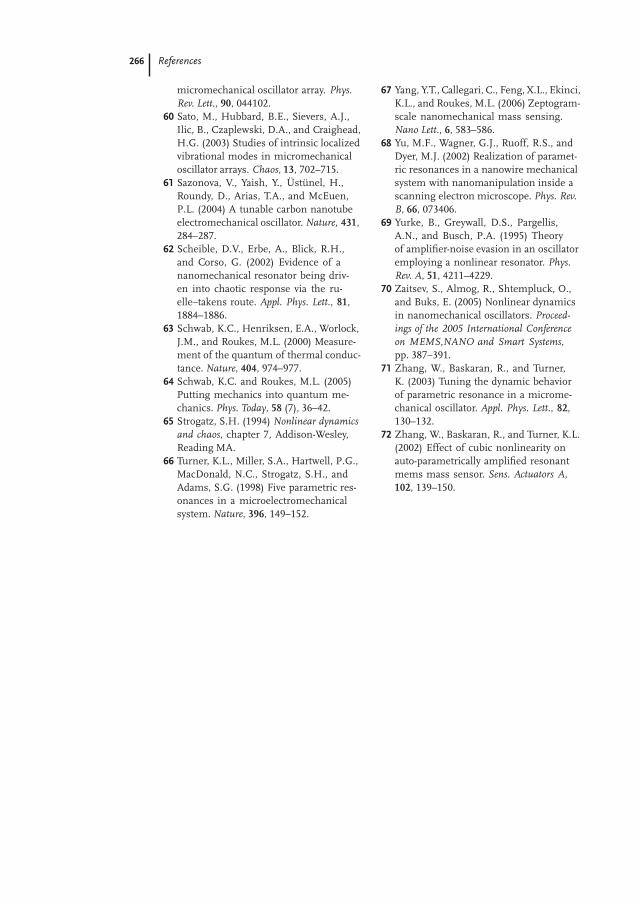
266 References
micromechanical oscillator array. Phys.
Rev. Lett., 90, 044102.60 Sato, M., Hubbard, B.E., Sievers, A.J.,
Ilic, B., Czaplewski, D.A., and Craighead,H.G. (2003) Studies of intrinsic localizedvibrational modes in micromechanicaloscillator arrays. Chaos, 13, 702–715.
61 Sazonova, V., Yaish, Y., Üstünel, H.,Roundy, D., Arias, T.A., and McEuen,P.L. (2004) A tunable carbon nanotubeelectromechanical oscillator. Nature, 431,284–287.
62 Scheible, D.V., Erbe, A., Blick, R.H.,and Corso, G. (2002) Evidence of ananomechanical resonator being driv-en into chaotic response via the ru-elle–takens route. Appl. Phys. Lett., 81,1884–1886.
63 Schwab, K.C., Henriksen, E.A., Worlock,J.M., and Roukes, M.L. (2000) Measure-ment of the quantum of thermal conduc-tance. Nature, 404, 974–977.
64 Schwab, K.C. and Roukes, M.L. (2005)Putting mechanics into quantum me-chanics. Phys. Today, 58 (7), 36–42.
65 Strogatz, S.H. (1994) Nonlinear dynamics
and chaos, chapter 7, Addison-Wesley,Reading MA.
66 Turner, K.L., Miller, S.A., Hartwell, P.G.,MacDonald, N.C., Strogatz, S.H., andAdams, S.G. (1998) Five parametric res-onances in a microelectromechanicalsystem. Nature, 396, 149–152.
67 Yang, Y.T., Callegari, C., Feng, X.L., Ekinci,K.L., and Roukes, M.L. (2006) Zeptogram-scale nanomechanical mass sensing.Nano Lett., 6, 583–586.
68 Yu, M.F., Wagner, G.J., Ruoff, R.S., andDyer, M.J. (2002) Realization of paramet-ric resonances in a nanowire mechanicalsystem with nanomanipulation inside ascanning electron microscope. Phys. Rev.
B, 66, 073406.69 Yurke, B., Greywall, D.S., Pargellis,
A.N., and Busch, P.A. (1995) Theoryof amplifier-noise evasion in an oscillatoremploying a nonlinear resonator. Phys.
Rev. A, 51, 4211–4229.70 Zaitsev, S., Almog, R., Shtempluck, O.,
and Buks, E. (2005) Nonlinear dynamicsin nanomechanical oscillators. Proceed-
ings of the 2005 International Conference
on MEMS,NANO and Smart Systems,pp. 387–391.
71 Zhang, W., Baskaran, R., and Turner,K. (2003) Tuning the dynamic behaviorof parametric resonance in a microme-chanical oscillator. Appl. Phys. Lett., 82,130–132.
72 Zhang, W., Baskaran, R., and Turner, K.L.(2002) Effect of cubic nonlinearity onauto-parametrically amplified resonantmems mass sensor. Sens. Actuators A,102, 139–150.