8. assessment of the flathead sole stock in the gulf of alaska
TRANSCRIPT

8. Assessment of the Flathead Sole Stock in the Gulf of Alaska
By
Carey R. McGilliard1, Wayne Palsson3, William Stockhausen2, and Jim Ianelli2
1Joint Institute for the Study of the Atmosphere and Ocean University of Washington
Seattle, WA 98195 2Resource Ecology and Fisheries Management Division
3Resource Assessment and Conservation Engineering Division Alaska Fisheries Science Center
National Marine Fisheries Service National Oceanic and Atmospheric Administration
7600 Sand Point Way NE., Seattle, WA 98115-6349
EXECUTIVE SUMMARY
Summary of Changes in Assessment Inputs
(1) 1978-1983 and 2012-2013 catch data were included in the model
2011 catch was updated to include October – December catch in that year
(2) 2012 and 2013 fishery length composition data were added to the model (3) 1985-1988, 2000, and 2008 fishery length composition data were excluded from the model due to low
sample size (4) The number of hauls was used as the effective sample size of fishery length-composition data (5) The range of length bins was expanded such that the lowest length bin included 0-6cm fish and the
oldest bin included 70cm+ fish. (6) The 2013 survey biomass index was added to the model (7) Survey length composition data for 2013 were added to the model (8) Survey age composition data within each length bin were used in the model instead of marginal age
composition data (combined over lengths); 2011 age composition data (within each length bin) were added to the model.
(9) The “plus” group was increased to age 29.
Summary of Changes in Assessment Methodology
The following substantive structural changes were made to the assessment methodology:
(1) The assessment was conducted in Stock Synthesis version 3.14o (SS3); Attachment 8B includes a full description of the transition from the 2011 flathead sole assessment model to an equivalent model in SS3.
(2) The fishery and survey selectivity curves were estimated using an age-based double-normal function without a descending limb instead of an age-based logistic function.
(3) A conditional age-at-length likelihood approach was used: expected age composition within each length bin was fit to age data conditioned on length in the likelihood function, rather than fitting the expected marginal age-composition to age data that weren’t conditioned on length.
(4) Parameters of the von-Bertlanffy growth curve were estimated within the model. (5) The CVs of length at age 2 and 29 were estimated within the model and used to define the age-length
transition matrix. (6) Initial equilibrium F was estimated within the model

(7) Relative weights of composition data were adjusted according to the data-weighting method described in Francis (2011).
(8) Ageing uncertainty was incorporated into the model using the ageing error matrix used in the most recent accepted BSAI flathead sole assessment.
(9) Recruitment deviations prior to 1984 were estimated as “early-period” recruits separately from main-period recruits (1984-2008) such that the vector of recruits for each period had a sum-to-zero constraint, rather than forcing a sum-to-zero constraint across all recruitment deviations.
Summary of Results
The key results of the assessment, based on the author’s preferred model, are compared to the key results of the accepted 2011 assessment model in the table below.
M (natural mortality rate) 0.2 0.2 0.2 0.2Tier 3a 3a 3a 3aProjected total (3+) biomass (t) 288,538 285,128 252,361 253,418Female spawning biomass (t) Projected Upper 95% confidence interval -- 84,076 83,287 Point estimate 106,377 107,178 84,058 83,204 Lower 95% confidence interval -- 84,045 83,141
B 100% 103,868 103,868 88,829 88,829
B 40% 41,547 41,547 35,532 35,532
B 35% 36,354 36,354 31,090 31,090
F OFL 0.593 0.593 0.61 0.61
maxF ABC 0.45 0.45 0.47 0.47
F ABC 0.45 0.45 0.47 0.47OFL (t) 61,036 62,296 50,664 50,376maxABC (t) 48,738 49,771 41,231 41,007ABC (t) 48,738 49,771 41,231 41,007
2011 2012 2012 2013Overfishing no n/a no n/aOverfished n/a no n/a noApproaching overfished n/a no n/a no
StatusAs determined in 2012 for: As determined in 2013 for:
Quantity
As estimated orspecified last year for:
As estimated orrecommended this year for:
2013 2014 2014 2015

The table below shows apportionment of the 2014 and 2015 ABCs and OFLs among areas, based on the percentage of flathead sole 2013 survey biomass in each area.
Responses to SSC and Plan Team Comments on Assessments
Due to the October government shutdown, Alaska Fisheries Science Center (AFSC) leadership has determined that responses to Plan Team and SSC comments were optional for this year’s stock assessments. The following issues were addressed.
GPT (11/11 minutes): “The Team noted the model starts in 1984 rather than 1977. Since catches prior to 1984 are presented in the assessment, the Team recommends the author attempt to start the model in 1977 to be consistent with other stock assessments”. Catches from 1978-1983 were included in the model. The 2013 model starts in 1978 and an initial equilibrium catch is estimated to account for fishing prior to 1978.
GPT (11/11 minutes): “The Team also recommends the author work to incorporate an ageing error matrix for flathead sole for use in the model”. Ageing uncertainty was incorporated into the model using the ageing error matrix calculated from BSAI flathead sole ageing data and used in the most recent accepted BSAI flathead sole assessment. Future assessments should estimate an ageing error matrix using GOA flathead ageing error data.
GPT (11/11 mintues):“The Team recommends the model be configured to accept fishery ages and that the author evaluate available sample sizes and work with the ageing lab to get additional ages processed”. The SS3 model framework used for the 2013 assessment is configured to accept fishery ages. The author is working with the ageing lab to get additional ages processed so that fishery ages can be used in future assessments.
SSC (12/11 minutes): The SSC supports the authors’ plans to estimate new age-length transition matrices with newly available age data. Age-length transition matrices with newly available age data were evaluated within the assessment model by estimating the parameters of the von-Bertalanffy growth curve and the CV of length-at-age for the youngest and oldest fish in the population (from which an age-length transition matrix was calculated). All available survey age-at-length data were included in the model to inform the estimation of growth and age-length transition matrices.
SSC (12/11 minutes): The SSC asks the authors to consider whether an analysis of aging error would be timely either by the AFSC’s Age and Growth Program or internal to the model or both. Ageing uncertainty was incorporated into the model using the ageing error matrix calculated from BSAI flathead sole ageing data and used in the most recent accepted BSAI flathead sole assessment. Future assessments should estimate an ageing error matrix using GOA flathead ageing error data.
GPT (9/13 minutes): The Team recommended that the author continue to use the stock synthesis framework for both species since it can accommodate past issues that have been raised. Also fits to the survey index data were much better. The Stock Synthesis framework was used for the current assessment.
Quantity Western CentralWest
Yakutat Southeast Total
Area Apportionment 30.88% 60.16% 8.55% 0.41% 100.00%
2014 ABC (t) 12,730 24,805 3,525 171 41,231
2015 ABC (t) 12,661 24,670 3,506 170 41,007

SSC (10/13 minutes): The SSC recommends that the previous stock assessment platforms be updated with the most current data for comparison to the new SS models before transition to the new SS platform. Attachment 8B of the assessment shows the results of model runs using the previous stock assessment platform, updated with the most current data and compares model results to those of the current assessment using the new SS platform.
INTRODUCTION
General
Flathead sole (Hippoglossoides elassodon) are distributed from northern California, off Point Reyes, northward along the west coast of North America and throughout the GOA and the BS, the Kuril Islands, and possibly the Okhotsk Sea (Hart 1973). They occur primarily on mixed mud and sand bottoms (Norcross et al. 1997, McConnaughey and Smith 2000) in depths < 300 m (Stark and Clausen 1995). The flathead sole distribution overlaps with the similar-appearing Bering flounder (Hippoglossoides robustus) in the northern half of the Bering Sea and the Sea of Okhotsk (Hart 1973), but not in the Gulf of Alaska.
Review of Life History
Adults exhibit a benthic lifestyle and occupy separate winter spawning and summertime feeding distributions on the EBS shelf and in the GOA. From over-winter grounds near the shelf margins, adults begin a migration onto the mid and outer continental shelf in April or May each year for feeding. The spawning period may range from as early as January but is known to occur in March and April, primarily in deeper waters near the margins of the continental shelf. Eggs are large (2.75 to 3.75 mm) and females have egg counts ranging from about 72,000 (20 cm fish) to almost 600,000 (38 cm fish). Eggs hatch in 9 to 20 days depending on incubation temperatures within the range of 2.4 to 9.8°C and have been found in ichthyoplankton sampling on the southern portion of the BS shelf in April and May (Waldron 1981). Larvae absorb the yolk sac in 6 to 17 days, but the extent of their distribution is unknown. Nearshore sampling indicates that newly settled larvae are in the 40 to 50 mm size range (Norcross et al. 1996). Fifty percent of flathead sole females in the GOA are mature at 8.7 years, or at about 33 cm (Stark 2004). Juveniles less than age 2 have not been found with the adult population and probably remain in shallow nearshore nursery areas.
FISHERY
Description of the Directed Fishery
Flathead sole in the Gulf of Alaska are caught in a directed fishery using bottom trawl gear. Typically 25 or fewer shore-based catcher vessels from 58-125’ participate in this fishery, as do 5 catcher-processor vessels (90-130’). Fishing seasons are driven by seasonal halibut PSC apportionments, with approximately 7 months of fishing occurring between January and November. Catches of flathead sole occur only in the Western and Central management areas in the gulf (statistical areas 610 and 620 + 630, respectively, Figure 8.2-Figure 8.6). Recruitment to the fishery begins at about age 3.
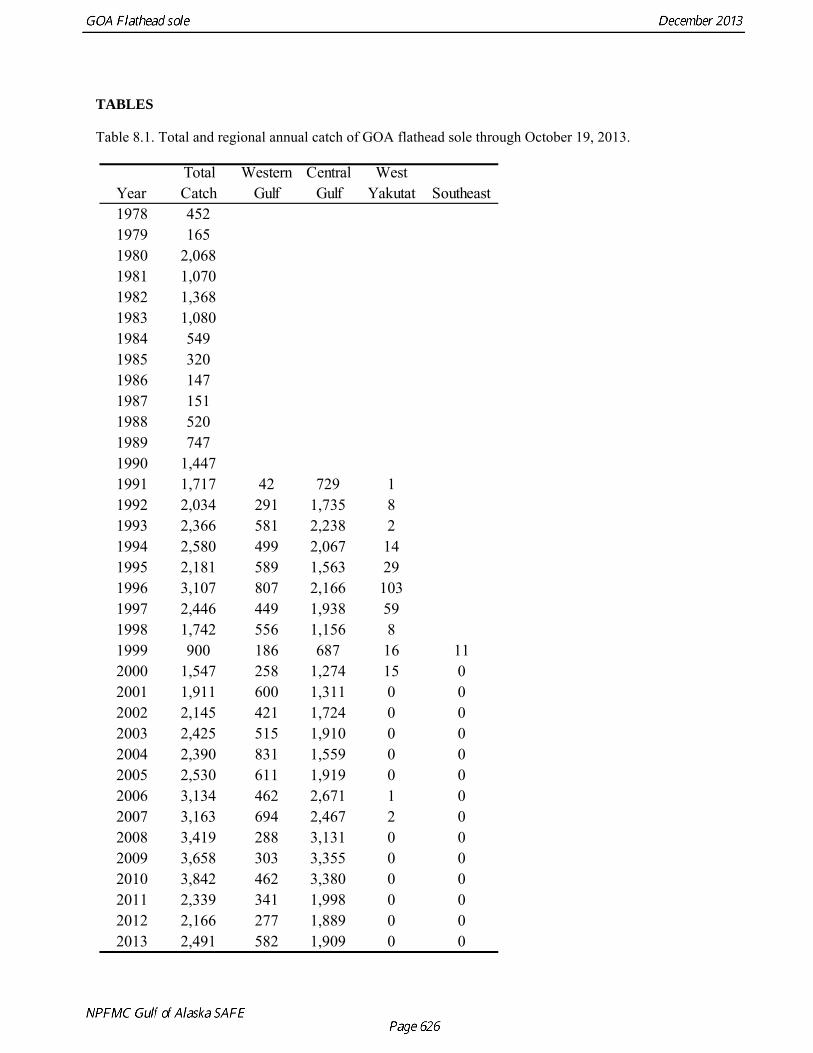
Historically, catches of flathead sole have exhibited decadal-scale trends (Table 8.1, Figure 8.1). From a high of ~2000 t in 1980, annual catches declined steadily to a low of ~150 t in 1986 but thereupon increased steadily, reaching a high of ~3100 t in 1996. Catches subsequently declined over the next three years, reaching a low of ~900 t in 1999, followed by an increasing trend through 2010, when the catch reached its highest level ever (3,842 t).

Based on observer data, the majority of the flathead sole catch in the Gulf of Alaska is taken in the Shelikof Strait and on the Albatross Bank near Kodiak Island, as well as near Unimak Island (Stockhausen 2011). Previously, most of the catch is taken in the first and second quarters of the year (Stockhausen 2011).
Annual catches of flathead sole have been well below TACs in recent years (Table 8.2), although the population appears to be capable of supporting higher exploitation rates. Limits on flathead sole catches are driven by within-season closures of the directed fishery due to restrictions on halibut PSC, not by attainment of the TAC (Stockhausen 2011).
See Stockhausen (2011) for a description of the management history of flathead sole.
DATA
The following table specifies the source, type, and years of all data included in the assessment models.
Source Type Years
Fishery Catch biomass 1978-2013
Fishery Catch length composition 1989-1999, 2001-2007, 2009-2013
GOA survey bottom trawl
Catch per unit effort Triennial: 1984-1999, Biennial: 2001-2013
GOA survey bottom trawl
Catch length composition Triennial: 1984-1999, Biennial: 2001-2013
GOA survey bottom trawl
Catch age composition, conditioned on length
Triennial: 1984-1999, Biennial: 2001-2013
Fishery Data
Catch Biomass
The assessment included catch data from 1978 to October 19, 2013 (Table 8.1, Figure 8.1). Fishery catch per unit effort (CPUE) data are excluded because flathead sole are often taken as incidental catch and it is thought that the fishery CPUE data may not reflect abundance. The spatial distribution of fishery CPUE for 2009-2013 is shown in Figure 8.2-Figure 8.6.
Catch Size Composition
Fishery length composition data were included in 2cm bins from 6-56cm in 1989-1999, 2001-2007, and 2009-2013; data were omitted in years where there were less than 15 hauls that included measured flathead sole (1982-1988 2000, 2008). The number of hauls were used as the relative effective sample size. Fishery length composition data were voluminous and can be accessed at http://www.afsc.noaa.gov/REFM/docs/2013/GOA_Flathead_Composition_Data_And_SampleSize_2013.xlsx.

GOA Survey Bottom Trawl Data
Biomass and Numerical Abundance
Survey biomass estimates originate from a cooperative bottom trawl survey between the U.S. and Japan in 1984 and 1987 and a U.S. bottom trawl survey conducted by the Alaska Fisheries Science Center Resource Assessment and Conservation Engineering (RACE) Division thereafter. Calculations for final survey biomass and variance estimates are fully described in Wakabayashi et al. (1985). Depths 0-500 meters were fully covered in each survey and occurrence of flathead at depths greater than 500 meters is rare. The survey excluded the eastern part of the Gulf of Alaska (the Yakutat and Southeastern areas) in 2001 (Table 8.3). As for previous assessments, the availability of the survey biomass in 2001 was assumed to be 0.9 to account for the biomass in the eastern section of the Gulf. The total survey biomass estimates and CVs that were used in the assessment are listed in Table 8.4.
Figure 8.7-Figure 8.9 show maps of survey CPUE in the GOA for the 2009, 2011, and 2013 surveys; survey CPUE in all three years was highest in the Central and Western GOA.
Survey Size and Age Composition
Sex-specific survey length composition data as well as age frequencies of fish by length (conditional age-at-length) were used in the assessment and can be found at http://www.afsc.noaa.gov/REFM/docs/2013/GOA_Flathead_Composition_Data_And_SampleSize_2013.xlsx, along with corresponding sample sizes used in the assessment. There are several advantages to using conditional age-at-length data. The approach preserves information on the relationship between length and age and provides information on variability in length-at-age such that growth parameters and variability in growth can be estimated within the model. In addition, the approach resolves the issue of double-counting individual fish when using both length- and age-composition data (as length-composition data are used to calculate the marginal age compositions). See Stewart (2005) for an additional example of the use of conditional age-at-length data in fishery stock assessments.
ANALYTICAL APPROACH
Model Structure
Tier 3 Model
The assessment was a split sex, age-structured statistical catch-at-age model implemented in Stock Synthesis version 3.24o (SS3) using a maximum likelihood approach. SS3 equations can be found in Methot and Wetzel (2013) and further technical documentation is outlined in Methot (2009). Previous assessments were conducted using an ADMB-based, split-sex, age-structured population dynamics model (Stockhausen 2011). Briefly, the current assessment model covers 1955-2013. Age classes included in the model run from age 0 to 29. Age at recruitment was set at 0 years in the model. The oldest age class in the model, age 29, serves as a plus group. Survey catchability was fixed at 1.0. A detailed description of the transition of the previous model to SS3 and potential benefits of transitioning the assessment to SS3 were presented at the 2013 September Plan Team Meeting and the September SAFE chapter is included in this document as Attachment 8A.
Fishery and Survey Selectivity
The fishery and survey selectivity curves were estimated using sex-specific, age-based double-normal functions without a descending limb (instead of a logistic function). The SS3 modeling framework does

not currently include the option of estimating sex-specific, age-based logistic selectivity where both male and female selectivity maintain a logistic shape (as was used in the previous assessment model). Therefore, the double-normal curve without a descending limb was the closest match to the selectivity formulation used in the 2011 model (Attachment 8A). Length-based, sex-specific, logistic fishery and survey selectivity were implemented as sensitivity analyses in 2013 assessment model runs (Attachment 8A). Length-based formulations for fishery and survey selectivity were not used in final model runs because the age-based selectivity curves derived from using length-based curves showed that the oldest fish were not selected, effectively lowering survey catchability and suggesting that the fishery fails to catch the oldest, largest fish. Fits to data were similar for length- and age-based asymptotic survey selectivity curves. Sensitivity analyses assuming dome-shaped fishery or survey selectivity failed to improve model fits to the data.
Conditional Age-at-Length
A conditional age-at-length approach was used: expected age composition within each length bin was fit to age data conditioned on length (conditional age-at-length) in the objective function, rather than fitting the expected marginal age-composition to age data (which are typically calculated as a function of the conditional age-at-length data and the length-composition data). This approach provides the information necessary to estimate growth curves and variability about mean growth within the assessment model. In addition, the approach allows for all of the length and age-composition information to be used in the assessment without double-counting each sample. The von-Bertalanffy growth curve and variability in the length-at-age relationship were evaluated within the model using the conditional age-at-length approach.
Data Weighting
In the 2011 assessment, data components within the model were weighted as follows:
Fishery Catch
Fishery Length
Survey Biomass
Survey Length
Survey Age
30 1 1 1 1
The GOA Plan Team expressed concerns about effective sample sizes and data weighting used in the previous assessment. Therefore, in the current assessment, effective sample sizes for fishery length-composition data each year were set to the number of hauls measured to account for non-independence within hauls (Pennington and Volstad 1994). The effective sample sizes for survey length-composition data were the same in each survey year (as for previous assessments). Future assessments should explore intra-haul correlation and the possibility of using number of hauls for effective sample size of survey length-composition data (Pennington and Volstad 1994). To account for process error (e.g. variance in selectivities among years), relative weights measured for length or age composition data (lambdas) were adjusted according to the method described in Francis (2011), which accounts for correlations in length- and age-composition data (data-weighting method number T3.4 was used). The weights used were
for the fishery length composition data, for the survey length-composition data,
for the survey age composition data, and for the survey biomass index. The
philosophy of this data-weighting method is to avoid allowing age- and length-composition data to prevent the model from fitting the survey biomass data well and to account for correlations in the residuals about the fits to the length- and age-composition data (Francis 2011). Previous studies show that solely using composition data to determine trends in biomass can lead to widely varying conclusions about current biomass and biomass reference points (Horn and Francis 2010).
0.081 2.191 0.653 1

Ageing Error Matrix
Ageing uncertainty was incorporated into the model using the ageing error matrix calculated from BSAI flathead sole ageing data and used in the most recent accepted BSAI flathead sole assessment (Stockhausen et al. 2012). SS3 accommodates the specification of ageing error bias and imprecision, while the previous assessment model framework did not. Future assessments should estimate ageing error matrices for GOA flathead sole using GOA age-read data. BSAI and GOA flathead sole are aged by the same individuals using the same techniques and ageing error is expected to be very similar. Assuming perfect age-reading of GOA flathead sole otoliths is thought to be an inferior assumption to using estimates of ageing error from the BSAI flathead sole population. The BSAI data was used due to insufficient time to properly analyze GOA ageing error data.
Recruitment Deviations
Recruitment deviations for the period 1955-1983 were estimated as “early-period” recruits separately from “main-period” recruits (1984-2008) such that the vector of recruits for each period had a sum-to-zero constraint, rather than forcing a sum-to-zero constraint across all recruitment deviations.
A bias adjustment factor was specified using the Methot and Taylor (2011) bias adjustment method. Recruitment deviations prior to the start of composition data and in the most recent years in the time-series are less informed than in the middle of the time-series. This creates a bias in the estimation of recruitment deviations and mean recruitment that is corrected using methods described in Methot and Taylor (2011).
Model structures considered in this year’s assessment
Many proposed model changes were presented at the 2013 September Plan Team meeting (Attachment 8A) and were explored using 2012-2013 data. The four models described below are included in the final assessment; all use the SS3 model framework and include nearly all of the changes that were proposed and reviewed at the September Plan Team meeting (Attachment 8A). Survey catchability is fixed and equal to 1 for all models.
Model 0 (the author’s recommended model) implemented the changes described above, fixing natural mortality at 0.2 for males and females, the value specified in the previous assessment. When natural mortality is fixed and equal to 0.2, a constraint is placed on the fishery selectivity curves such that selectivity reaches 1 by age 16. Growth curves for flathead sole indicate that flathead have reached maximum length by age 16. Recruitment deviations for an “early” time period from 1955-1983 (prior to the availability of composition data) were estimated, as described above. Estimating early-period recruitment deviations allows the model to fit to the initial age-composition data.
Model 1 is as for Model 0, but with male and female natural mortality (M) estimated. Model fits and the ability to estimate reasonable fishery selectivity curves improved substantially when natural mortality was estimated. Like Model 0, Model 1 recruitment deviations for the “early” time period from 1955-1983 were estimated.
Model 2 is as for Model 0, but a different R0 value was estimated prior to 1984, and recruitment deviations were estimated starting in 1984. Excluding the early-period recruitment deviations prevents the model from estimating extreme values for early-period recruitment deviations when data to support these estimates are sparse. As for Model 0, fishery selectivity was constrained such that selectivity reached 1 by age 16 and natural mortality was fixed and equal to 0.2 for males and females.

Model 3 is as for Model 1, where male and female natural mortality are estimated, but excluded the estimation of early-period recruits and instead estimated a different R0 value during the early period. Recruitment deviations were estimated beginning in 1984.
Parameters Estimated Outside the Assessment Model
Natural mortality
Male and female natural mortality were fixed and equal to 0.2 in Models 0 and 2.
Weight-Length Relationship
The weight-length relationship was that used in the previous assessment (Stockhausen 2011). The
relationship was Lw L , where 4.28 06E and 3.2298 , length (L) was measured in
centimeters and weight (w) was measured in kilograms.
Maturity-at-Age
Maturity-at-age ( )aO in the assessment was defined as 50( )1/ (1 )a aaO e , where the slope of the
curve was 0.773 and the age-at-50%-maturity was 50 8.74a . These values were used in the
previous assessment and were estimated from a histological analysis of GOA flathead sole ovaries collected in January 1999 based on 180 samples (Stark, 2004).
Standard deviation of the Log of Recruitment ( R )
The standard deviation of the log of recruitment was not defined in previous assessments. Variability of the recruitment deviations that were estimated in previous flathead sole assessments was approximately
R =0.6 and this value was used in the current assessment.
Catchability
Catchability was equal to 1, as for previous flathead sole assessments.
Select selectivity parameters
Selectivity parameter definitions and values are shown in Table 8.5.
Parameters Estimated Inside the Assessment Model
Parameters estimated within the assessment model were natural mortality (Models 1 and 3 only), the log of unfished recruitment (R0), log-scale recruitment deviations, yearly fishing mortality, sex-specific parameters of the von-Bertalanffy growth curve, CV of length-at-age for ages 2 and 29, and selectivity parameters for the fishery and survey. The selectivity parameters are described in greater detail in Table 8.5.

RESULTS
Model Evaluation
Comparison among models
Models with estimated M (Models 1 and 3) led to reasonable estimates of selectivity parameters without constraining parameters (Figure 8.16, Figure 8.18), while models with fixed M (Models 0 and 2) required a constraint such that selectivity would reach 1 before the age of the plus group. Specifically, the constraint imposed for models with fixed M was that selectivity must reach 1 by age 16 (when most fish were fully grown; Figure 8.15, Figure 8.17). Without this constraint, models with M = 0.2 led to estimated selectivity curves with very shallow slopes, reaching maximum selectivity at age 37; the plus group age is 29 (Figure 8.19).
Models where M was estimated (Models 1 and 3) produced the best total negative log likelihood values due to improvements in fits to length- and age-composition data (Table 8.6). Figure 8.20-Figure 8.23 show observed and predicted proportions-at-length, aggregated over years. Models 1 and 3, where M was estimated, led to better fits of both the fishery and survey female proportions-at-length. Predicted male proportions-at-length fit the data closely and fits were similar across the four alternative models. Fits to the survey biomass index were similar among models, but slightly worse for models where M was estimated (Table 8.6, Figure 8.11). Models with estimated M predicted higher survey biomass and spawning stock biomass in early years of the time series and very similar, but slightly lower survey biomass in later years than models with fixed M (Figure 8.11-Figure 8.12).
Estimates of male and female M were higher than 0.2, the values used in previous assessments (Model 1 M= 0.287 (females) and 0.217 (males) and Model 3 M= 0.291 (females) and 0.321 (males); Table 8.7). Higher estimates of M led to substantially higher estimates of age-0 recruitment (Figure 8.14) and unfished recruitment (Table 8.7). The models with estimated M led to broader uncertainty intervals in estimates of spawning biomass, as expected (Figure 8.12). Estimates of spawning biomass were similar among models (Figure 8.12).
Models 0 and 1 include estimates of early recruitment deviations from 1955 to 1983, prior to the start of the length- and age-composition data. A pattern of negative recruitment deviations occurred from 1955 until the mid-1970s, when a spike in positive recruitment deviations occurred (Figure 8.13). This pattern occurred for every exploratory model run that included early-period recruitment deviations. When comparing between models that differed only in estimation of early recruitment deviations (i.e. comparing Model 0 to Model 2 and Model 1 to Model 3), length- and age-composition likelihood components and total negative log likelihood values were slightly better for models with early-period recruitment deviations than for models without early-period deviations (Table 8.6). It is expected that estimating early recruitment deviations would improve the total negative log likelihood and specifically the fits to composition data because the sole purpose is to allow the model more freedom to specify an initial age composition.
The Author’s Recommended Model (Model 0)
The model recommended by the author is Model 0 where natural mortality was fixed to the value used in previous assessments (0.2) and early period recruitment deviations were estimated. Model 0 was selected for two reasons.
(1) Excluding initial recruitment deviations forces an assumption that the age-structure of the population is at a fished equilibrium in 1984. This assumption seems less realistic than the possibility of a large

recruitment pulse in the 1970s, as fish recruitment is known to fluctuate. The magnitude of recruitment deviations in the early period is similar to that of the main-period recruitment deviations in models with estimated M. The smoothness of the pattern in early recruitment deviations can largely be attributed to the inclusion of ageing error in the model, such that the model may be able to identify that a large recruitment pulse occurred, but can’t identify the exact year or years of the recruitment pulse.
(2) While the models with estimated natural mortality (Models 1 and 3) were a better fit to the data than the models where natural mortality was set equal to 0.2, natural mortality and catchability may be confounded. Future assessments should explore both the possibility that GOA flathead sole natural mortality is higher than is being assumed and whether catchability may be lower than 1. The substantial improvement in fits to the data and the ability of the model to estimate reasonable fishery selectivity curves when natural mortality is estimated is notable and should be considered in future assessments.
Figure 8.20 and Figure 8.24-Figure 8.29 show fits to the aggregated and yearly proportions-at-age data for the fishery and the survey. Fits to male fishery and survey proportion-at-length data were reasonable. Fits to female fishery proportion-at-length data were generally shifted slightly towards smaller lengths and estimated survey proportions-at-length predicted a smaller proportion of females in the 30-40 cm length bins. Figure 8.30 and Table 8.12 shows the length-at-age relationship estimated by Model 0 and Figure 8.31 shows growth relationships for Model 0 in comparison to those used in previous assessments. Estimates of growth were very similar to those obtained in previous assessments from estimating growth outside of the assessment model. Figure 8.32-Figure 8.37 show that fits to age-at-length data are reasonable, as most expected ages-at-length match the mean of the observed values in most years. An exception is expected female age-at-length in 2011, where expected mean age at older lengths is greater than the observed mean age. The expected standard deviation of age-at-length (right column, Figure 8.32-Figure 8.37) is sometimes very different from the observed standard deviation at large lengths. This is a result of low sample sizes in the largest length bins: the observed standard deviation in a length bin will be 0 if only 1 fish in that bin was aged; the expected standard deviation in age-at-length is calculated based on the entire expected number of fish at a given length in the estimated population.
Yearly estimates of fishing mortality rates are reported in Table 8.11.
Additional plots of Model 1 were provided to show the improved fits to length-composition and conditional age-at-length data when natural mortality was estimated (Figure 8.40-Figure 8.54). In addition, Figure 8.54 shows a phase plot based on Model 1 to show implications of the higher values estimated for natural mortality on the model’s interpretation of stock status and fishing mortality over time, relative to key reference points.
Time Series Results
Time series results are shown in Table 8.13-Table 8.14 and Figure 8.38-Figure 8.39. A time series of numbers at age is available at http://www.afsc.noaa.gov/REFM/docs/2013/GOA_Flathead_TimeSeries_of_NumbersAtAge_2013.xlsx. Age 3 recruitment, age 0 recruitment, and standard deviations of age 0 recruitment are presented in Table 8.13 for the previous and current assessments. Total biomass for ages 3+, spawning stock biomass, and standard deviations of spawning stock biomass estimates for the previous and current assessments are presented in Table 8.14. Figure 8.38 shows spawning stock biomass estimates and corresponding asymptotic 95% confidence intervals. Figure 8.39 is a plot of biomass relative to B35% and F relative to F35% for each year in the time series, along with the OFL and ABC control rules.

HARVEST RECOMMENDATIONS
The reference fishing mortality rate for flathead sole is determined by the amount of reliable population information available (Amendment 56 of the Fishery Management Plan for the groundfish fishery of the Bering Sea/Aleutian Islands). Estimates of F40%, F35%, and SPR40% were obtained from a spawner-per recruit analysis. Assuming that the average recruitment from the 1983-2010 year classes estimated in this assessment represents a reliable estimate of equilibrium recruitment, then an estimate of B40% is calculated as the product of SPR40% times the equilibrium number of recruits. Since reliable estimates of the 2013 spawning biomass (B), B40%, F40%, and F35% exist and B>B40%, the flathead sole reference fishing mortality is defined in Tier 3a. For this tier, FABC is constrained to be ≤ F40%, and FOFL is defined to be F35%. The values of these quantities are:
Because the flathead sole stock has not been overfished in recent years and the stock biomass is relatively high, it is not recommended to adjust FABC downward from its upper bound.
A standard set of projections is required for each stock managed under Tiers 1, 2, or 3 of Amendment 56. This set of projections encompasses seven harvest scenarios designed to satisfy the requirements of Amendment 56, the National Environmental Policy Act, and the Magnuson-Stevens Fishery Conservation and Management Act (MSFCMA). For each scenario, the projections begin with the vector of 2013 numbers at age estimated in the assessment. This vector is then projected forward to the beginning of 2014 using the schedules of natural mortality and selectivity described in the assessment and the best available estimate of total (year-end) catch for 2013. In each subsequent year, the fishing mortality rate is prescribed on the basis of the spawning biomass in that year and the respective harvest scenario. In each year, recruitment is drawn from an inverse Gaussian distribution whose parameters consist of maximum likelihood estimates determined from recruitments estimated in the assessment. Spawning biomass is computed in each year based on the time of peak spawning and the maturity and weight schedules described in the assessment. Total catch is assumed to equal the catch associated with the respective harvest scenario in all years. This projection scheme is run 1000 times to obtain distributions of possible future stock sizes, fishing mortality rates, and catches.
Five of the seven standard scenarios will be used in an Environmental Assessment prepared in conjunction with the final SAFE. These five scenarios, which are designed to provide a range of harvest alternatives that are likely to bracket the final TAC for 2014, are as follow (“max FABC” refers to the maximum permissible value of FABC under Amendment 56):
Scenario 1: In all future years, F is set equal to max FABC. (Rationale: Historically, TAC has been constrained by ABC, so this scenario provides a likely upper limit on future TACs.)
SSB 2013 84,058
B 40% 35,532
F 40% 0.47
maxFabc 0.47
B 35% 31,090
F 35% 0.61
F OFL 0.61

Scenario 2: In all future years, F is set equal to a constant fraction of max FABC, where this fraction is equal to the ratio of the FABC value for 2014 recommended in the assessment to the maxFABC for 2014. (Rationale: When FABC is set at a value below max FABC, it is often set at the value recommended in the stock assessment.)
Scenario 3: In all future years, F is set equal to 50% of max FABC. (Rationale: This scenario provides a likely lower bound on FABC that still allows future harvest rates to be adjusted downward when stocks fall below reference levels.)
Scenario 4: In all future years, F is set equal to the 2008-2013 average F. (Rationale: For some stocks, TAC can be well below ABC, and recent average F may provide a better indicator of FTAC than FABC.)
Scenario 5: In all future years, F is set equal to zero. (Rationale: In extreme cases, TAC may be set at a level close to zero.) The recommended FABC and the maximum FABC are equivalent in this assessment, so scenarios 1 and 2 yield identical results. The 12-year projections of the mean spawning stock biomass, fishing mortality, and catches for the five scenarios are shown in Table 8.15Table 8.17.
Two other scenarios are needed to satisfy the MSFCMA’s requirement to determine whether the flathead sole stock is currently in an overfished condition or is approaching an overfished condition. These two scenarios are as follows (for Tier 3 stocks, the MSY level is defined as B35%):
Scenario 6: In all future years, F is set equal to FOFL. (Rationale: This scenario determines whether a stock is overfished. If the stock is expected to be above its MSY level in 2014, then the stock is not overfished.)
Scenario 7: In 2014 and 2015, F is set equal to max FABC, and in all subsequent years, F is set equal to FOFL. (Rationale: This scenario determines whether a stock is approaching an overfished condition. If the stock is expected to be above its MSY level in 2026 under this scenario, then the stock is not approaching an overfished condition.)
The results of these two scenarios indicate that the stock is not overfished and is not approaching an overfished condition. With regard to assessing the current stock level, the expected stock size in the year 2014 of scenario 6 is 84,059 t, more than 2 times B35% (31,090 t). Thus the stock is not currently overfished. With regard to whether the stock is approaching an overfished condition, the expected spawning stock size in the year 2026 of scenario 7 (32,701 t) is greater than B35%; thus, the stock is not approaching an overfished condition.
Area Allocation of Harvests
TAC’s for flathead sole in the Gulf of Alaska are divided among four smaller management areas (Western, Central, West Yakutat and Southeast Outside). As for previous assessments, the area-specific ABC’s for flathead sole in the GOA are divided up over the four management areas by applying the fraction of the most recent survey biomass estimated for each area (relative to the total over all areas) to the 2014 and 2015 ABC’s. The area-specific allocations for 2014 and 2015 are:

SOURCES CITED
Francis, R. I. C. C. 2011. Data weighting in statistical fisheries stock assessment models. Canadian Journal of Fisheries and Aquatic Sciences 68:1124-1138.
Hart, J. L. 1973. Pacific fishes of Canada. Fish Res. Board Canada, Bull. No. 180. 740 p. Horn and R. I. C. C. Francis. 2010. Stock assessment of hake (Merluccius australis) on the
Chatham Rise for the 2009–10 fishing year. New Zealand Fisheries Assessment Report 2010/14, Ministry of Fisheries, Wellington, New Zealand.
McConnaughey, R. A. and K. R. Smith. 2000. Associations between flatfish abundance and surficial sediments in the eastern Bering Sea. Canadian Journal of Fisheries and Aquatic Sciences 57:2410-2419.
Methot, R. D. 2009. User manual for stock synthesis, model version 3.04b. NOAA Fisheries, Seattle, WA.
Methot, R. D. and I. G. Taylor. 2011. Adjusting for bias due to variability of estimated recruitments in fishery assessment models. Canadian Journal of Fisheries and Aquatic Sciences 68:1744-1760.
Methot, R. D. and C. R. Wetzel. 2013. Stock synthesis: A biological and statistical framework for fish stock assessment and fishery management. Fisheries Research 142:86-99.
Norcross, B. L., B. A. Holladay, S. C. Dressel, and M. Frandsen. 1996. Recruitment of juvenile flatfishes in Alaska: habitat preference near Kodiak Island. U. Alaska Coastal Marine Institute, OCS Study MMS 95-0003, Vol. 1.
Norcross, B. L., F. J. Mueter, and B. A. Holladay. 1997. Habitat models for juvenile pleuronectids around Kodiak Island, Alaska. Fish Bulletin 95:504-520.
Pennington, M. and J. H. Volstad. 1994. Assessing the effect of intra-haul correlation and variable density on estimates of population characteristics from marine surveys. Biometrics 50:725-732.
Stark. 2004. A comparison of the maturation and growth of female flathead sole in the central Gulf of Alaska and south-eastern Bering Sea. J. Fish. Biol. 64:876-889.
Stark, J. W. and D. M. Clausen. 1995. Data Report: 1990 Gulf of Alaska bottom trawl survey. NOAA Tech Memo. NMFS-AFSC-49.
Stewart, I. J. 2005. Status of the U.S. English sole resource in 2005. Pacific Fishery Management Council. Portland, Oregon. www.pcouncil.org. 221 p. .
Stockhausen, W. T., D. Nichol, and W. Palsson. 2012. Chapter 9. Assessment of the Flathead Sole Stock in the Bering Sea and Aleutian Islands. In Stock Assessment and Fishery Evaluation Document for Groudfish Resources in the Gulf of Alaska as Projected for 2012. pp. 1099-1224. North Pacific Fishery Management Council, P.O. Box 103136, Anchorage, AK 99510.
Quantity Western CentralWest
Yakutat Southeast Total
Area Apportionment 30.88% 60.16% 8.55% 0.41% 100.00%
2014 ABC (t) 12,730 24,805 3,525 171 41,231
2015 ABC (t) 12,661 24,670 3,506 170 41,007

Stockhausen, W. T., Wilkins, M.E., Martin, M.H. 2011. Chapter 8. Assessment of the Flathead Sole Stock in the Gulf of Alaska. In Stock Assessment and Fishery Evaluation Document for Groudfish Resources in the Gulf of Alaska as Projected for 2012. pp. 753-820. North Pacific Fishery Management Council, P.O. Box 103136, Anchorage, AK 99510.
Wakabayashi, K., Bakkala, R.G. , and Alton, M.S. 1985. Methods of the U.S.-Japan demersal trawl surveys. In Richard G. Bakkala and Kiyoshi Wakabayashi (editors), Results of cooperative U.S.-Japan groundfish investigations in the Bering Sea during May-August 1979, p. 7-29. . Int. North Pac. Fish. Comm. Bull. 44.
Waldron, K. D. 1981. Pages 471-493 in D. W. Hood and J. A. Calder, editors. The eastern Bering Sea shelf: Oceanography and resources. U.S. Department of Commerce, NOAA, Off. Mar. Poll, Assess., U.S. Gov. Print. Off., Washington, D.C.
TABLES
Table 8.1. Total and regional annual catch of GOA flathead sole through October 19, 2013.
YearTotal Catch
Western Gulf
Central Gulf
West Yakutat Southeast
1978 4521979 1651980 2,0681981 1,0701982 1,3681983 1,0801984 5491985 3201986 1471987 1511988 5201989 7471990 1,4471991 1,717 42 729 11992 2,034 291 1,735 81993 2,366 581 2,238 21994 2,580 499 2,067 141995 2,181 589 1,563 291996 3,107 807 2,166 1031997 2,446 449 1,938 591998 1,742 556 1,156 81999 900 186 687 16 112000 1,547 258 1,274 15 02001 1,911 600 1,311 0 02002 2,145 421 1,724 0 02003 2,425 515 1,910 0 02004 2,390 831 1,559 0 02005 2,530 611 1,919 0 02006 3,134 462 2,671 1 02007 3,163 694 2,467 2 02008 3,419 288 3,131 0 02009 3,658 303 3,355 0 02010 3,842 462 3,380 0 02011 2,339 341 1,998 0 02012 2,166 277 1,889 0 02013 2,491 582 1,909 0 0

Table 8.2. Time series of ABC, TAC, OFL, and total catch (in tons), and percent of catch retained. The 2013 ABCs, TAC, and OFL are based on the author’s recommended model.
Year Author ABC ABC TAC OFL
Total Catch
% Retained
1995 -- 28,790 9,740 31,557 2,181 1996 -- 52,270 9,740 31,557 3,107 1997 -- 26,110 9,040 34,010 2,446 1998 -- 26,110 9,040 34,010 1,742 1999 -- 26,010 9,040 34,010 900 2000 -- 26,270 9,060 34,210 1,547 2001 -- 26,270 9,060 34,210 1,911 2002 22,684 22,690 9,280 29,530 2,145 2003 41,402 41,390 11,150 51,560 2,425 88 2004 51,721 51,270 10,880 64,750 2,390 80 2005 36,247 45,100 10,390 56,500 2,530 87 2006 37,820 37,820 9,077 47,003 3,134 89 2007 39,110 39,110 9,148 48,658 3,163 89 2008 44,735 44,735 11,054 55,787 3,419 90 2009 46,464 46,464 11,181 57,911 3,658 96 2010 47,422 47,422 10,411 59,295 3,842 95 2011 49,133 49,133 10,587 61,412 2,339 97 2012 47,407 47,407 30,319 59,380 2,166 92 2013 62,185 62,185 79,059 2,491 87

Table 8.3. Survey biomass by year and area
Table 8.4. Survey biomass estimates and CVs used in the assessment as an absolute index of abundance.
Year Central Western Yakutat Southeastern Total Total CV1984 158,539 45,100 45,694 9 249,341 0.121987 113,483 33,603 30,455 5 177,546 0.111990 161,257 58,740 23,019 40 243,055 0.061993 113,976 57,871 16,720 124 188,690 0.131996 122,730 66,732 12,751 3,308 205,521 0.091999 139,356 49,636 15,115 3,482 207,590 0.122001 85,430 68,164 153,594 0.122003 170,852 67,055 17,154 2,234 257,294 0.082005 142,043 59,458 11,400 312 213,213 0.082007 176,529 78,361 21,430 3,970 280,290 0.082009 128,910 80,115 9,458 6,894 225,377 0.112011 128,428 76,049 22,656 8,506 235,639 0.092013 121,063 62,131 17,205 833 201,233 0.09
Year Biomass Estimate CV
1984 249,341 0.121987 177,546 0.111990 243,055 0.121993 188,690 0.131996 205,521 0.091999 207,590 0.122001 170,660 0.122003 257,294 0.082005 213,213 0.082007 280,290 0.082009 225,377 0.112011 235,639 0.092013 201,233 0.09

Table 8.5. Configuration of fishery and survey age-based, sex-specific double-normal selectivity curves used in the assessment. A numeric value indicates the fixed value of a parameter. The asterisk denotes that the parameter was estimated, but constrained to be below age 16 for Models 0 and 2. A constraint was not needed for Models 1 and 3 where natural mortality was estimated.
Table 8.6. Negative log likelihood components for all four models. All models include the same data.
Double-normal selectivity parameters Fishery Survey
Peak: beginning size for the plateau (in cm) Estimated* Estimated
Width: width of plateau 30 30
Ascending width (log space) Estimated Estimated
Descending width (log space) 8 8
Initial: selectivity at smallest length or age bin -10 -10
Final: selectivity at largest length or age bin 999 999
Male Peak Offset Estimated Estimated
Male ascending width offset (log space) Estimated Estimated
Male descending width offset (log space) 0 0
Male "Final" offset (transformation required) 0 0
Male apical selectivity 1 1
Likelihood Component Model 0 Model 1 Model 2 Model 3
TOTAL 1,663 1,589 1,690 1,605Survey -15.77 -13.79 -14.89 -14.54
Length_comp 182 166 198 178Age_comp 1,498 1,446 1,508 1,451Recruitment -0.996 -9.284 -0.920 -8.531

Table 8.7. Final parameter estimates of growth, natural mortality, and unfished recruitment parameters with corresponding standard deviations for all four alternative models.
Parameter EstStd. Dev. Est
Std. Dev. Est
Std. Dev. Est
Std. Dev.
Female natural mortality 0.2 NA 0.2873 0.01 0.2 NA 0.291 0.01
Length at age 2 (f) 9.306 0.221 9.506 0.235 9.282 0.221 9.505 0.235
Linf (f) 44.209 0.419 45.395 0.485 44.033 0.412 45.317 0.481
von Bertalanffy k (f) 0.190 0.006 0.174 0.006 0.193 0.006 0.175 0.006
CV in length at age 2 (f) 0.110 0.008 0.109 0.008 0.110 0.008 0.108 0.008
CV in length at age 59 (f) 0.082 0.003 0.075 0.003 0.083 0.003 0.075 0.003
Male natural mortality 0.200 NA 0.317 0.012 0.200 NA 0.321 0.012
Length at age 2 (m) 9.778 0.297 9.980 0.279 9.751 0.297 9.982 0.280
Linf (m) 36.846 0.241 38.022 0.275 36.782 0.237 38.027 0.274
von Bertalanffy k (m) 0.256 0.007 0.230 0.007 0.259 0.007 0.230 0.007
CV in length at age 2 (m) 0.147 0.008 0.146 0.007 0.147 0.008 0.146 0.007
CV in length at age 59 (m) 0.065 0.003 0.054 0.003 0.065 0.003 0.054 0.003
R0 (log space) 12.801 0.044 14.011 0.142 12.776 0.036 14.069 0.141
R0 offset (log space) Fixed NA 0 NA Fixed 0.07 -0.281 0.085
Model 0 Model 1 Model 2 Model 3

Table 8.8. Final fishery selectivity parameters for the four alternative models. “Est” refers to the estimated value and “Std. Dev” is the standard deviation of the estimate.
Table 8.9. As for Table 8.8, but for survey selectivity final parameters values.
Double-normal selectivity parameters EstStd. Dev. Est
Std. Dev. Est
Std. Dev. Est
Std. Dev.
Peak: beginning size for the plateau (in cm) 16.00 0.13 14.02 1.65 16.00 0.10 14.18 1.60
Width: width of plateau 30.00 NA 30.00 NA 30.00 NA 30.00 NA
Ascending width (log space) 3.53 0.11 2.95 0.40 3.52 0.11 2.97 0.38
Descending width (log space) 8.00 NA 8.00 NA 8.00 NA 8.00 NA
Initial: selectivity at smallest length or age bin -10 NA -10 NA -10 NA -10 NA
Final: selectivity at largest length or age bin 999 NA 999 NA 999 NA 999 NA
Male Peak Offset -1.68 1.77 -2.78 1.26 -1.58 1.74 -2.79 1.22
Male ascending width offset (log space) -0.23 0.46 -0.60 0.40 -0.20 0.45 -0.58 0.38
Male descending width offset (log space) 0.00 NA 0.00 NA 0.00 NA 0.00 NA
Male "Final" offset (transformation required) 1.00 NA 1.00 NA 1.00 NA 1.00 NA
Male apical selectivity 1.00 NA 1.00 NA 1.00 NA 1.00 NA
Model 0 Model 1 Model 2 Model 3
Double-normal selectivity parameters EstStd. Dev. Est
Std. Dev. Est
Std. Dev. Est
Std. Dev.
Peak: beginning size for the plateau (in cm) 7.12 0.28 9.94 0.41 7.08 0.28 9.99 0.40
Width: width of plateau 30.00 NA 30.00 NA 30.00 NA 30.00 NA
Ascending width (log space) 2.06 0.14 2.77 0.11 2.04 0.14 2.76 0.11
Descending width (log space) 8.00 NA 8.00 NA 8.00 NA 8.00 NA
Initial: selectivity at smallest length or age bin -10 NA -10 NA -10 NA -10 NA
Final: selectivity at largest length or age bin 999 NA 999 NA 999 NA 999 NA
Male Peak Offset -0.74 0.32 -1.72 0.37 -0.70 0.31 -1.73 0.36
Male ascending width offset (log space) -0.32 0.18 -0.52 0.14 -0.30 0.18 -0.52 0.14
Male descending width offset (log space) 0.00 NA 0.00 NA 0.00 NA 0.00 NA
Male "Final" offset (transformation required) 0.00 NA 0.00 NA 0.00 NA 0.00 NA
Male apical selectivity 1.00 NA 1.00 NA 1.00 NA 1.00 NA
Model 0 Model 1 Model 2 Model 3

Table 8.10. Recruitment deviations and standard deviations for Model 0.
YearRecruitment Deviations Std. Dev. Year
Recruitment Deviations Std. Dev.
1955 -0.160 0.557 1985 -0.185 0.3251956 -0.190 0.550 1986 -0.320 0.3071957 -0.225 0.542 1987 -0.233 0.2951958 -0.265 0.533 1988 -0.148 0.2991959 -0.310 0.524 1989 0.249 0.1981960 -0.361 0.513 1990 -0.410 0.2711961 -0.417 0.503 1991 -0.014 0.2311962 -0.477 0.493 1992 0.425 0.1631963 -0.539 0.482 1993 -0.207 0.2091964 -0.603 0.472 1994 0.102 0.1661965 -0.660 0.463 1995 -0.249 0.1911966 -0.716 0.454 1996 -0.580 0.2261967 -0.776 0.445 1997 0.374 0.1301968 -0.838 0.437 1998 0.071 0.1621969 -0.901 0.429 1999 0.503 0.1371970 -0.956 0.423 2000 -0.391 0.2591971 -0.986 0.419 2001 0.213 0.1471972 -0.980 0.418 2002 0.072 0.1601973 -0.924 0.420 2003 0.294 0.1491974 -0.806 0.428 2004 0.039 0.1801975 -0.586 0.448 2005 0.350 0.1491976 -0.182 0.504 2006 -0.191 0.1991977 0.709 0.333 2007 -0.077 0.2051978 0.093 0.464 2008 -0.213 0.2301979 -0.258 0.420 2009 0.155 0.2581980 -0.115 0.358 2010 0.504 0.3221981 -0.046 0.346 2011 0.052 0.4801982 -0.098 0.3501983 -0.200 0.3591984 -0.187 0.339

Table 8.11. Estimated yearly fishing mortality rates (rates are apical fishing mortality rates across ages) for Model 0.
YearFishing
Mortality Std. Dev. YearFishing
Mortality Std. Dev.Initial F 0.0086 0.0008 1995 0.0249 0.00221978 0.0067 0.0008 1996 0.0360 0.00321979 0.0026 0.0003 1997 0.0286 0.00261980 0.0341 0.0039 1998 0.0203 0.00191981 0.0186 0.0021 1999 0.0103 0.00101982 0.0244 0.0027 2000 0.0174 0.00171983 0.0194 0.0022 2001 0.0211 0.00201984 0.0095 0.0011 2002 0.0234 0.00221985 0.0052 0.0006 2003 0.0261 0.00241986 0.0022 0.0003 2004 0.0256 0.00241987 0.0021 0.0003 2005 0.0269 0.00241988 0.0066 0.0008 2006 0.0332 0.00301989 0.0089 0.0010 2007 0.0334 0.00311990 0.0165 0.0017 2008 0.0358 0.00341991 0.0191 0.0018 2009 0.0380 0.00371992 0.0225 0.0021 2010 0.0395 0.00391993 0.0263 0.0024 2011 0.0277 0.00271994 0.0291 0.0026 2012 0.0216 0.0021

Table 8.12. Estimated Length-at-age and weight-at-age for Model 0.
Age Female Male Female Male0 2.00 2.00 0.00 0.001 5.65 5.89 0.00 0.002 9.31 9.78 0.01 0.013 15.36 15.90 0.03 0.034 20.36 20.64 0.08 0.085 24.49 24.31 0.14 0.136 27.91 27.14 0.21 0.197 30.74 29.34 0.28 0.248 33.07 31.04 0.36 0.299 35.00 32.35 0.43 0.33
10 36.60 33.37 0.49 0.3611 37.92 34.15 0.55 0.3912 39.01 34.76 0.61 0.4113 39.91 35.23 0.65 0.4314 40.65 35.60 0.69 0.4515 41.27 35.88 0.73 0.4616 41.78 36.10 0.76 0.4717 42.20 36.27 0.78 0.4718 42.55 36.40 0.80 0.4819 42.84 36.50 0.82 0.4820 43.07 36.58 0.83 0.4921 43.27 36.64 0.85 0.4922 43.43 36.69 0.86 0.4923 43.57 36.72 0.86 0.4924 43.68 36.75 0.87 0.4925 43.77 36.77 0.88 0.5026 43.85 36.79 0.88 0.5027 43.91 36.80 0.89 0.5028 43.96 36.81 0.89 0.5029 44.04 36.82 0.89 0.50
Length Weight

Table 8.13. Time series of recruitment at ages 3 and 0 and standard deviation of age 0 recruits for the previous and current assessments.
YearRecruits (Age 3)
Recruits (Age 0) Std. dev
Recruits (Age 3)
Recruits (Age 0) Std. dev
1978 100,774 358,535 165,7291979 150,505 251,699 105,5871980 365,437 289,323 103,3071981 369,890 39,146 196,748 309,033 106,0721982 375,356 36,446 138,123 292,494 102,1411983 322,515 32,397 158,769 263,263 92,9871984 203,000 349,847 33,746 169,587 265,842 91,1701985 206,000 437,309 39,146 160,516 265,419 85,6841986 177,000 335,270 33,746 144,479 231,152 71,3521987 192,000 371,712 33,746 145,895 251,384 73,7401988 240,000 393,578 35,096 145,664 272,819 82,1111989 184,000 473,751 36,446 126,856 404,447 78,0271990 204,000 377,179 32,397 137,958 208,573 57,0711991 216,000 442,775 35,096 149,718 308,667 71,5171992 260,000 366,246 31,047 221,949 477,306 75,4501993 207,000 408,155 32,397 114,458 252,968 53,3461994 243,000 419,087 33,746 169,384 343,279 56,1501995 201,000 326,159 29,697 261,922 240,966 46,0481996 224,000 317,049 29,697 138,818 172,439 39,6451997 230,000 479,217 37,796 188,371 447,516 56,8701998 179,000 544,814 41,846 132,230 330,472 53,7431999 174,000 581,256 45,895 94,628 509,094 68,1712000 263,000 424,554 39,146 245,590 208,070 54,7352001 299,000 444,597 44,545 181,356 380,791 56,1382002 319,000 486,506 49,945 279,375 330,704 53,9622003 233,000 608,588 66,143 114,181 413,028 62,9222004 244,000 440,953 60,744 208,962 320,105 59,4602005 267,000 659,607 93,140 181,476 436,627 67,3982006 334,000 371,712 86,391 226,652 254,330 52,6832007 242,000 249,630 116,088 175,656 284,855 60,8562008 362,000 253,275 103,939 239,595 248,675 59,9762009 204,000 139,560 362,494 97,6382010 137,000 156,309 536,437 178,3482011 139,000 136,455 355,967 176,8652012 198,917 362,445 15,7782013 294,376 362,445
Average 227,964 422,513 0 177,535 322,324
2011 Assessment 2013 Assessment

Table 8.14. Time series of total and spawning biomass and standard deviation of spawning biomass (Std_Dev) for the previous and current assessments.
Year
Total Biomass (age 3+)
Spawning Biomass Stdev_SPB
Total Biomass (age 3+)
Spawning Biomass Stdev_SPB
1978 269,959 51,926 5,3491979 126,738 49,361 4,9131980 125,801 47,308 4,5041981 135,017 44,867 4,1311982 145,957 44,019 3,8061983 158,409 44,516 3,5451984 210,000 49,000 3,000 169,804 47,103 3,3701985 221,000 59,000 4,000 180,069 51,879 3,3041986 229,000 68,000 4,000 188,930 57,830 3,3471987 234,000 76,000 4,000 195,676 63,517 3,4321988 240,000 81,000 4,000 200,541 67,904 3,4771989 243,000 84,000 4,000 203,678 70,756 3,4671990 245,000 86,000 4,000 204,544 72,470 3,4221991 247,000 86,000 4,000 204,089 73,083 3,3611992 249,000 86,000 4,000 202,641 72,992 3,2931993 251,000 86,000 4,000 203,362 72,348 3,2211994 253,000 86,000 4,000 202,816 71,365 3,1471995 255,000 86,000 4,000 202,782 70,378 3,0721996 256,000 87,000 4,000 206,051 69,971 3,0001997 257,000 87,000 3,000 209,034 69,659 2,9451998 257,000 88,000 3,000 211,821 70,224 2,9071999 256,000 89,000 3,000 213,612 71,498 2,8842000 258,000 90,000 3,000 213,109 73,417 2,8732001 262,000 91,000 3,000 215,414 74,985 2,8772002 268,000 91,000 3,000 217,217 75,985 2,8802003 273,000 91,000 3,000 222,411 76,306 2,8682004 278,000 91,000 3,000 225,341 76,200 2,8392005 282,000 92,000 3,000 228,763 76,389 2,8132006 290,000 93,000 4,000 231,545 77,226 2,8182007 294,000 95,000 4,000 235,092 78,381 2,8712008 302,000 97,000 4,000 237,259 79,679 2,9592009 305,000 99,000 4,000 240,735 80,631 3,0672010 303,000 101,000 5,000 241,844 81,282 3,1972011 297,000 102,000 5,000 241,226 81,824 3,3652012 238,297 82,867 3,5702013 236,745 83,899 3,8122014 252,361 84,058 0
2011 Assessment 2013 Assessment
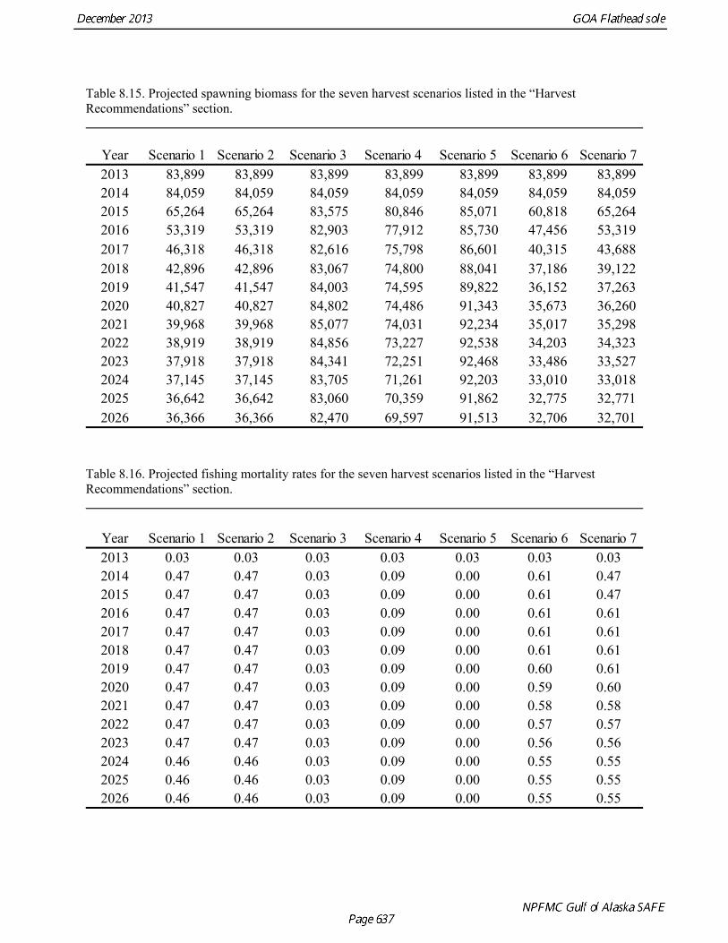
Table 8.15. Projected spawning biomass for the seven harvest scenarios listed in the “Harvest Recommendations” section.
Table 8.16. Projected fishing mortality rates for the seven harvest scenarios listed in the “Harvest Recommendations” section.
Year Scenario 1 Scenario 2 Scenario 3 Scenario 4 Scenario 5 Scenario 6 Scenario 72013 83,899 83,899 83,899 83,899 83,899 83,899 83,899 2014 84,059 84,059 84,059 84,059 84,059 84,059 84,059 2015 65,264 65,264 83,575 80,846 85,071 60,818 65,264 2016 53,319 53,319 82,903 77,912 85,730 47,456 53,319 2017 46,318 46,318 82,616 75,798 86,601 40,315 43,688 2018 42,896 42,896 83,067 74,800 88,041 37,186 39,122 2019 41,547 41,547 84,003 74,595 89,822 36,152 37,263 2020 40,827 40,827 84,802 74,486 91,343 35,673 36,260 2021 39,968 39,968 85,077 74,031 92,234 35,017 35,298 2022 38,919 38,919 84,856 73,227 92,538 34,203 34,323 2023 37,918 37,918 84,341 72,251 92,468 33,486 33,527 2024 37,145 37,145 83,705 71,261 92,203 33,010 33,018 2025 36,642 36,642 83,060 70,359 91,862 32,775 32,771 2026 36,366 36,366 82,470 69,597 91,513 32,706 32,701
Year Scenario 1 Scenario 2 Scenario 3 Scenario 4 Scenario 5 Scenario 6 Scenario 72013 0.03 0.03 0.03 0.03 0.03 0.03 0.032014 0.47 0.47 0.03 0.09 0.00 0.61 0.472015 0.47 0.47 0.03 0.09 0.00 0.61 0.472016 0.47 0.47 0.03 0.09 0.00 0.61 0.612017 0.47 0.47 0.03 0.09 0.00 0.61 0.612018 0.47 0.47 0.03 0.09 0.00 0.61 0.612019 0.47 0.47 0.03 0.09 0.00 0.60 0.612020 0.47 0.47 0.03 0.09 0.00 0.59 0.602021 0.47 0.47 0.03 0.09 0.00 0.58 0.582022 0.47 0.47 0.03 0.09 0.00 0.57 0.572023 0.47 0.47 0.03 0.09 0.00 0.56 0.562024 0.46 0.46 0.03 0.09 0.00 0.55 0.552025 0.46 0.46 0.03 0.09 0.00 0.55 0.552026 0.46 0.46 0.03 0.09 0.00 0.55 0.55

Table 8.17. Projected catches for the seven harvest scenarios listed in the “Harvest Recommendations” section.
Year Scenario 1 Scenario 2 Scenario 3 Scenario 4 Scenario 5 Scenario 6 Scenario 72013 2,861 2,861 2,861 2,861 2,861 2,861 2,861 2014 41,231 41,231 3,079 8,706 - 50,664 41,231 2015 31,114 31,114 3,081 8,381 - 35,371 31,114 2016 24,799 24,799 3,076 8,090 - 26,792 30,619 2017 21,001 21,001 3,071 7,844 - 22,148 24,331 2018 18,887 18,887 3,068 7,654 - 19,842 21,083 2019 17,821 17,821 3,072 7,525 - 18,682 19,502 2020 17,282 17,282 3,083 7,447 - 18,011 18,489 2021 16,886 16,886 3,098 7,400 - 17,436 17,671 2022 16,424 16,424 3,110 7,355 - 16,832 16,933 2023 15,932 15,932 3,111 7,294 - 16,298 16,333 2024 15,524 15,524 3,100 7,211 - 15,931 15,937 2025 15,240 15,240 3,078 7,115 - 15,739 15,735 2026 15,076 15,076 3,053 7,024 - 15,684 15,679

Table 8.18. Groundfish bycatch for GOA flathead sole target (in mt; AKFIN, as of November 4th, 2013)
2004 2005 2006 2007 2008 2009 2010 2011 2012 2013
Arrowtooth Flounder 1477 1756 839 723 801 1337 2650 842 815 1013
Atka Mackerel 8.5 1.8 17.4 35.6 2.7 17.1 10.5 10.3
Central GOA Skate, Big and Longnose
36.4
Flathead Sole 909 632 522 423 572 696 1242 371 419 470
GOA Deep Water Flatfish
0.1 2 2.7 4.5 17.9 45.4 18.8 11.6 1.8
GOA Dusky Rockfish 2.5 2.3
GOA Pelagic Shelf Rockfish
1.7 3.8 9.2 1.6
GOA Rex Sole 242 332 68.1 110 86.3 184 397 103 178 78.7
GOA Rougheye Rockfish
1.3 2.1 2.7 15.3 0.9 18.4 16.4
GOA Shallow Water Flatfish
40.2 2.5 28.7 26.2 41 94.9 122 78.4 150 48.2
GOA Shortraker Rockfish
0.7 7.1 2.6 1.3 1.7
GOA Shortraker/Rougheye Rockfish
2.3
GOA Skate, Big 21.1 30.3 22.7 65.6 53.2 112 30.8 57.4 14.6
GOA Skate, Longnose 10.9 11.5 13.2 10.8 23.7 30 16.6 59.7 7.9
GOA Skate, Other 52.5 37.8 11.8 19.8 4.7 12.6 18.9 12.5 17 7.9
GOA Thornyhead Rockfish
7.1 1.1 5.7 7.1 7.5 12.6 8.1
Northern Rockfish 4.5 11.4 0.4 1.1 6 7.1 1.6 13.3
Octopus
Other Rockfish 2.2 1.7 0.3
Other Species 59.5 73.9 16.1 34.7 13.9 9.2 21.5
Pacific Cod 194 153 38 131 125 279 297 93.7 134 102
Pacific Ocean Perch 16 8.5 4.1 10.8 1.8 1.8 74.3 1.9 2 19.2
Pollock 20.5 10.7 33.4 27 45.4 136 319 101 181 108
Sablefish 6.2 1.5 3.8 4.2 0.7 19 13.7 3.7 6.5 12.5
Sculpin 13.6 4.7 3
Shark 0.3
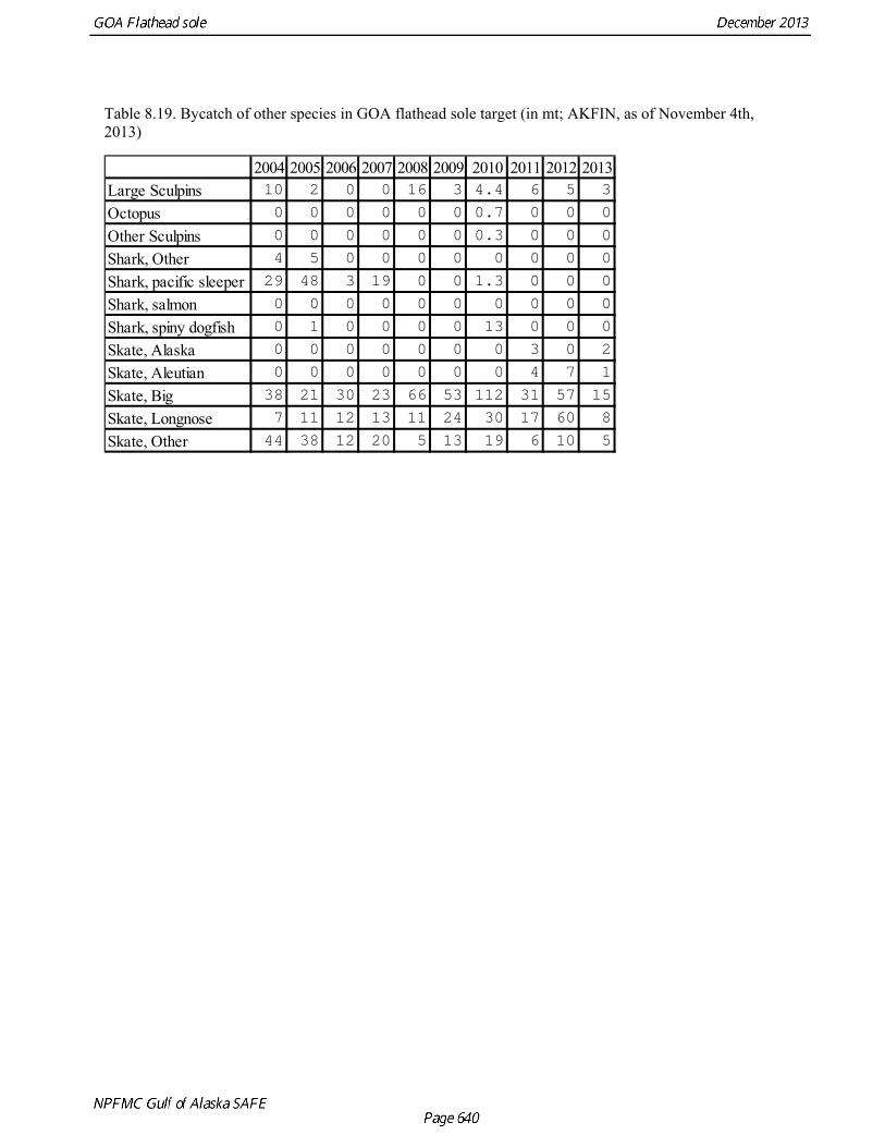
Table 8.19. Bycatch of other species in GOA flathead sole target (in mt; AKFIN, as of November 4th, 2013)
2004 2005 2006 2007 2008 2009 2010 2011 2012 2013
Large Sculpins 10 2 0 0 16 3 4.4 6 5 3
Octopus 0 0 0 0 0 0 0.7 0 0 0
Other Sculpins 0 0 0 0 0 0 0.3 0 0 0
Shark, Other 4 5 0 0 0 0 0 0 0 0
Shark, pacific sleeper 29 48 3 19 0 0 1.3 0 0 0
Shark, salmon 0 0 0 0 0 0 0 0 0 0
Shark, spiny dogfish 0 1 0 0 0 0 13 0 0 0
Skate, Alaska 0 0 0 0 0 0 0 3 0 2
Skate, Aleutian 0 0 0 0 0 0 0 4 7 1
Skate, Big 38 21 30 23 66 53 112 31 57 15
Skate, Longnose 7 11 12 13 11 24 30 17 60 8
Skate, Other 44 38 12 20 5 13 19 6 10 5

Table 8.20. Retained (R) and discarded (D) flathead sole in target fisheries (in mt; AKFIN, as of November 4th, 2013)
D R D R D R D R D R D R D R D R D R D R
Arrowtooth Flounder
85 702 94 1077 47 1200 114 1370 80 1113 3 1198 18 1080 36 1464 45 811 0 782
Atka Mackerel
0 0
Deep Water Flatfish
0 10 0 1 0 6 0 6 0 0
Flathead Sole
238 671 110 523 93 429 44 379 48 524 11 685 42 1194 13 358 7 412 10 461
Halibut 0 0 0 0 0 1 0 0 0 0
No retained catch
Other Species
1 11 0 0 0 1 0 0 0 1
Pacific Cod 29 38 5 14 76 104 29 214 9 313 13 95 10 33 5 150 3 158 3 183
Pollock - bottom
9 169 1 111 11 518 13 256 3 320 11 150 1 289 0 170 1 138 2 225
Pollock - midwater
21 60 2 54 0 59 1 56 1 80 0 54 0 61 0 43 2 48 1 72
Rex Sole 23 85 19 107 46 222 20 243 55 229 37 592 16 432 12 167 5 224 6 165
Rockfish 10 24 4 72 2 14 1 15 2 15 4 28 4 20 4 9 3 13 3 20
Sablefish 0 1 0 0 0 1 0 3 0 1 0 0 0 1 0 0 0 0
Shallow Water Flatfish
11 145 21 247 5 260 10 301 24 485 1 745 4 534 1 264 4 199 0 319
2010 2011 2012 20132004 2005 2006 2007 2008 2009

Table 8.21. Catch of non-target species in the flathead sole target fishery (in mt; AKFIN, as of November 4th, 2013)
2004 2005 2006 2007 2008 2009 2010 2011 2012 2013
Benthic urochordata 0.01 0 0 0 0 0 0 0.06 0.18 0
Bivalves 0.61 0.8 0.49 0.02 0.4 0.01 0.04 0.38 0 0.06
Brittle star unidentified 0 0 0 0 0 0 1.19 0.02 0 0
Capelin 0 0 0 0 0 0 0 0 0.01 0
Corals Bryozoans 0 0 0 0 0.15 0 0.02 0 0 0
Dark Rockfish 0 0 0 0 0 0.61 0 0 0 0
Eelpouts 0.12 0.46 0.12 0.11 0.01 0 12 2.09 0.04 0.11
Eulachon 0.05 20.4 1.62 0 0.21 0.07 0.28 0.13 0 0.39
Giant Grenadier 0 0 0 0 0 3.32 36 0 0 0
Greenlings 0.01 0 0 0 0 0 0.06 0.22 0 0
Grenadier 64.2 0.57 42.9 0 0 0 0 0.01 31.5 0
Gunnels 0 0 0.03 0 0.01 0 0 0 0 0
Hermit crab unidentified 0 0 0 0 0.21 0 0.01 0.05 0 0
Invertebrate unidentified 0.15 0 0.04 0 0 0 0 0.33 0 0
Misc crabs 0.18 0 0 0 0 0.01 0.09 0.02 0 0
Misc fish 1.11 0.46 0.41 0.15 5.66 3.91 17.3 2.28 5.05 4.42
Other osmerids 0 0 13.9 0 0 0 0 0.02 0 0
Pandalid shrimp 0.04 0.83 0.42 0 0.03 0.02 0.59 0.09 0.28 0.07
Polychaete unidentified 0 0 0 0 0 0 0 0.01 0 0
Scypho jellies 0.05 0 0.26 0 0 0.04 0.25 0 0 0
Sea anemone unidentified 0.21 0 0.02 0 0 0.06 0.69 0.46 0 0.03
Sea pens whips 0 0 0 0 0 0 0.04 0.03 0 0
Sea star 11.4 26.8 1.63 0.55 1.62 0.7 4.65 6.02 0.53 3.66
Snails 0.03 0.53 0.11 0 0.23 0.11 0.25 0.19 0.22 0.11
Sponge unidentified 0.98 0 0 0 0 0 0.09 0.01 0 0
Stichaeidae 0 1.65 0.5 0 0 0.02 0.16 0 0 0.02
urchins dollars cucumbers 0.01 0.12 0 0 0 0 0.08 0.1 0 0
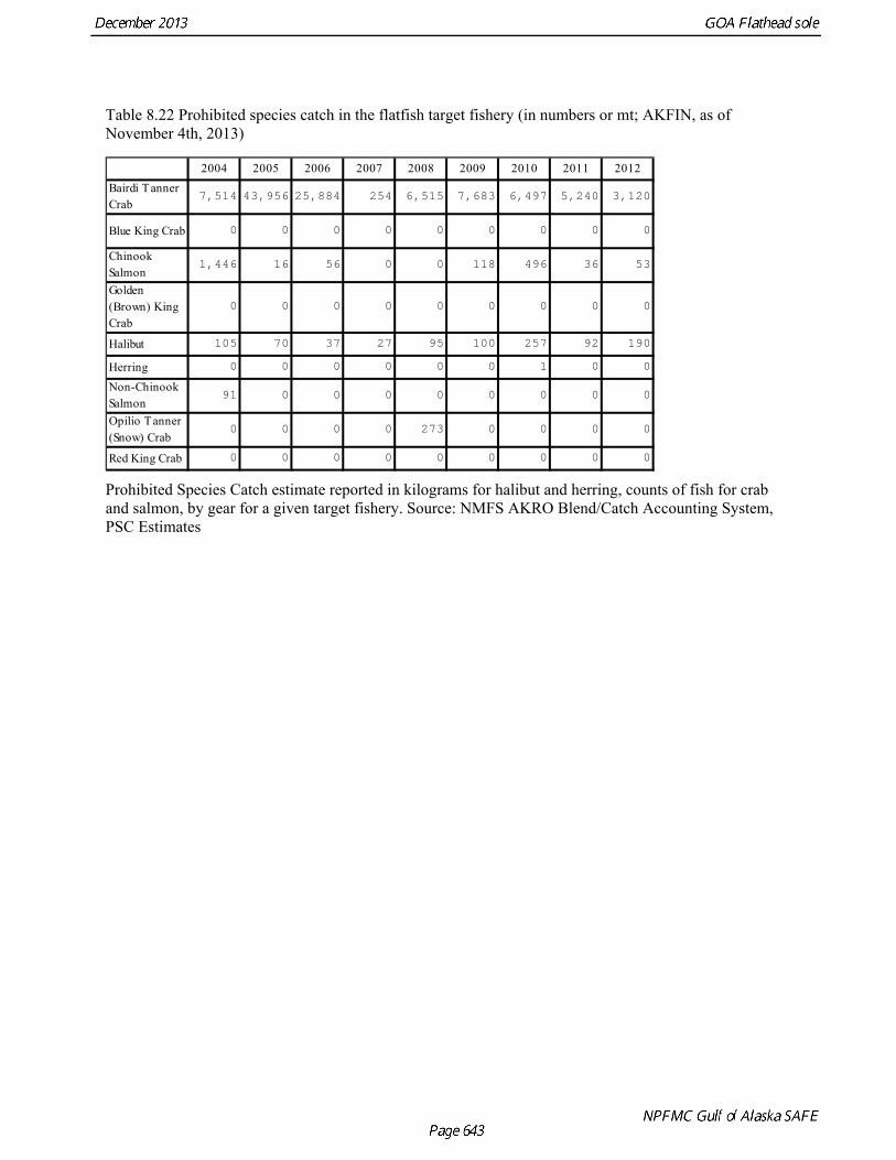
Table 8.22 Prohibited species catch in the flatfish target fishery (in numbers or mt; AKFIN, as of November 4th, 2013)
Prohibited Species Catch estimate reported in kilograms for halibut and herring, counts of fish for crab and salmon, by gear for a given target fishery. Source: NMFS AKRO Blend/Catch Accounting System, PSC Estimates
2004 2005 2006 2007 2008 2009 2010 2011 2012
Bairdi Tanner Crab
7,514 43,956 25,884 254 6,515 7,683 6,497 5,240 3,120
Blue King Crab 0 0 0 0 0 0 0 0 0
Chinook Salmon
1,446 16 56 0 0 118 496 36 53
Golden (Brown) King Crab
0 0 0 0 0 0 0 0 0
Halibut 105 70 37 27 95 100 257 92 190
Herring 0 0 0 0 0 0 1 0 0
Non-Chinook Salmon
91 0 0 0 0 0 0 0 0
Opilio Tanner (Snow) Crab
0 0 0 0 273 0 0 0 0
Red King Crab 0 0 0 0 0 0 0 0 0

FIGURES
Figure 8.1. Catch biomass in metric tons 1978-2013 (as of October 19, 2013).
Figure 8.2. Spatial distribution of fishery CPUE in 2009.
1980 1990 2000 2010
010
0020
0030
00
Year
Cat
ch (
mt)
1980 1990 2000 2010
010
0020
0030
00
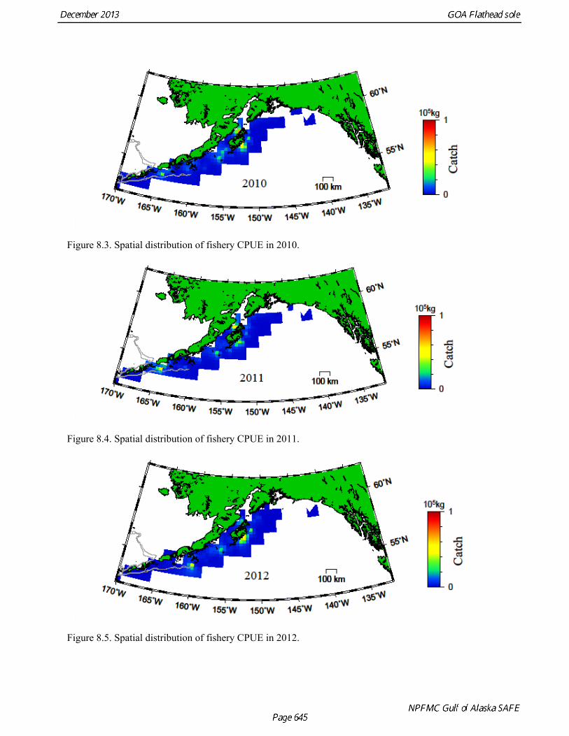
Figure 8.3. Spatial distribution of fishery CPUE in 2010.
Figure 8.4. Spatial distribution of fishery CPUE in 2011.
Figure 8.5. Spatial distribution of fishery CPUE in 2012.
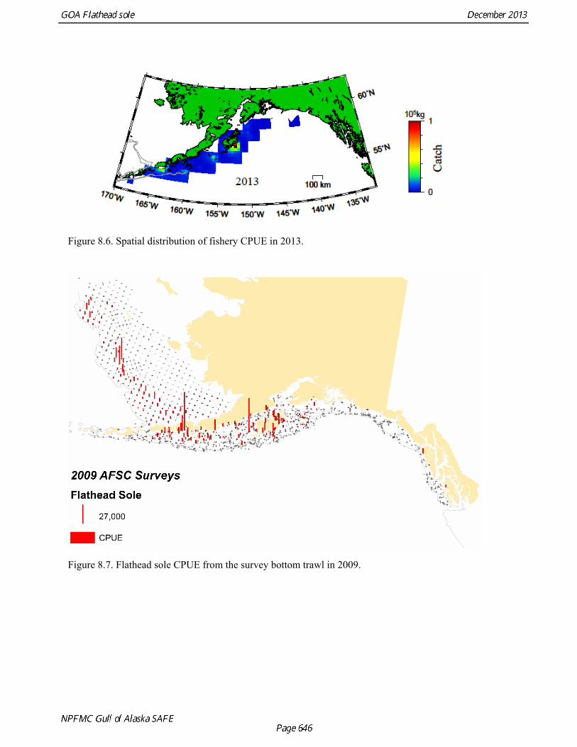
Figure 8.6. Spatial distribution of fishery CPUE in 2013.
Figure 8.7. Flathead sole CPUE from the survey bottom trawl in 2009.
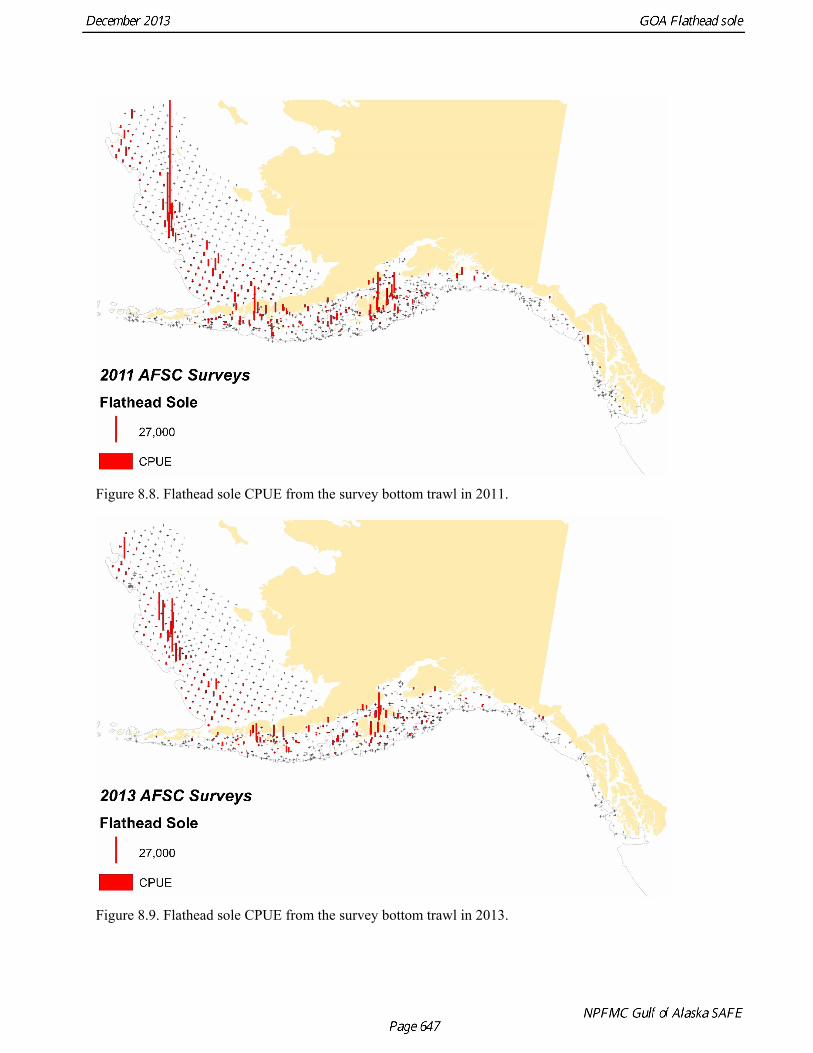
Figure 8.8. Flathead sole CPUE from the survey bottom trawl in 2011.
Figure 8.9. Flathead sole CPUE from the survey bottom trawl in 2013.

0 5 10 15 20 25 30
0.0
0.2
0.4
0.6
0.8
1.0
Age (yr)
Ma
turi
ty
Figure 8.10. Maturity-at-age relationship used for all model runs.
Figure 8.11. Survey biomass index (black dots), asymptotic 95% confidence intervals (vertical black lines), and estimated survey biomass for the four alternative models (solid lines).

Figure 8.12. Time series of spawning biomass and 95% asymptotic confidence intervals for the four alternative models.

Figure 8.13. Recruitment deviations for years 1978-2012 and 95% asymptotic confidence intervals for the four alternative models.
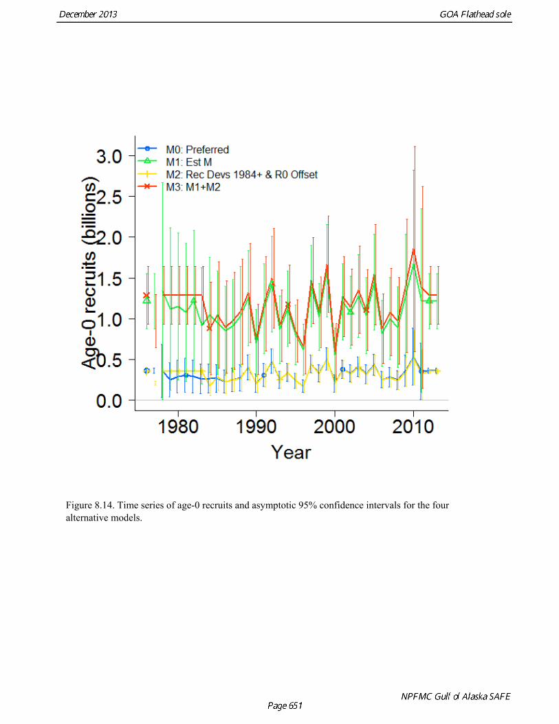
Figure 8.14. Time series of age-0 recruits and asymptotic 95% confidence intervals for the four alternative models.

Figure 8.15. Selectivity curves for the fishery (blue lines) and the survey (red lines), and for females (solid lines) and males (dashed lines) for Model 0 (fixed natural mortality) with the curve restricted such that selectivity reaches 1 by age 16.
Figure 8.16. Selectivity curves for the fishery (blue lines) and the survey (red lines), and for females (solid lines) and males (dashed lines) for Model 1 (estimated natural mortality). The selectivity parameters are unconstrained.

Figure 8.17. Selectivity curves for the fishery (blue lines) and the survey (red lines), and for females (solid lines) and males (dashed lines) for Model 2 (natural mortality is fixed and no early recruitment deviations are estimated). The selectivity curve was restricted such that selectivity reaches 1 by age 16.
Figure 8.18. Selectivity curves for the fishery (blue lines) and the survey (red lines), and for females (solid lines) and males (dashed lines) for Model 3 (natural mortality is estimated and early recruitment deviations are not estimated; there are no restrictions on selectivity parameters).

Figure 8.19. Selectivity curves for the fishery (blue lines) and the survey (red lines), and for females (solid lines) and males (dashed lines) for a model identical to Model 0 (fixed natural mortality), except without restrictions on the fishery selectivity curve.

Figure 8.20. Observed (grey shaded area, black lines) and expected (red lines) proportions-at-length, aggregated over years for the fishery and survey and for females (upper panel) and males (lower panel) for Model 0 (fixed natural mortality, estimated early recruitment deviations).
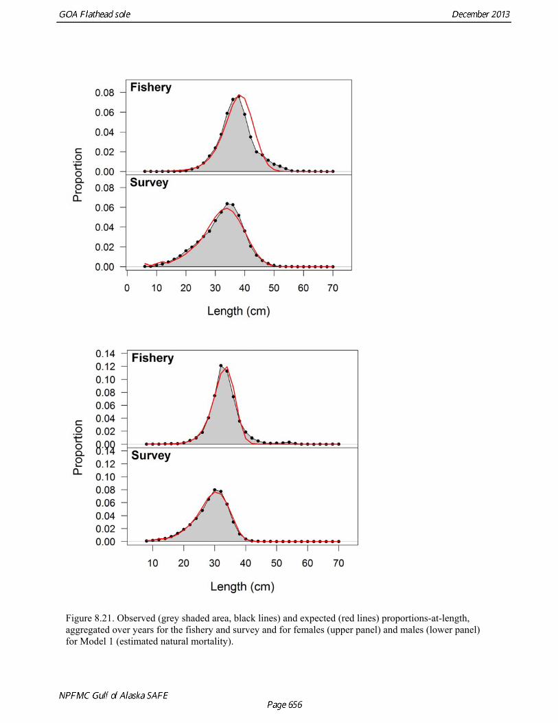
Figure 8.21. Observed (grey shaded area, black lines) and expected (red lines) proportions-at-length, aggregated over years for the fishery and survey and for females (upper panel) and males (lower panel) for Model 1 (estimated natural mortality).
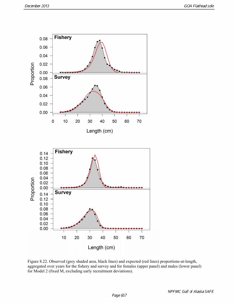
Figure 8.22. Observed (grey shaded area, black lines) and expected (red lines) proportions-at-length, aggregated over years for the fishery and survey and for females (upper panel) and males (lower panel) for Model 2 (fixed M, excluding early recruitment deviations).

Figure 8.23. Observed (grey shaded area, black lines) and expected (red lines) proportions-at-length, aggregated over years for the fishery and survey and for females (upper panel) and males (lower panel) for Model 3 (estimated natural mortality, excluded early recruitment deviations).
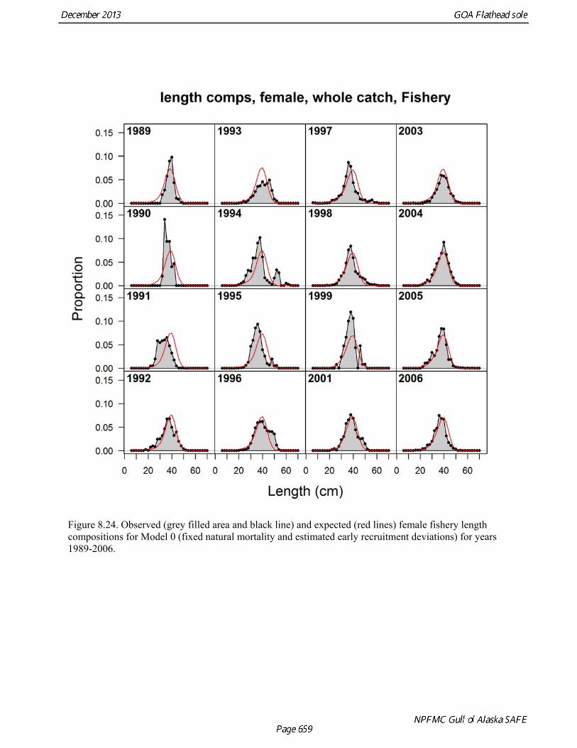
Figure 8.24. Observed (grey filled area and black line) and expected (red lines) female fishery length compositions for Model 0 (fixed natural mortality and estimated early recruitment deviations) for years 1989-2006.
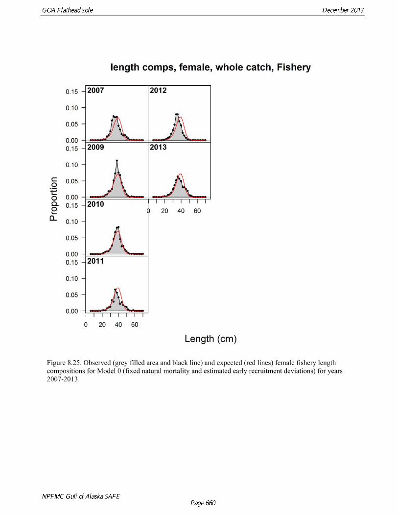
Figure 8.25. Observed (grey filled area and black line) and expected (red lines) female fishery length compositions for Model 0 (fixed natural mortality and estimated early recruitment deviations) for years 2007-2013.

Figure 8.26. Observed (grey filled area and black line) and expected (red lines) male fishery length compositions for Model 0 (fixed natural mortality and estimated early recruitment deviations) for years 1989-2006.
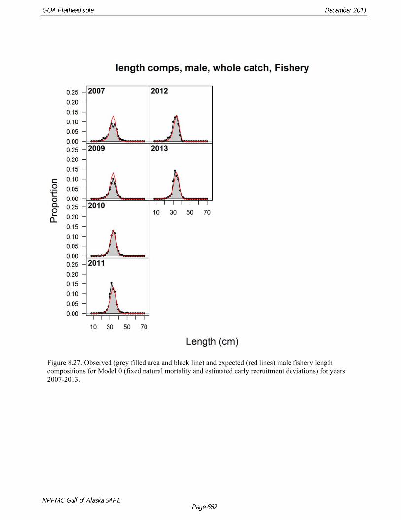
Figure 8.27. Observed (grey filled area and black line) and expected (red lines) male fishery length compositions for Model 0 (fixed natural mortality and estimated early recruitment deviations) for years 2007-2013.

Figure 8.28. Observed (grey filled area and black line) and expected (red lines) female survey length compositions for Model 0 (fixed natural mortality and estimated early recruitment deviations).

Figure 8.29. Observed (grey filled area and black line) and expected (red lines) male survey length compositions for Model 0 (fixed natural mortality and estimated early recruitment deviations).

Figure 8.30. Estimated length-at-age for females (red) and males (blue) and 95% intervals (dotted lines) for Model 0 (estimated natural mortality and early recruitment deviations).

Figure 8.31. Maturity-at-age, female and male weight-at-age at the beginning of the year for Model 0 (red dashed lines) and the previous assessment model. Maturity-at-age was fixed.
0 5 10 15 20 25 30
0.0
0.4
0.8
Age
Pro
po
rtio
n
0 5 10 15 20 25 30
0.0
0.4
0.8
Maturity at Age
2011 ModelSS3
0 5 10 15 20 25 30
0.0
0.2
0.4
0.6
0.8
Age
We
igh
t (kg
)
0 5 10 15 20 25 30
0.0
0.2
0.4
0.6
0.8
Female Beg of Year WtAtAge
2011 Model
SS3
0 5 10 15 20 25 30
0.0
0.2
0.4
0.6
0.8
Age
We
igh
t (kg
)
0 5 10 15 20 25 30
0.0
0.2
0.4
0.6
0.8
Male Beg of Year WtAtAge
2011 Model
SS3

Figure 8.32. Observed and expected female mean age-at-length with 90% intervals about observed age-at-length (left panels) and observed and expected standard deviation in age-at-length (right panels) for Model 0 (fixed natural mortality and estimated early recruitment deviations) for years 1990-1996.

Figure 8.33. Observed and expected female mean age-at-length with 90% intervals about observed age-at-length (left panels) and observed and expected standard deviation in age-at-length (right panels) for Model 0 (fixed natural mortality and estimated early recruitment deviations) for years 1999-2003.

Length (cm)
Figure 8.34. Observed and expected female mean age-at-length with 90% intervals about observed age-at-length (left panels) and observed and expected standard deviation in age-at-length (right panels) for Model 0 (fixed natural mortality and estimated early recruitment deviations) for years 2005-2011.

Figure 8.35. Observed and expected male mean age-at-length with 90% intervals about observed age-at-length (left panels) and observed and expected standard deviation in age-at-length (right panels) for Model 0 (fixed natural mortality and estimated early recruitment deviations) for years 1990-1996.

Figure 8.36. Observed and expected male mean age-at-length with 90% intervals about observed age-at-length (left panels) and observed and expected standard deviation in age-at-length (right panels) for Model 0 (fixed natural mortality and estimated early recruitment deviations) for years 1999-2003.

Length (cm)
Figure 8.37. Observed and expected male mean age-at-length with 90% intervals about observed age-at-length (left panels) and observed and expected standard deviation in age-at-length (right panels) for Model 0 (fixed natural mortality and estimated early recruitment deviations) for years 2005-2011.

Figure 8.38. Time series of spawning stock biomass (solid line) and asymptotic 95% confidence intervals (dotted lines) for Model 0.
Figure 8.39. Spawning stock biomass relative to B35% and fishing mortality (F) relative to F35% from 1978-2012 (solid black line), the OFL control rule (dotted red line), the maxABC control rule (solid red line), B35% (vertical grey line), and F35% (horizontal grey line) for Model 0 (fixed natural mortality and estimated early recruitment deviations).
Year
Spa
wni
ng s
tock
bio
mas
s0
4000
080
000
1200
00
1975 1985 1995 2005

Figure 8.40. Observed (grey filled area and black line) and expected (red lines) female fishery proportions-at-length for Model 1 (estimated natural mortality and early recruitment deviations) for years 1989-2006.
1989
0.00
0.05
0.10
0.15
length comps, female, whole catch, Fishery
Length (cm)
Pro
po
rtio
n
1990
0.00
0.05
0.10
0.15
1991
0.00
0.05
0.10
0.15
1992
0 20 40 60
0.00
0.05
0.10
0.15
1993
1994
1995
1996
0 20 40 60
1997
1998
1999
2001
0 20 40 60
2003
2004
2005
2006
0 20 40 60

Figure 8.41. Observed (grey filled area and black line) and expected (red lines) female fishery proportions-at-length for Model 1 (estimated natural mortality and early recruitment deviations) for years 2007-2013.
2007
0.00
0.05
0.10
0.15
length comps, female, whole catch, Fishery
Length (cm)
Pro
po
rtio
n
2009
0.00
0.05
0.10
0.15
2010
0.00
0.05
0.10
0.15
2011
0 20 40 60
0.00
0.05
0.10
0.15
2012
2013
0 20 40 60

Figure 8.42. Observed (grey filled area and black line) and expected (red lines) male fishery length compositions for Model 1 (estimated natural mortality and early recruitment deviations) for years 1989-2006.
1989
0.00
0.05
0.10
0.15
0.20
0.25
length comps, male, whole catch, Fishery
Length (cm)
Pro
po
rtio
n
1990
0.00
0.05
0.10
0.15
0.20
0.25
1991
0.00
0.05
0.10
0.15
0.20
0.25
1992
10 30 50 70
0.00
0.05
0.10
0.15
0.20
0.25
1993
1994
1995
1996
10 30 50 70
1997
1998
1999
2001
10 30 50 70
2003
2004
2005
2006
10 30 50 70

Figure 8.43. Observed (grey filled area and black line) and expected (red lines) male fishery length compositions for Model 1 (estimated natural mortality and early recruitment deviations) for years 2007-2013.
2007
0.00
0.05
0.10
0.15
0.20
0.25
length comps, male, whole catch, Fishery
Length (cm)
Pro
po
rtio
n
2009
0.00
0.05
0.10
0.15
0.20
0.25
2010
0.00
0.05
0.10
0.15
0.20
0.25
2011
10 30 50 70
0.00
0.05
0.10
0.15
0.20
0.25
2012
2013
10 30 50 70

Figure 8.44. Observed (grey filled area and black lines) and expected (red lines) female survey length compositions Model 1(estimated natural mortality and early recruitment deviations) for each year of length composition data included in the objective function.
1984
0.00
0.02
0.04
0.06
0.08
0.10
length comps, female, whole catch, Survey
Length (cm)
Pro
po
rtio
n
1987
0.00
0.02
0.04
0.06
0.08
0.10
1990
0.00
0.02
0.04
0.06
0.08
0.10
1993
0 20 40 60
0.00
0.02
0.04
0.06
0.08
0.10
1996
1999
2001
2003
0 20 40 60
2005
2007
2009
2011
0 20 40 60
2013
0 20 40 60

Figure 8.45. As for Figure 8.44, but for males: observed (grey filled area and black lines) and expected (red lines) male survey length compositions for Model 1 (estimated natural mortality and early recruitment deviations) for each year of length composition data included in the objective function.
1984
0.00
0.02
0.04
0.06
0.08
0.10
0.12
length comps, male, whole catch, Survey
Length (cm)
Pro
po
rtio
n
1987
0.00
0.02
0.04
0.06
0.08
0.10
0.12
1990
0.00
0.02
0.04
0.06
0.08
0.10
0.12
1993
10 30 50 70
0.00
0.02
0.04
0.06
0.08
0.10
0.12
1996
1999
2001
2003
10 30 50 70
2005
2007
2009
2011
10 30 50 70
2013
10 30 50 70

Figure 8.46. Estimated length-at-age for females (red) and males (blue) and 95% intervals (dotted lines) for Model 1 (estimated natural mortality and early recruitment deviations).

Figure 8.47. Observed and expected female mean age-at-length with 90% intervals about observed age-at-length (left panels) and observed and expected standard deviation in age-at-length (right panels) for Model 1 (estimated natural mortality and early recruitment deviations) for years 1990-1996.

Figure 8.48. Observed and expected female mean age-at-length with 90% intervals about observed age-at-length (left panels) and observed and expected standard deviation in age-at-length (right panels) for Model 1 (estimated natural mortality and early recruitment deviations) for years 1999-2003.
10 20 30 40 50
010
2030
Age
1999
Length (cm)
10 20 30 40 50
0.0
1.0
2.0
3.0
Std
ev (
Age
) (y
r) Observed (with 90% interval)Expected
10 20 30 40 50
010
2030
Age
2001
10 20 30 40 500
12
34
Std
ev (
Age
) (y
r)
10 20 30 40 50
010
2030
Age
2003
10 20 30 40 50
0.0
1.0
2.0
3.0
Std
ev (
Age
) (y
r)
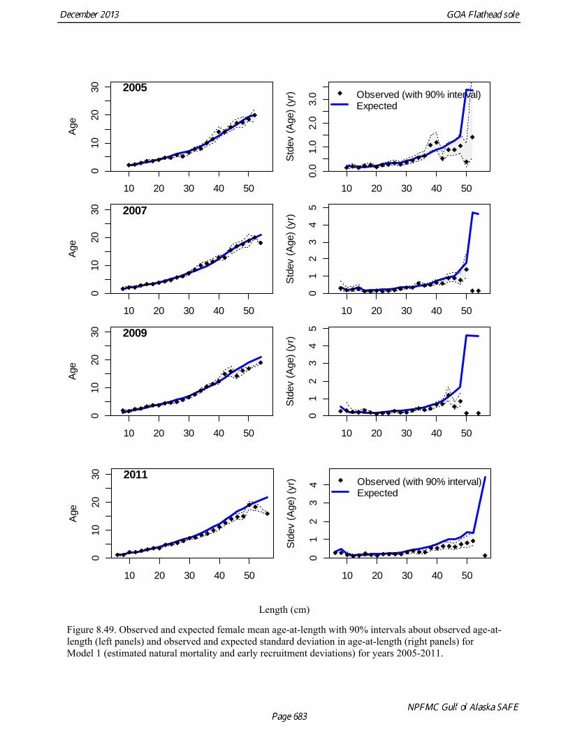
Length (cm)
Figure 8.49. Observed and expected female mean age-at-length with 90% intervals about observed age-at-length (left panels) and observed and expected standard deviation in age-at-length (right panels) for Model 1 (estimated natural mortality and early recruitment deviations) for years 2005-2011.
10 20 30 40 50
010
2030
Age
2005
10 20 30 40 50
0.0
1.0
2.0
3.0
Std
ev (
Age
) (y
r) Observed (with 90% interval)Expected
10 20 30 40 50
010
2030
Age
2007
10 20 30 40 500
12
34
5
Std
ev (
Age
) (y
r)
10 20 30 40 50
010
2030
Age
2009
10 20 30 40 50
01
23
45
Std
ev (
Age
) (y
r)
10 20 30 40 50
010
2030
Age
2011
10 20 30 40 50
01
23
4
Std
ev (
Age
) (y
r) Observed (with 90% interval)Expected

Figure 8.50. Observed and expected male mean age-at-length with 90% intervals about observed age-at-length (left panels) and observed and expected standard deviation in age-at-length (right panels) for Model 1 (estimated natural mortality and early recruitment deviations) for years 1990-1996.
10 20 30 40 50
010
2030
Age
1990
Length (cm)
10 20 30 40 50
01
23
45
Std
ev (
Age
) (y
r) Observed (with 90% interval)Expected
10 20 30 40 50
010
2030
Age
1993
10 20 30 40 500
12
34
Std
ev (
Age
) (y
r)
10 20 30 40 50
010
2030
Age
1996
10 20 30 40 50
0.0
1.0
2.0
Std
ev (
Age
) (y
r)

Figure 8.51. Observed and expected male mean age-at-length with 90% intervals about observed age-at-length (left panels) and observed and expected standard deviation in age-at-length (right panels) for Model 1 (estimated natural mortality and early recruitment deviations) for years 1999-2003.
10 20 30 40 50
010
2030
Age
1999
Length (cm)
10 20 30 40 50
0.0
1.0
2.0
Std
ev (
Age
) (y
r) Observed (with 90% interval)Expected
10 20 30 40 50
010
2030
Age
2001
10 20 30 40 500.
01.
02.
03.
0
Std
ev (
Age
) (y
r)
10 20 30 40 50
010
2030
Age
2003
10 20 30 40 50
0.0
1.0
2.0
3.0
Std
ev (
Age
) (y
r)

Length (cm)
Figure 8.52. Observed and expected male mean age-at-length with 90% intervals about observed age-at-length (left panels) and observed and expected standard deviation in age-at-length (right panels) for Model 1 (estimated natural mortality and early recruitment deviations) for years 2005-2011.
10 20 30 40 50
010
2030
Age
2005
10 20 30 40 50
01
23
45
Std
ev (
Age
) (y
r) Observed (with 90% interval)Expected
10 20 30 40 50
010
2030
Age
2007
10 20 30 40 500.
01.
02.
0
Std
ev (
Age
) (y
r)
10 20 30 40 50
010
2030
Age
2009
10 20 30 40 50
01
23
4
Std
ev (
Age
) (y
r)
10 20 30 40 50
010
2030
Age
2011
10 20 30 40 50
01
23
4
Std
ev (
Age
) (y
r) Observed (with 90% interval)Expected

Figure 8.53. Time series of spawning biomass in metric tons (mt) and 95% asymptotic confidence intervals for Model 1 (estimated natural mortality and early recruitment deviations).
Figure 8.54. Spawning stock biomass relative to B35% and fishing mortality (F) relative to F35% from 1978-2012 (solid black line), the OFL control rule (dotted red line), the maxABC control rule (solid red line), B35% (vertical grey line), and F35% (horizontal grey line) for Model 1 (estimated natural mortality and early recruitment deviations).
0 1 2 3 4
0.0
0.5
1.0
1.5
(Spawning Biomass)/B35%
F/F
35
%
1980 1990 2000 2010
02
00
00
60
00
01
00
00
0
Year
Sp
aw
nin
g b
iom
ass
(m
t)
-
-

Attachment 8A. September Safe document: an exploration of alternative models for GOA flathead sole
By Carey McGilliard
INTRODUCTION
The purpose of this document is to outline a proposed change from conducting assessments using the previously used flathead sole assessment model framework to conducting assessments using Stock Synthesis version 3.24o (SS3; Methot and Wetzel 2013).
Previous assessments were conducted using an ADMB-based age- and sex-structured population dynamics model with length-at-age, weight-at-length, maturity-at-age, and age-length transition matrices estimated outside of the model. The previous model estimated the log of mean recruitment, parameters for logistic age- and sex-specific selectivity curves for the fishery and survey, recruitment deviations, and yearly fishing mortality rates. The model included ages 3-20 and excluded data for fish below age 3 and 14 cm in length.
SS3 is a flexible assessment model framework that extends the capabilities of the 2011 flathead sole assessment model to address the concerns of the GOA Plan Team, the SSC, and previous flathead sole assessment authors, mentioned below. Although we do not expect that all concerns can addressed within the time-frame for the 2013 assessment cycle, this document outlines the work that was done to transition the flathead sole assessment from the previous assessment framework to SS3. In addition, proposed alternative models that address some previous concerns about the flathead sole assessment by using the extensive suite of modeling options available in SS3 are discussed.
DATA GAPS AND RESEARCH PRIORITIES FROM PREVIOUS ASSESSMENTS
Previous assessment authors suggest that the age-length transition matrices and other growth relationships used in the model are several years old and should be re-evaluated based on recent data. The previous authors recommend exploring estimation of growth relationships within the model. In addition, authors suggest that alternative selectivity functions be explored, including length-based fishery and survey selectivity, as well as functional forms other than the logistic curve.
One currently unfulfilled SSC request exists:
SSC request: The SSC requested that the next round of assessments consider the possible use of ADF&G bottom trawl survey data to expand the spatial and depth coverage.
The previous framework for conducting flathead sole assessments was unable to estimate growth or length-based selectivity, and accommodated only one survey. All of these concerns can be readily explored using SS3. Relative to the 2011 model, SS3 offers the following features:
(1) SS3 is used by many scientists worldwide, which provides an ad-hoc quality control system for
identifying bugs in the code. (2) A request from previous authors concerning the flathead sole assessments was that the age-length
transition matrices and other growth parameters be re-examined and potentially estimated within the model. The 2011 model had limited capability to do this, but such flexibility is included in the SS3 framework.

(3) Mean weight-at-age data can be included in the SS3 model and can be used as a likelihood component to help estimate growth. Since these data are available for GOA flathead sole, their use within the assessment model would be advantageous.
(4) SS3 has many options for specifying the functional form of selectivity curves and these could be used to explore length-based fishery and survey selectivity for flathead sole, which may be a more accurate reflection of the selection process than the age-based selectivity functions used in previous assessments.
(5) SS3 allows for specification of ageing error. Ageing error is ignored in the current model. (6) SS3 allows for multiple survey and fishing fleets to be included in the model. This feature would
be needed to explore the inclusion of the ADF&G bottom trawl survey in future assessments; the previous model accommodated only one fishery and one survey.
(7) SS3 accommodates age-composition data for ages 0-2. The previous assessment model omitted data for fish below age 3. Including data for ages 0-2 may inform recruitment estimates and age-based selectivity at young ages.
(8) SS3 allows for calculation of mid-year weight-at-age, which is an improvement over the 2011 model because it more accurately matches biological processes that occur during the year with respect to the timing of fishing. In previous models, exploitable biomass was calculated based on beginning-of-the-year weight-at-age, but fishing occurs over 7 months from January-November, and therefore using mid-year weight-at-age to calculate exploitable biomass may be more accurate.
(9) The previous assessment model assumed the stock was unfished prior to the model start year, but we know that fishing occurred before 1984. SS3 allows the user to estimate an initial fishing mortality rate to account for fishing prior to the availability of catch data.
(10) SS3 offers a “jitter” option, which allows for initial parameter values to be adjusted by a random deviate. Iteratively running the model with the “jitter” option turned on allows the user to start the model from a wide range of initial values so as to identify the best objective function value.
ANALYTIC APPROACH: TRANSITION OF 2011 MODEL INTO AN EQUIVALENT SS3 MODEL
Matching population dynamics between models
Mean recruitment
Several steps were taken to build an SS3 model with population dynamics that matched those of the 2011 model using deterministic models with no estimation of parameters and no recruitment deviations. First,
the relationship between the log of mean recruitment estimated in the 2011 model ( ) and the log of
R0 (unfished recruitment; ) that is estimated in SS3 was determined (Equation 1), where M is
natural mortality.
(1)
The estimated in the 2011 model refers to female mean recruitment of age 3 individuals,
while refers to total recruitment (males and females) of age 0 individuals in thousands;
both models assume a 1:1 sex ratio (but any sex ratio can be specified in SS3; a different sex ratio would change Equation 1). Using Equation 1, equivalent deterministic runs were
ln( )R
0ln( )R
0ln( ) ln(2R /1000) 3R M
ln( )R
0ln( )R

conducted, where both models were run with no recruitment deviations and no parameter estimation. Parameters were fixed at the maximum likelihood estimates (MLEs) from the 2011 model to ensure that both models had the same behavior in the absence of estimation. Equation 1 ensures that numbers at age 3 and above are the same in both models for an unfished population.
Selectivity
The 2011 model assumed sex-specific age-based logistic selectivity functions for fishery and survey selectivity. Although SS3 has logistic, sex-specific selectivity, it was found that the specification of male logistic age-based selectivity in SS3 was difficult to cast into a logistic shape. Sex-specific length-based logistic selectivity can be specified such that selectivity can be estimated for both sexes while retaining the logistic shape, or age-based double normal selectivity curves could be specified with a large value for the standard deviation of the descending limb such that asymptotic, logistic-like, sex-specific selectivity could be estimated. In the interest of matching the 2011 model as closely as possible, the age-based, sex-specific double normal selectivity curves without descending limbs were used for fishery and survey selectivity curves. The fishery selectivity curves were matched as closely as possible to the age-based logistic curves from the 2011 model for the purpose of comparing population dynamics between the models (Figure 8A.1). Figure 8A.1 shows that the double-normal selectivity curves can approximate the logistic curves from the 2011 model, but the shapes are slightly different and this results in small differences in population dynamics between the 2011 and SS3 models (Figure 8A.2). Figure 8A.2 shows that spawning stock biomass (SSB) is nearly, but not exactly the same between models in equivalent deterministic runs. Figure 8A.3 shows that survey biomass is also almost exactly the same between models in equivalent deterministic runs. The very small differences in spawning stock biomass in Figure 8A.2 can be explained by the differences in fishery selectivity curves shown in Figure 8A.1, as further equivalent deterministic runs (conducted for Dover sole) using selectivity curves that matched more exactly (but were still logistic for the 2011 model and double-normal for the SS3 model; Figure 8A.4) led to the same time series of SSB for both models (Figure 8A.5).

Stock-Recruitment
The 2011 model estimated recruits as median-unbiased recruitment deviations from their mean value. The SS3 model was configured similarly by specifying a Beverton-Holt stock-recruitment curve with a steepness of 1. SS3 estimates mean-unbiased recruitment deviations by specifying
and applying a bias adjustment factor. For the deterministic runs, was set to 1.0E-06, and
for runs when recruitment deviations were estimated, was set to 0.60. The 2011 model
estimated recruits (age 3) freely (i.e. no ) and this constitutes a difference between the models.
Growth
The 2011 model used empirical estimates of maturity-at-age sex-specific somatic weight-at-age. SS3 also can use similar empirically specified values for the calculation of spawning stock biomass and biomass-at-age (Figure 8A.6). A benefit of using the SS3 framework is the ability to specify and estimate growth parameters internally. When growth parameters are specified (instead of age-specific schedules), small differences arise between models because SS3 uses the beginning of the year weight-at-age to calculate SSB (like in the 2011 model), but uses mid-year weight-at-age to calculate exploitable and survey biomass (the 2011 model uses beginning-of-the-year weight-at-age for all calculations).
In addition, age-length transition matrices were specified directly in the 2011 model whereas in SS3 they are computed from specified von-Bertalanffy growth curve parameters and CVs in length-at-age. To match population dynamics between models, the CVs of the youngest and oldest age classes were estimated externally and specified within SS3. The resulting age-length transition matrices output from SS3 runs were examined to check that they closely matched those used in 2011. A request concerning the previous flathead sole assessments was that the age-length transition matrices and other growth parameters be re-examined and potentially estimated within the model. SS3 provides ample flexibility to explore growth relationships whereas this option was unavailable in the 2011 model.
Biomass
Differences in total biomass will occur between the models because SS3 includes ages 0-2. However, SSB and survey biomass were shown to be matched precisely between models when run deterministically when selectivity curves match between models and other parameters are fixed (Figure 8A.3 & Figure 8A.5).
Timing
Both the SS3 and 2011 model calculated spawning stock biomass, survey biomass, and recruitment at the beginning of the year. SS3 calculates exploitable biomass in the middle of the year, but a vector for weight-at-age was manually provided to SS3, which forced the model to use beginning-of-the year weight-at-age in the exploitable biomass calculation to match the 2011 model as closely as possible.
DATA USED IN SS3 AND THE 2011 MODEL
The same data used in the 2011 flathead sole assessment model (Stockhausen et al. 2011, page 757) were used in the SS3 model: survey biomass, survey age- and length-compositions (triennial for 1984-1999 and biennial for 2001-2011), fishery length-composition data (1985-2011), and catch history (1984-2011). An important difference between the 2011 model and SS3 is that the youngest age class in the 2011 model (age 3) represents only age 3 individuals, while
R R
R
R

SS3 population dynamics begin at age 0 and consider the lowest age and length bins of data to be the proportion of individuals ages 0-3 and lengths 0-the upper limit of the lowest length bin, respectively. Therefore, age- and length-composition data must include ages 0-2 and any lengths no matter how small in SS3, while the 2011 model omitted data on ages 0-2 (and excluded data on fish smaller than 18cm). That SS3 included data on ages 0-2 likely informs estimates of selectivity at the lowest ages and hence improves recruitment estimates (especially in the most recent years). Ignoring this difference between models will result in extreme differences between expected and observed age- and length-compositions for the youngest age and length bins when selectivity at these ages and lengths is greater than 0. An alternative solution to including additional data in SS3 model runs was to specify an additional selectivity-at-length curve as a knife-edge curve with selectivity equal to zero at lengths where fish are likely to be younger than age 3 (in SS3 it is possible to specify selectivity-at-age and at-length at the same time). This was a coarse solution, as fish at age 3 are a variety of lengths and it required internal specification of growth parameters, which meant that maturity-at-age and weight-at-age would not be an exact match between the 2011 model and the SS3 model. Therefore, the SS3 model was set up to match the 2011 model, but included data on proportions at ages 0-2. Likewise, proportions at lengths smaller than 14cm were included in the lowest (14-16cm) length bin.
In 2001, surveys covered a more restricted depth range than in other years and it is thought that the survey did not cover the range of flathead sole. This was handled in the 2011 model and in SS3 by inflating survey biomass estimate by assuming that the survey covered 90% of the stock’s range.
PARAMETER ESTIMATION IN SS3 AND THE 2011 MODEL
Parameters Estimated Inside the Assessment Model
SS3 and 2011 model runs were conducted with estimation of the log of mean recruitment, recruitment deviations, fishing mortality rates (using the same empirical growth vectors in both models), and selectivity parameters. Selectivity parameters for the fishery and survey were estimated; the location of peak selectivity and the width of the ascending limb of the selectivity curve were estimated in SS3 and the age at 50% selection as well as the slope of the logistic selectivity curves were estimated in the 2011 model.
Likelihood component for survey biomass index
Table 8A.2 lists the likelihood components used in SS3 and the 2011 model. The likelihood component for the survey biomass index and the data used to calculate the survey biomass likelihood component are the same for both models. The 2011 model and SS3 survey biomass values match almost exactly in a deterministic model with no estimation (Figure 8A.3).
Age- and length-composition likelihood components
The age- and length-composition likelihood components in SS3 are identical to those in the 2011 model. However, as noted above, the observations of survey proportions-at-age and proportions-at-length differ among models in that the data given to SS3 includes the data given to the 2011 model in addition to the proportions of age 0-2 fish and lengths below 14cm. Therefore, the values of these likelihood components cannot be compared directly between the 2011 model and SS3, but are expected to have

similar influences on model fits. The fits to age- and length-composition data are very similar among models (Figure 8A.12-Figure 8A.14). The addition of age 0-2 and small length data included in the SS3 model likely contribute to differences in numbers at age 3 and selectivity parameter estimates. There is no easy way to test the extent to which the additional data contributes to differences, as the 2011 model does not accept the additional data, while it is required for the SS3 model.
Recruitment likelihood components
Recruitment likelihood components differ slightly between models. The 2011 model does not include a CV for recruitment deviations. In SS3 and in the 2011 model, the “main period” recruitment deviations must sum to 0 and recruitment deviations for all years (1967-2011) were included in the main period. No early or late-period recruitment deviations were included in either model.
ANALYTIC APPROACH: PROPOSED ALTERNATIVE SS3 MODELS
The following models are proposed alternatives to the transitional SS3 model that was constructed to match the dynamics of the 2011 model:
M0: The transitional SS3 model described above (the SS3 model that best matches the dynamics of the 2011 model)
M1: Length-based, logistic, sex-specific fishery selectivity. The fishery data consist only of length compositions and therefore the model may be able to estimate length-based selectivity more effectively than age-based selectivity. Fishery selectivity may be more a process of length (e.g. due to the net’s mesh size) than age (where multiple ages of fish are the same length). SS3 is able to estimate length-based, sex-specific, logistic fishery selectivity, so there is no need to use a double-normal curve without a descending limb for this alternative.
M2: Estimate an initial equilibrium fishing mortality rate. The transitional SS3 model assumes that the stock was unfished prior to the model start year (1984) even though fishing occurred before 1984. In the transitional model, estimates of recruitment for years prior to 1984 were below average, which may be an artifact to account for fishing that occurred prior to 1984.
M3: Length-based, logistic, sex-specific selectivity for the fishery and the survey.
M4: A combination of M2, and M3, where an initial equilibrium fishing mortality rate is calculated, and both the fishery and survey selectivity selectivity are estimated using logistic, sex-specific, length-based functions.
In addition, models that estimated recruitment deviations for an early period (1967-1983, for which there are no data) separately from the main recruitment period were explored so that recruitment deviations from years with little information would not influence the estimates of recruitment deviations in the period over which more information is available by way of the constraint that deviations must sum to 0. These models did not lead to a better fit to the data.
FURTHER PROPOSED ALTERNATIVE MODELS
The SS3 model framework facilitates the potential for the following analyses to be conducted:
‐ Estimating growth parameters internally to re-evaluate the age-length transition matrices and other growth relationships with inclusion of the most recent data.

‐ Adding mean weight-at-age data to the assessment and estimating growth parameters internally. Data on mean weight-at-age are available, but are not currently being used in analyses of GOA flathead sole. Mean weight-at-age is expected to inform estimates of growth parameters.
‐ Estimating growth parameters and the age-length transition matrix outside of the model using data that includes the most recent years.
‐ Including ageing error in the model: the previous assessment models ignored ageing error. The CVs about the length-at-age relationship are quite large. This implies that there are some age 3 fish that are the same length as some age 20+ fish, which is likely untrue and could potentially be attributed to ageing error.
‐ Re-evaluating effective sample sizes for age- and length-composition data. There are abrupt year-to-year changes in age-compositions that occur in the observations that are likely due to observation error. Using high effective sample sizes may exclude some process errors which should be considered.
RESULTS: TRANSITION OF 2011 MODEL INTO AN EQUIVALENT SS3 MODEL
The 2011 and SS3 models each estimated a similar time series of numbers at age 3 (considered recruits in the 2011 model), but the SS3 model estimated fewer numbers at age 3 than the 2011 model early in the time series (Figure 8A.7). Numbers at age 3 in the last two years of the time series were the most different between the models. However, data available to estimate recruitment in these years was limited. SSB estimates were similar, but not the same in the two models. SS3 estimated smaller values for SSB than those estimated by the 2011 model in most years represented in the time series (except for the initial years; Figure 8A.8). The fishery and survey selectivity curves for both males and females were shifted slightly to the left by 0-2 ages and were slightly steeper in the SS3 model than in the 2011 model (Figure 8A.9 & Figure 8A.10). This may explain why SSB was slightly lower for the SS3 model than for 2011 model (Figure 8A.8): the 2011 model estimates that there are more fish out there that aren’t being caught in the fishery or the survey than in the SS3 model. Figure 8A.11 shows observed and predicted survey biomass for the 2011 and SS3 models. The negative log likelihoods for the survey biomass likelihood component indicate that the SS3 model fit to the survey biomass data (-lnL = -6.71) was better than the fit from the 2011 model (-lnL = +14.0). The predicted survey biomass from the SS3 model appeared to be a better fit to the data for surveys conducted from 1993 – 2001. In general, fits to age- and length-composition data were similar for both models (Figure 8A.12-Figure 8A.14).
Summary and discussion of differences between the SS3 Model and 2011 Model
The differences between the configurations of the 2011 model and the SS3 model are:
(1) Both models used asymptotic selectivity curves, but the SS3 selectivity curves were parameterized with a double-normal function with no descending limb (the standard deviation for the descending limb was set to a very high value), while the selectivity curves for the 2011 model were logistic. In addition, the 2011 model re-normalizes the selectivity curves such that the largest selectivity occurred at 1. The asymptotic double-normal can approximate the logistic curve, but varied slightly. SS3 does not have an option for normalizing the selectivity curves such that the greatest selectivity is always equal to 1, but the curve can be specified such that the peak value is at 1. In addition, selectivity below age 3 cannot be fixed at 0 unless using a cubic spline selectivity approach, which would add other difficulties to the assessment.

(2) SS3 population dynamics begin at age 0 and 2011 model dynamics begin at age 3. The SS3 model is given additional data, which consist of survey age-compositions for ages 0-2 and length-compositions for lengths 0-13cm.
RESULTS: PROPOSED ALTERNATIVE SS3 MODELS
Table 8A.3 shows the negative log likelihood components for each of the proposed alternative models (M0-M4). All alternative models (M1-M4) had lower negative log likelihoods than the transitional SS3 model (M0). Negative log likelihoods were best for alternative models M3 and M4 (the two proposed alternative models that estimated length-based, logistic, sex-specific fishery and survey selectivity). Models M3 and M4 had better fits to the length-composition likelihood component than the other models, while models M0 and M2 had the best fits to the survey biomass likelihood component (Table 8A.3). However, fits to the survey biomass data were similar among alternative models (Figure 8A.18). Model M3 and M4 led to the highest estimated number of recruits and SSB (Figure 8A.15 & Figure 8A.17). Estimated recruitment deviations were similar among models (Figure 8A.16).
Proposed alternative model M4, which estimated an initial equilibrium fishing mortality rate and length-based, logistic, sex-specific fishery and survey selectivity, led to the best negative log likelihood of all of the SS3 models and a comparison to the 2011 model, including fits to the age- and length-composition data are shown in Figure 8A.23-Figure 8A.28. Model M4 and the 2011 model led to very similar estimates of SSB (Figure 8A.24). Fits to age- and length-composition data were similar for the two models (Figure 8A.26-Figure 8A.28).
LITERATURE CITED
Methot, R. D. and C. R. Wetzel. 2013. Stock synthesis: A biological and statistical framework for fish stock assessment and fishery management. Fisheries Research 142:86-99.
Stockhausen, W.T., M.E. Wilkins and M.H. Martin. 2011. 8. Gulf of Alaska Flathead Sole. In Stock Assessment and Fishery Evaluation Report for the Groundfish Resources of the Gulf of Alaska. pp. 753-820. North Pacific Fishery Management Council, P.O. Box 103136, Anchorage AK 99510.

TABLES
Table 8A.1. Symbols used in this document.
Symbol Meaning
x sex
a age
f fleet (fishery or survey)
t time
Selectivity for fleet f, sex x, and age a
Nt,x,a Numbers at age a, time t, and sex s
wa Weight at age a
Zt,x,a Total mortality at age a, sex s, and time t
timing The timing of the survey during the year
It,f Observed survey biomass at time t for fleet f
SBt,f Predicted survey biomass at time t for fleet f
CVt,f CV of observed survey biomass at time t for fleet f
Number of age-composition observations at time t for sex x and fleet f
Observed proportion at age a, time t, fleet f, and sex x
Predicted proportion at age a, time t, fleet f, and sex x
Number of length-composition observations at time t for sex x and fleet f
Observed proportion at length l, time t, fleet f, and sex x
Predicted proportion at length l, time t, fleet f, and sex x
Estimated mean recruitment in year t
Recruitment CV (specified in SS3 only)
Bias adjustment factor at time t (specified in SS3 only)
Observed catch at time t
Predicted catch at time t
Standard error of catch at time t for fleet f (specified for SS3 only)
, ,f x aS
, ,t x fn
, , ,t x f ap
, , ,ˆ t x f ap
2, , ,t x fn
, , ,t x f lp
, , ,ˆ t x f lp
tR
R
tb
Cobst
Ct
,t f

Table 8A.2. Likelihood components used in the 2011 and SS3 models. Numbers in the component column are likelihood component weightings for: (SS3, 2011 Model).
Component SS3 2011 Model
Survey biomass equation
Survey biomass likelihood (1,1)
As for SS3
Age composition
(1, 1) As for SS3
Length Composition
(1,1) As for SS3
Main period recruits
(1,1) (sum to 0
constraint)
(sum to 0 constraint)
Catch
(30,30)
,( )t fSB, , , , , ,exp( timing( ))f x a t x a a t x a
x a
S N w Z , , , ,f x a t x a ax a
S N w
2, ,
2 ,
(ln(I ) ln( ))
2 ln( 1)t f t f
t survey f t f
SB
CV
, , ,, , , , ,
, , ,
lnˆ
t x f at x f t x f a
t x a t x f a
pn p
p
, , ,2, , , , , ,l
, , ,
lnˆ
t x f lt x f t x f
t x l t x f l
pn p
p
220112
21967
1ln( )
2t
t Rt R
Rb
2011
2
1967t
t
R
2
2,
ˆ(ln(C ) ln(C ))
2
obst t
t t f
2ˆ(ln(C ) ln(C ))obst t
t

Table 8A.3. Components of the negative log(likelihood) for each alternative proposed SS3 model. M0-M4 are the alternative model descriptors, which are described in full in the section “Analytic Approach: Proposed Alternative SS3 Models” on page 6. The “Total” likelihoods marked “but add’l component” include an additional likelihood component for initial equilibrium catch and therefore the likelihoods cannot be compared directly to those alternative models where a component for initial equilibrium catch was not estimated. However, the contribution of the initial equilibrium catch likelihood component to the total negative log(likelihood) is very small in each case.
Likelihood componentM0: Base
Case M1 M2 M3 M4
Total (not always comparable to the transitional model) 667.419 652.857
663.375 (but add'l component) 641.471
637.855 (but add'l
component)
Initial Equilibrium Catch NA 0.000951959 0.000767171
Survey Biomass -6.70951 -5.33251 -6.72469 -4.74592 -4.5957
Length Composition 519.345 496.413 516.659 486.471 484.249
Age Composition 160.548 167.396 159.916 166.139 165.535
Recruitment -6.01594 -5.77063 -6.72534 -6.39456 -7.33513

FIGURES
Figure 8A.1.SS3 double-normal selectivity curves matched as closely as possible to the 2011 model’s logistic fishery selectivity curves (the standard deviation of the descending limb of the selectivity curves was fixed at a large value to create an asymptotic curve).
0.0
0.2
0.4
0.6
0.8
1.0
0 5 10 15 20
Age
Pro
port
ion
Fishery Selectivity
2011 Model, females
SS3, females
2011 Model, males
SS3, males

Figure 8A.2.Spawning stock biomass for a deterministic run of the 2011 and SS3 models with parameters in both models fixed at the MLEs for the 2011 model with flathead sole catch history and no recruitment deviations. Fishery selectivity curves for the models were forced to match as closely as possible (Figure 8A.1).

Figure 8A.3. Survey biomass for a deterministic run of the 2011 and SS3 models with parameters in both models fixed at the MLEs for the 2011 model with flathead sole catch history, no recruitment deviations, and no estimation. Fishery selectivity curves for the models were forced to match as closely as possible (Figure 8A.1).
1985 1990 1995 2000 2005 2010
05
01
00
15
02
00
25
03
00
35
0
Year
Bio
ma
ss (
1,0
00
's m
t)
1985 1990 1995 2000 2005 2010
05
01
00
15
02
00
25
03
00
35
0
Predicted Survey Biomass, 2011 Model
Predicted Survey Biomass, SS3 Model

Figure 8A.4. Fishery selectivity used in deterministic runs (the same as the final estimate for fishery selectivity in the 2011 model). The SS3 selectivity curves pictured were created using a double-normal selectivity curve with no descending limb; the 2011 model selectivity curves are logistic.
0.0
0.2
0.4
0.6
0.8
1.0
0 10 20 30 40
Age
Pro
port
ion
2011 Model, females
2011 Model, males
SS3, females
SS3, males

Figure 8A.5. Spawning stock biomass for a deterministic run of the 2011 and SS3 models with parameters fixed at the MLEs for the 2011 Dover sole model with Dover sole catch history and no recruitment deviations. Fishery selectivity curves for the models were forced to match as closely as possible (Figure 8A.4).

Figure 8A.6. Maturity-at-age and weight-at-age for the 2011 model and an equivalent SS3 model.
0 5 10 15 20
0.0
0.2
0.4
0.6
0.8
1.0
Age
Pro
port
ion
0 5 10 15 20
0.0
0.2
0.4
0.6
0.8
1.0
Maturity at Age
2011 ModelSS3
0 5 10 15 20
0.0
0.2
0.4
0.6
0.8
Age
Wei
ght
(kg)
0 5 10 15 20
0.0
0.2
0.4
0.6
0.8
Female Beg of Year WtAtAge
2011 ModelSS3
0 5 10 15 20
0.0
0.2
0.4
0.6
0.8
Age
Wei
ght
(kg)
0 5 10 15 20
0.0
0.2
0.4
0.6
0.8
Male Beg of Year WtAtAge
2011 ModelSS3

Figure 8A.7. Numbers at age 3 for the 2011 model (black line) and an equivalent SS3 run (blue line). Both models estimate the log of mean recruitment, recruitment deviations for 1967-2011, fishing mortality rates, and asymptotic selectivity parameters (logistic for the 2011 model and double-normal for SS3). Survey data for ages 0-2 and lengths 0-14cm are included in the SS3 model, but not the 2011 model.
Year
Nu
mb
ers
at A
ge
3 (
in m
illio
ns)
01
00
20
03
00
40
0
1980 1985 1990 1995 2000 2005 2010
2011 Model
SS3
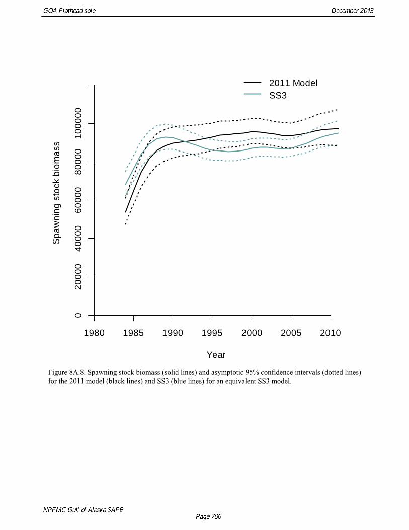
Figure 8A.8. Spawning stock biomass (solid lines) and asymptotic 95% confidence intervals (dotted lines) for the 2011 model (black lines) and SS3 (blue lines) for an equivalent SS3 model.
Year
Sp
aw
nin
g s
tock
bio
ma
ss
02
00
00
40
00
06
00
00
80
00
01
00
00
0
1980 1985 1990 1995 2000 2005 2010
2011 ModelSS3
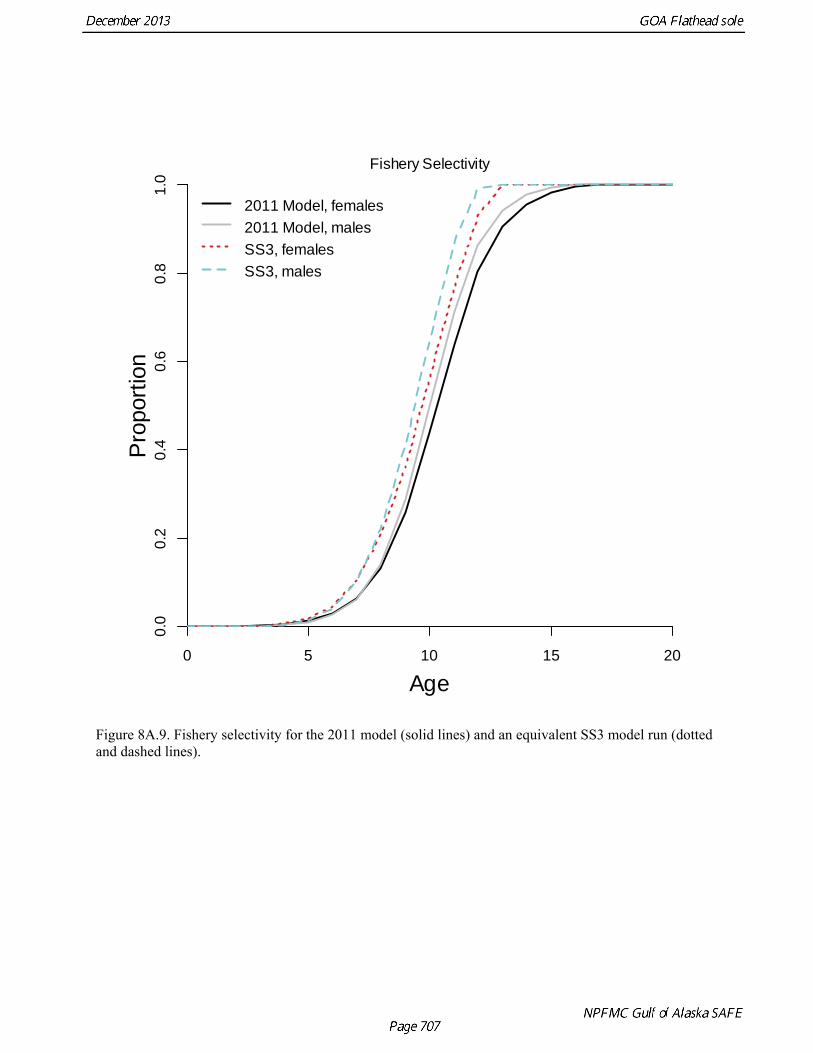
Figure 8A.9. Fishery selectivity for the 2011 model (solid lines) and an equivalent SS3 model run (dotted and dashed lines).
0.0
0.2
0.4
0.6
0.8
1.0
0 5 10 15 20
Age
Pro
port
ion
Fishery Selectivity
2011 Model, females
2011 Model, males
SS3, females
SS3, males
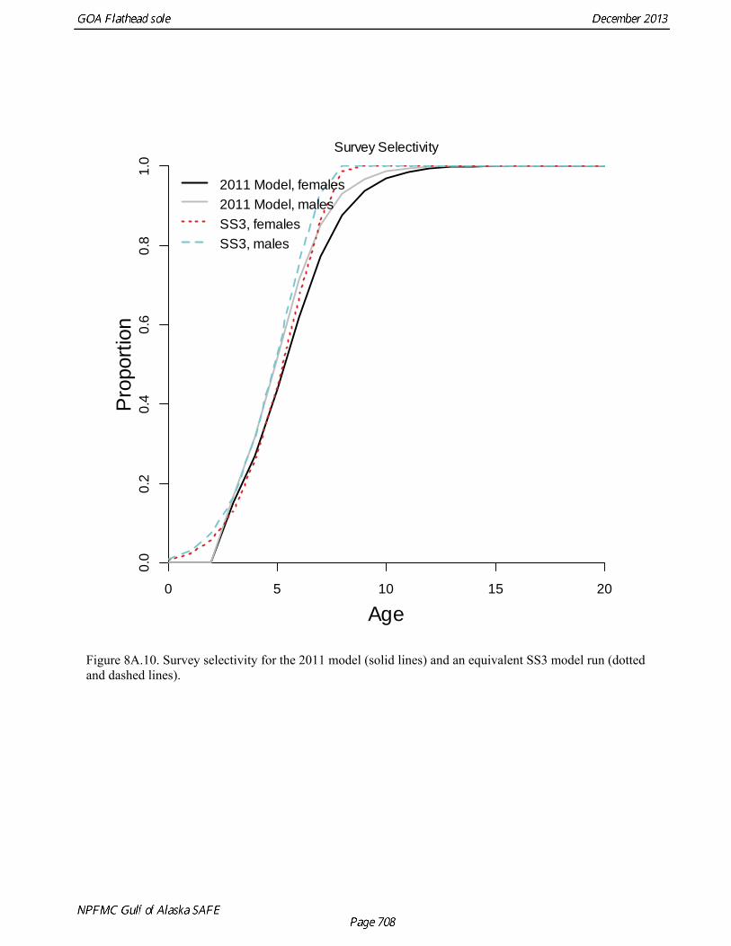
Figure 8A.10. Survey selectivity for the 2011 model (solid lines) and an equivalent SS3 model run (dotted and dashed lines).
0.0
0.2
0.4
0.6
0.8
1.0
0 5 10 15 20
Age
Pro
port
ion
Survey Selectivity
2011 Model, females
2011 Model, males
SS3, females
SS3, males

Figure 8A.11. Observed survey biomass (black dots) with 95% asymptotic confidence intervals (vertical black lines) and predicted survey biomass from the 2011 model (black line) and an equivalent SS3 model (blue line).
1985 1990 1995 2000 2005 2010
05
01
00
15
02
00
25
03
00
35
0
Year
Bio
ma
ss (
1,0
00
's m
t)
1985 1990 1995 2000 2005 2010
05
01
00
15
02
00
25
03
00
35
0
Predicted Survey Biomass, 2011 Model
Predicted Survey Biomass, SS3 Model
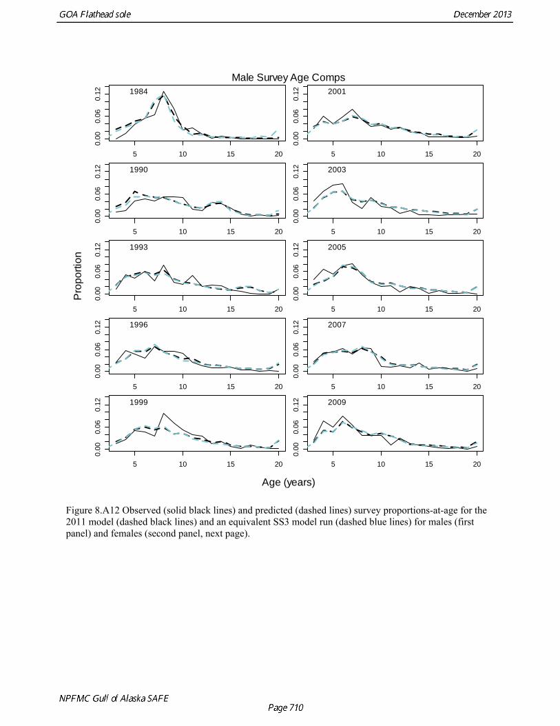
Figure 8.A12 Observed (solid black lines) and predicted (dashed lines) survey proportions-at-age for the 2011 model (dashed black lines) and an equivalent SS3 model run (dashed blue lines) for males (first panel) and females (second panel, next page).
5 10 15 20
0.00
0.06
0.12 1984
5 10 15 20
0.00
0.06
0.12 1990
5 10 15 20
0.00
0.06
0.12 1993
5 10 15 20
0.00
0.06
0.12 1996
5 10 15 20
0.00
0.06
0.12 1999
5 10 15 20
0.00
0.06
0.12 2001
5 10 15 20
0.00
0.06
0.12 2003
5 10 15 20
0.00
0.06
0.12 2005
5 10 15 20
0.00
0.06
0.12 2007
5 10 15 20
0.00
0.06
0.12 2009
Age (years)
Pro
po
rtio
nMale Survey Age Comps

Figure 8A.12, continued.
5 10 15 20
0.00
0.06
0.12 1984
5 10 15 20
0.00
0.06
0.12 1990
5 10 15 20
0.00
0.06
0.12 1993
5 10 15 20
0.00
0.06
0.12 1996
5 10 15 20
0.00
0.06
0.12 1999
5 10 15 20
0.00
0.06
0.12 2001
5 10 15 20
0.00
0.06
0.12 2003
5 10 15 20
0.00
0.06
0.12 2005
5 10 15 20
0.00
0.06
0.12 2007
5 10 15 20
0.00
0.06
0.12 2009
Age (years)
Pro
po
rtio
nFemale Survey Age Comps

Figure 8A.13. (1 of 6) Observed (solid black lines) and predicted (dashed lines) fishery proportions-at-length for the 2011 model (dashed black lines) and an equivalent SS3 model run (dashed blue lines) for females (first set of panels) and males (second set of panels).
20 30 40 50
0.00
0.15
1985
20 30 40 50
0.00
0.15
1986
20 30 40 50
0.00
0.15
1987
20 30 40 50
0.00
0.15
1988
20 30 40 50
0.00
0.15
1989
20 30 40 50
0.00
0.15
1990
20 30 40 50
0.00
0.15
1991
20 30 40 50
0.00
0.15
1992
20 30 40 50
0.00
0.15
1993
20 30 40 50
0.00
0.15
1994
20 30 40 50
0.00
0.15
1995
20 30 40 50
0.00
0.15
1996
Length (cm)
Pro
po
rtio
nFemale Fishery Size Comps

Figure 8A.13. (2 of 6)
20 30 40 50
0.00
0.15
1997
20 30 40 50
0.00
0.15
1998
20 30 40 50
0.00
0.15
1999
20 30 40 50
0.00
0.15
2000
20 30 40 50
0.00
0.15
2001
20 30 40 50
0.00
0.15
2002
20 30 40 50
0.00
0.15
2003
20 30 40 50
0.00
0.15
2004
20 30 40 50
0.00
0.15
2005
20 30 40 50
0.00
0.15
2006
20 30 40 50
0.00
0.15
2007
20 30 40 50
0.00
0.15
2008
Length (cm)
Pro
po
rtio
nFemale Fishery Size Comps
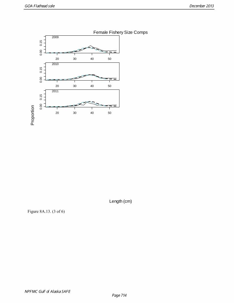
Figure 8A.13. (3 of 6)
20 30 40 50
0.00
0.15
2009
20 30 40 50
0.00
0.15
2010
20 30 40 50
0.00
0.15
2011
Length (cm)
Pro
po
rtio
nFemale Fishery Size Comps

Figure 8A.13. (4 of 6)
20 30 40 50
0.00
0.15
1985
20 30 40 50
0.00
0.15
1986
20 30 40 50
0.00
0.15
1987
20 30 40 50
0.00
0.15
1988
20 30 40 50
0.00
0.15
1989
20 30 40 50
0.00
0.15
1990
20 30 40 50
0.00
0.15
1991
20 30 40 50
0.00
0.15
1992
20 30 40 50
0.00
0.15
1993
20 30 40 50
0.00
0.15
1994
20 30 40 50
0.00
0.15
1995
20 30 40 50
0.00
0.15
1996
Length (cm)
Pro
po
rtio
nMale Fishery Size Comps

Figure 8A.13. (5 of 6)
20 30 40 50
0.00
0.15
1997
20 30 40 50
0.00
0.15
1998
20 30 40 50
0.00
0.15
1999
20 30 40 50
0.00
0.15
2000
20 30 40 50
0.00
0.15
2001
20 30 40 50
0.00
0.15
2002
20 30 40 50
0.00
0.15
2003
20 30 40 50
0.00
0.15
2004
20 30 40 50
0.00
0.15
2005
20 30 40 50
0.00
0.15
2006
20 30 40 50
0.00
0.15
2007
20 30 40 50
0.00
0.15
2008
Length (cm)
Pro
po
rtio
nMale Fishery Size Comps

Figure 8A.13 (6 of 6).
20 30 40 50
0.00
0.15
2009
20 30 40 50
0.00
0.15
2010
20 30 40 50
0.00
0.15
2011
Length (cm)
Pro
po
rtio
nMale Fishery Size Comps
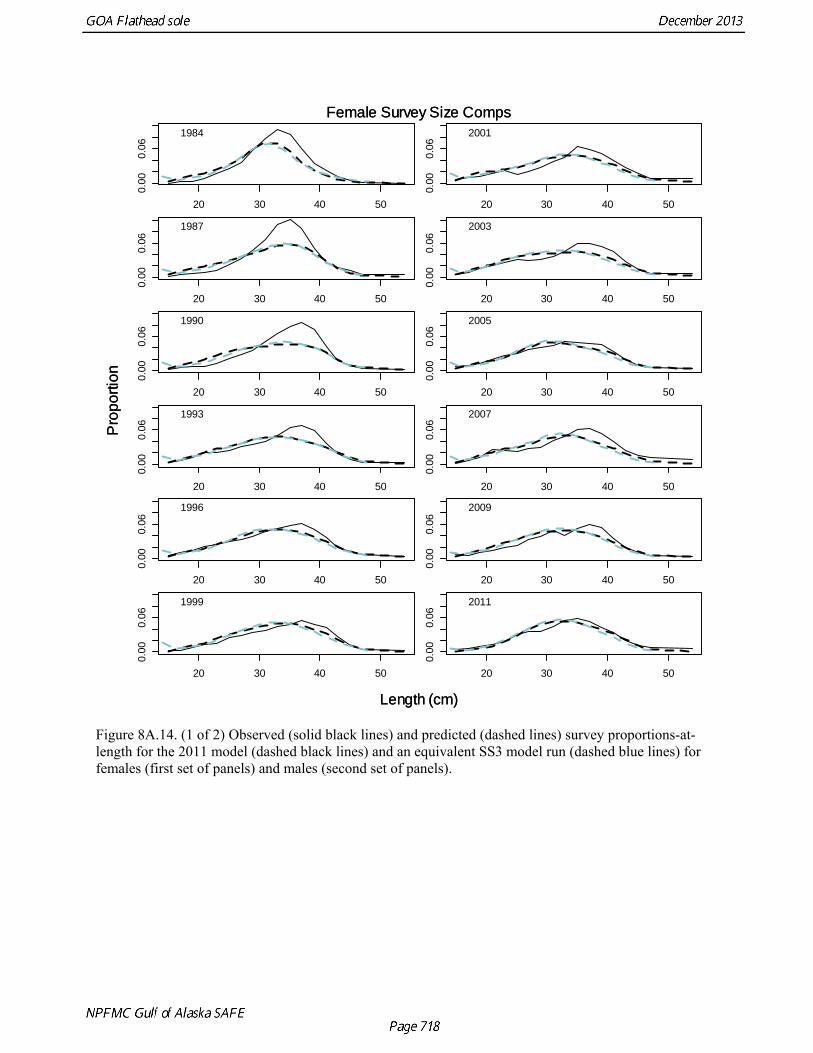
Figure 8A.14. (1 of 2) Observed (solid black lines) and predicted (dashed lines) survey proportions-at-length for the 2011 model (dashed black lines) and an equivalent SS3 model run (dashed blue lines) for females (first set of panels) and males (second set of panels).
20 30 40 50
0.00
0.06
1984
20 30 40 50
0.00
0.06
1987
20 30 40 50
0.00
0.06
1990
20 30 40 50
0.00
0.06
1993
20 30 40 50
0.00
0.06
1996
20 30 40 50
0.00
0.06
1999
20 30 40 50
0.00
0.06
2001
20 30 40 50
0.00
0.06
2003
20 30 40 50
0.00
0.06
2005
20 30 40 50
0.00
0.06
2007
20 30 40 50
0.00
0.06
2009
20 30 40 50
0.00
0.06
2011
Length (cm)
Pro
po
rtio
nFemale Survey Size Comps
Length (cm)
Pro
po
rtio
nFemale Survey Size Comps

Figure 8A.14. (2 of 2)
20 30 40 50
0.00
0.06
1984
20 30 40 50
0.00
0.06
1987
20 30 40 50
0.00
0.06
1990
20 30 40 50
0.00
0.06
1993
20 30 40 50
0.00
0.06
1996
20 30 40 50
0.00
0.06
1999
20 30 40 50
0.00
0.06
2001
20 30 40 50
0.00
0.06
2003
20 30 40 50
0.00
0.06
2005
20 30 40 50
0.00
0.06
2007
20 30 40 50
0.00
0.06
2009
20 30 40 50
0.00
0.06
2011
Length (cm)
Pro
po
rtio
nMale Survey Size Comps
Length (cm)
Pro
po
rtio
nMale Survey Size Comps

Figure 8A.15. Age 0 recruits for each alternative SS3 model. M0 is the transitional SS3 model that best matches the 2011 model. The leftmost group of vertical lines shows the log of mean recruitment.
Year
Ag
e-0
re
cru
its (
mill
ion
s)
M0M1M2M3M4
1985 1990 1995 2000 2005 2010
0
100
200
300
400
500
600

Figure 8A.16. Estimated recruitment deviations and 95% asymptotic confidence intervals for each alternative SS3 model. M0 is the transitional SS3 model that best matches the 2011 model.
1970 1980 1990 2000 2010
-2
-1
0
1
2
Year
Re
cru
itme
nt d
evi
atio
ns
M0M1M2M3M4
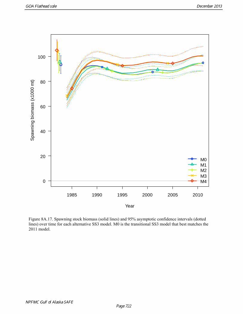
Figure 8A.17. Spawning stock biomass (solid lines) and 95% asymptotic confidence intervals (dotted lines) over time for each alternative SS3 model. M0 is the transitional SS3 model that best matches the 2011 model.
Year
Sp
aw
nin
g b
iom
ass
(x1
00
0 m
t)
M0M1M2M3M4
1985 1990 1995 2000 2005 2010
0
20
40
60
80
100

Figure 8A.18. Observed (black dots) and predicted (lines) survey biomass for each proposed alternative model. M0 is the transitional model that best matches the 2011 assessment model.
Year
Ind
ex
M0 (Q = 1 )M1 (Q = 1 )M2 (Q = 1 )M3 (Q = 1 )M4 (Q = 1 )
1984 1987 1990 1993 1996 1999 2003 2007 2011
05
00
00
10
00
00
15
00
00
20
00
00
25
00
00
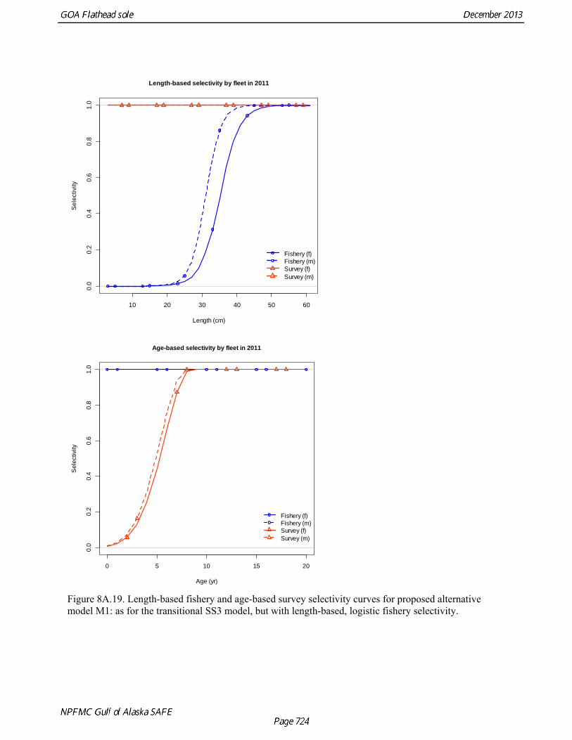
Figure 8A.19. Length-based fishery and age-based survey selectivity curves for proposed alternative model M1: as for the transitional SS3 model, but with length-based, logistic fishery selectivity.
10 20 30 40 50 60
0.0
0.2
0.4
0.6
0.8
1.0
Length-based selectivity by fleet in 2011
Length (cm)
Se
lect
ivity
Fishery (f)Fishery (m)Survey (f)Survey (m)
0 5 10 15 20
0.0
0.2
0.4
0.6
0.8
1.0
Age-based selectivity by fleet in 2011
Age (yr)
Sel
ect
ivity
Fishery (f)Fishery (m)Survey (f)Survey (m)

Figure 8A.20. Age-based double-normal fishery and survey selectivity for proposed alternative model M2 (as for the transitional SS3 model, but with an initial equilibrium fishing mortality rate estimated).
0 5 10 15 20
0.0
0.2
0.4
0.6
0.8
1.0
Age (yr)
Se
lect
ivity
Fishery (f)Fishery (m)Survey (f)Survey (m)
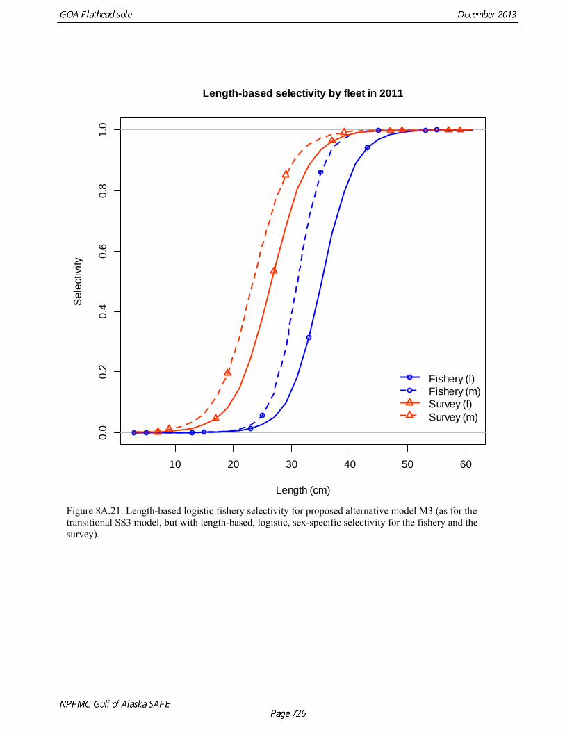
Figure 8A.21. Length-based logistic fishery selectivity for proposed alternative model M3 (as for the transitional SS3 model, but with length-based, logistic, sex-specific selectivity for the fishery and the survey).
10 20 30 40 50 60
0.0
0.2
0.4
0.6
0.8
1.0
Length-based selectivity by fleet in 2011
Length (cm)
Se
lect
ivity
Fishery (f)Fishery (m)Survey (f)Survey (m)

Figure 8A.22. Length-based fishery and survey selectivity for model M4 (as for the transitional SS3 model, but with estimation of an initial equilibrium fishing mortality rate and length-based, logistic, sex-specific selectivity for the fishery and the survey).
10 20 30 40 50 60
0.0
0.2
0.4
0.6
0.8
1.0
Length-based selectivity by fleet in 2011
Length (cm)
Se
lect
ivity
Fishery (f)Fishery (m)Survey (f)Survey (m)

Figure 8A.23. Comparison of numbers at age 3 for the 2011 model and proposed alternative model M4.
Year
Nu
mb
ers
at A
ge
3 (
in m
illio
ns)
01
00
20
03
00
40
0
1980 1985 1990 1995 2000 2005 2010
2011 Model
SS3

Figure 8A.24. Comparison of SSB (solid lines) and 95% asymptotic confidence intervals (dotted lines) for the 2011 assessment model and proposed alternative model M4.
Year
Sp
aw
nin
g s
tock
bio
ma
ss
02
00
00
40
00
06
00
00
80
00
01
00
00
0
1980 1985 1990 1995 2000 2005 2010
2011 ModelSS3
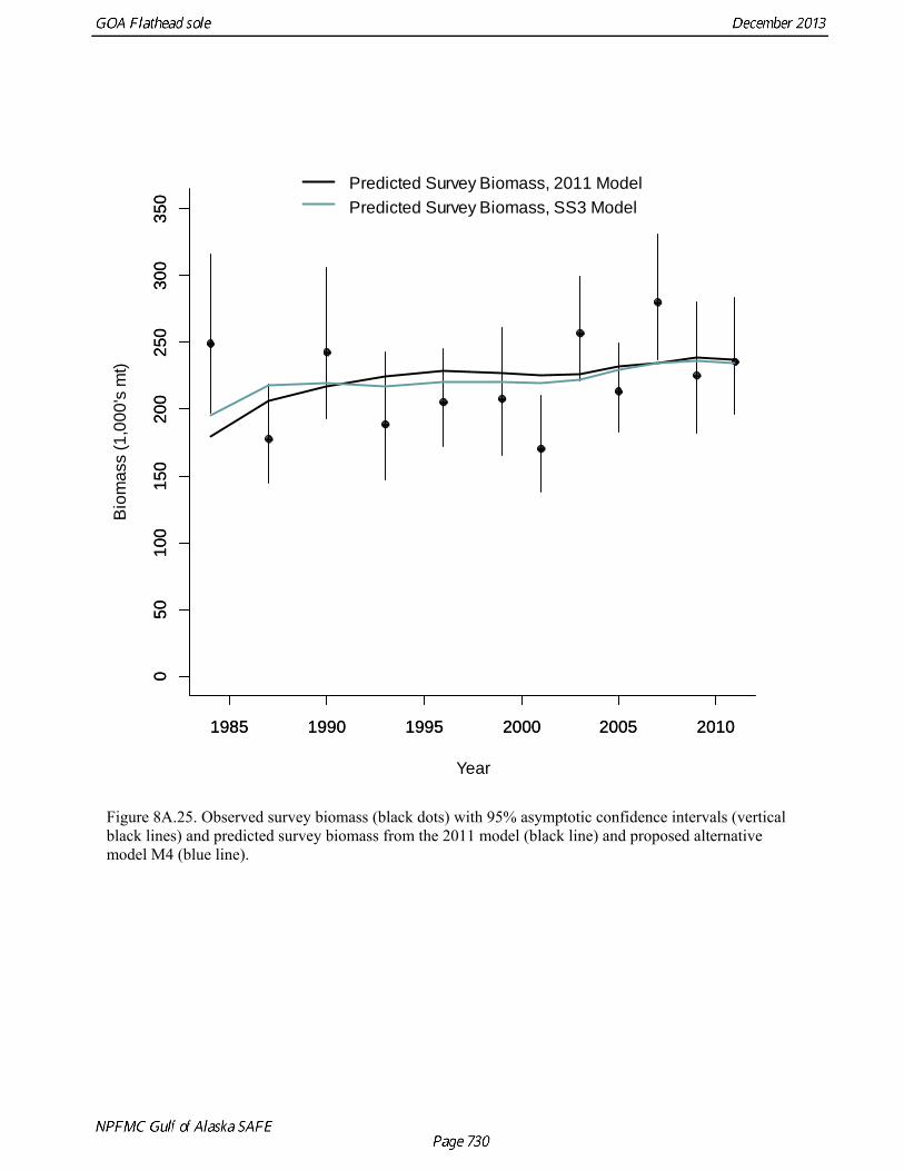
Figure 8A.25. Observed survey biomass (black dots) with 95% asymptotic confidence intervals (vertical black lines) and predicted survey biomass from the 2011 model (black line) and proposed alternative model M4 (blue line).
1985 1990 1995 2000 2005 2010
05
01
00
15
02
00
25
03
00
35
0
Year
Bio
ma
ss (
1,0
00
's m
t)
1985 1990 1995 2000 2005 2010
05
01
00
15
02
00
25
03
00
35
0Predicted Survey Biomass, 2011 Model
Predicted Survey Biomass, SS3 Model
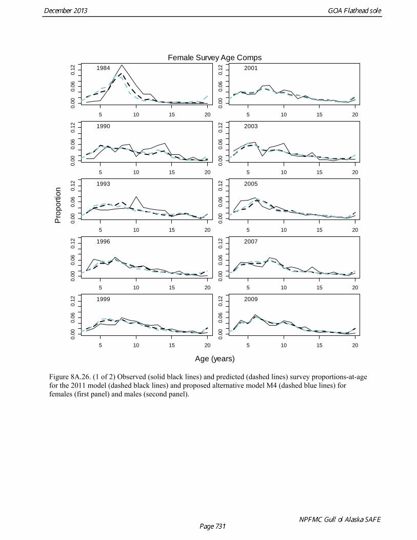
Figure 8A.26. (1 of 2) Observed (solid black lines) and predicted (dashed lines) survey proportions-at-age for the 2011 model (dashed black lines) and proposed alternative model M4 (dashed blue lines) for females (first panel) and males (second panel).
5 10 15 20
0.00
0.06
0.12 1984
5 10 15 20
0.00
0.06
0.12 1990
5 10 15 20
0.00
0.06
0.12 1993
5 10 15 20
0.00
0.06
0.12 1996
5 10 15 20
0.00
0.06
0.12 1999
5 10 15 20
0.00
0.06
0.12 2001
5 10 15 20
0.00
0.06
0.12 2003
5 10 15 20
0.00
0.06
0.12 2005
5 10 15 20
0.00
0.06
0.12 2007
5 10 15 20
0.00
0.06
0.12 2009
Age (years)
Pro
po
rtio
nFemale Survey Age Comps

Figure 8A.26. (2 of 2)
5 10 15 20
0.00
0.06
0.12 1984
5 10 15 20
0.00
0.06
0.12 1990
5 10 15 20
0.00
0.06
0.12 1993
5 10 15 20
0.00
0.06
0.12 1996
5 10 15 20
0.00
0.06
0.12 1999
5 10 15 20
0.00
0.06
0.12 2001
5 10 15 20
0.00
0.06
0.12 2003
5 10 15 20
0.00
0.06
0.12 2005
5 10 15 20
0.00
0.06
0.12 2007
5 10 15 20
0.00
0.06
0.12 2009
Age (years)
Pro
po
rtio
nMale Survey Age Comps

Figure 8A.27. (1 of 6) Observed (solid black lines) and predicted (dashed lines) fishery proportions-at-length for the 2011 model (dashed black lines) and proposed alternative model M4 (dashed blue lines) for females (first set of panels) and males (second set of panels).
20 30 40 50
0.00
0.15
1985
20 30 40 50
0.00
0.15
1986
20 30 40 50
0.00
0.15
1987
20 30 40 50
0.00
0.15
1988
20 30 40 50
0.00
0.15
1989
20 30 40 50
0.00
0.15
1990
20 30 40 50
0.00
0.15
1991
20 30 40 50
0.00
0.15
1992
20 30 40 50
0.00
0.15
1993
20 30 40 50
0.00
0.15
1994
20 30 40 50
0.00
0.15
1995
20 30 40 50
0.00
0.15
1996
Length (cm)
Pro
po
rtio
nFemale Fishery Size Comps

Figure 8A.27. (2 of 6)
20 30 40 50
0.00
0.15
1997
20 30 40 50
0.00
0.15
1998
20 30 40 50
0.00
0.15
1999
20 30 40 50
0.00
0.15
2000
20 30 40 50
0.00
0.15
2001
20 30 40 50
0.00
0.15
2002
20 30 40 50
0.00
0.15
2003
20 30 40 50
0.00
0.15
2004
20 30 40 50
0.00
0.15
2005
20 30 40 50
0.00
0.15
2006
20 30 40 50
0.00
0.15
2007
20 30 40 50
0.00
0.15
2008
Length (cm)
Pro
po
rtio
nFemale Fishery Size Comps

Figure 8A.27. (3 of 6)
20 30 40 50
0.00
0.15
2009
20 30 40 50
0.00
0.15
2010
20 30 40 50
0.00
0.15
2011
Length (cm)
Pro
po
rtio
nFemale Fishery Size Comps

Figure 8A.27. (4 of 6)
20 30 40 50
0.00
0.15
1985
20 30 40 50
0.00
0.15
1986
20 30 40 50
0.00
0.15
1987
20 30 40 50
0.00
0.15
1988
20 30 40 50
0.00
0.15
1989
20 30 40 50
0.00
0.15
1990
20 30 40 50
0.00
0.15
1991
20 30 40 50
0.00
0.15
1992
20 30 40 50
0.00
0.15
1993
20 30 40 50
0.00
0.15
1994
20 30 40 50
0.00
0.15
1995
20 30 40 50
0.00
0.15
1996
Length (cm)
Pro
po
rtio
nMale Fishery Size Comps

Figure 8A.27. (5 of 6)
20 30 40 50
0.00
0.15
1997
20 30 40 50
0.00
0.15
1998
20 30 40 50
0.00
0.15
1999
20 30 40 50
0.00
0.15
2000
20 30 40 50
0.00
0.15
2001
20 30 40 50
0.00
0.15
2002
20 30 40 50
0.00
0.15
2003
20 30 40 50
0.00
0.15
2004
20 30 40 50
0.00
0.15
2005
20 30 40 50
0.00
0.15
2006
20 30 40 50
0.00
0.15
2007
20 30 40 50
0.00
0.15
2008
Length (cm)
Pro
po
rtio
nMale Fishery Size Comps

Figure 8A.27. (6 of 6)
20 30 40 50
0.00
0.15
2009
20 30 40 50
0.00
0.15
2010
20 30 40 50
0.00
0.15
2011
Length (cm)
Pro
po
rtio
nMale Fishery Size Comps

Figure 8A.28. (1 of 2) Observed (solid black lines) and predicted (dashed lines) survey proportions-at-length for the 2011 model (dashed black lines) and proposed alternative model M4 (dashed blue lines) for females (first set of panels) and males (second set of panels).
20 30 40 50
0.00
0.06
1984
20 30 40 50
0.00
0.06
1987
20 30 40 50
0.00
0.06
1990
20 30 40 50
0.00
0.06
1993
20 30 40 50
0.00
0.06
1996
20 30 40 50
0.00
0.06
1999
20 30 40 50
0.00
0.06
2001
20 30 40 50
0.00
0.06
2003
20 30 40 50
0.00
0.06
2005
20 30 40 50
0.00
0.06
2007
20 30 40 50
0.00
0.06
2009
20 30 40 50
0.00
0.06
2011
Length (cm)
Pro
po
rtio
nFemale Survey Size Comps
Length (cm)
Pro
po
rtio
nFemale Survey Size Comps
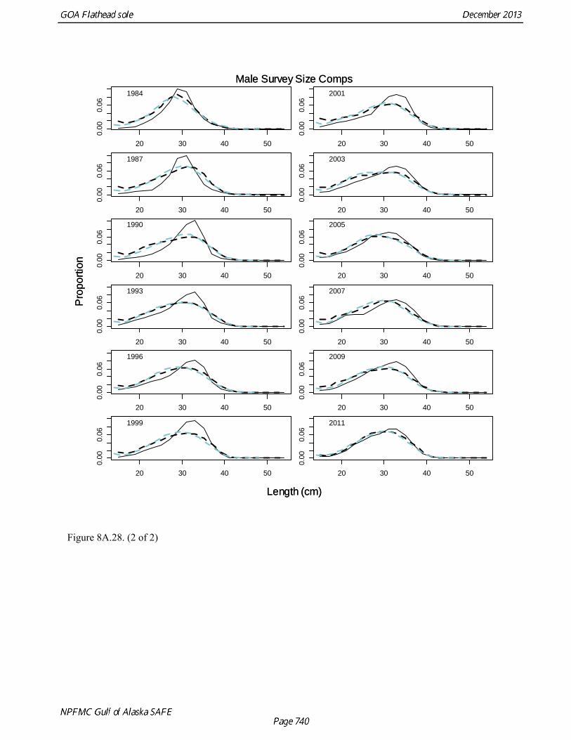
Figure 8A.28. (2 of 2)
20 30 40 50
0.00
0.06
1984
20 30 40 50
0.00
0.06
1987
20 30 40 50
0.00
0.06
1990
20 30 40 50
0.00
0.06
1993
20 30 40 50
0.00
0.06
1996
20 30 40 50
0.00
0.06
1999
20 30 40 50
0.00
0.06
2001
20 30 40 50
0.00
0.06
2003
20 30 40 50
0.00
0.06
2005
20 30 40 50
0.00
0.06
2007
20 30 40 50
0.00
0.06
2009
20 30 40 50
0.00
0.06
2011
Length (cm)
Pro
po
rtio
nMale Survey Size Comps
Length (cm)
Pro
po
rtio
nMale Survey Size Comps

Attachment 8b. A comparison of the previous assessment model updated with 2013 data to the current recommended assessment
model
The most recent accepted assessment model for GOA flathead sole (the 2011 model) was updated and run with 2013 data. This section compares the results of a run of the previous assessment model with 2013 data to the author’s recommended model for 2013. Below are executive summary tables that result from using the previous assessment model, projection model results based on the previous assessment model (Table 8B.1 – 8B.3), and plots comparing growth relationships, recruitment, spawning biomass, and fits biomass and composition data.
The key results of the 2013 assessment, based on the previous accepted assessment model, are compared to the key results of the accepted 2011 assessment model in the table below.
M (natural mortality rate) 0.2 0.2 0.2 0.2Tier 3a 3a 3a 3aProjected total (3+) biomass (t) 288,538 285,128 265,505 261,904Female spawning biomass (t) Projected Upper 95% confidence interval -- 96,799 95,773 Point estimate 106,377 107,178 96,782 95,714 Lower 95% confidence interval -- 96,768 95,661
B 100% 103,868 103,868 100,455 100,455
B 40% 41,547 41,547 40,182 40,182
B 35% 36,354 36,354 35,159 35,159
F OFL 0.593 0.593 0.56 0.56
maxF ABC 0.45 0.45 0.43 0.43
F ABC 0.45 0.45 0.43 0.43OFL (t) 61,036 62,296 54,641 54,511maxABC (t) 48,738 49,771 43,780 43,701ABC (t) 48,738 49,771 43,780 43,701
2011 2012 2012 2013Overfishing no n/a no n/aOverfished n/a no n/a noApproaching overfished n/a no n/a no
StatusAs determined in 2012 for: As determined in 2013 for:
Quantity
As estimated orspecified last year for:
As estimated orrecommended this year for:
2013 2014 2014 2015

Harvest Recommendations Based on the Previous Accepted Assessment
The reference fishing mortality rate for flathead sole is determined by the amount of reliable population information available (Amendment 56 of the Fishery Management Plan for the groundfish fishery of the Bering Sea/Aleutian Islands). Estimates of F40%, F35%, and SPR40% were obtained from a spawner-per recruit analysis. Assuming that the average recruitment from the 1983-2010 year classes estimated in this assessment represents a reliable estimate of equilibrium recruitment, then an estimate of B40% is calculated as the product of SPR40% times the equilibrium number of recruits. Since reliable estimates of the 2013 spawning biomass (B), B40%, F40%, and F35% exist and B>B40%, the flathead sole reference fishing mortality is defined in Tier 3a. For this tier, FABC is constrained to be ≤ F40%, and FOFL is defined to be F35%. The values of these quantities are:
The results of scenarios 6 & 7 indicate that the stock is not overfished and is not approaching an overfished condition. With regard to assessing the current stock level, the expected stock size in the year 2014 of scenario 6 is 96,782 t, more than 2 times B35% (35,159 t). Thus the stock is not currently overfished. With regard to whether the stock is approaching an overfished condition, the expected spawning stock size in the year 2026 of scenario 7 (36,882 t) is greater than B35%; thus, the stock is not approaching an overfished condition.
SSB 2013 96,782
B 40% 40,182
F 40% 0.43
maxFabc 0.43
B 35% 35,159
F 35% 0.56
F OFL 0.56

ATTACHMENT 8B TABLES
Table 8B.1. Projected spawning biomass based on the previous (2011) assessment model for the seven harvest scenarios listed in the “Harvest Recommendations” section
Table 8B.2. Projected fishing mortality rates based on the previous (2011) assessment model for the seven harvest scenarios listed in the “Harvest Recommendations” section
Year Scenario 1 Scenario 2 Scenario 3 Scenario 4 Scenario 5 Scenario 6 Scenario 72013 96,393 96,393 96,393 96,393 96,393 96,393 96,393 2014 96,782 96,782 96,782 96,782 96,782 96,782 96,782 2015 74,782 74,782 96,139 92,926 97,747 69,167 74,782 2016 59,929 59,929 94,687 88,769 97,741 52,520 59,929 2017 50,146 50,146 92,874 84,757 97,192 42,654 46,828 2018 44,154 44,154 91,139 81,312 96,522 37,244 39,540 2019 41,011 41,011 89,866 78,767 96,117 35,389 36,193 2020 39,796 39,796 89,118 77,119 96,053 35,412 35,665 2021 39,721 39,721 88,868 76,224 96,349 36,005 36,050 2022 40,001 40,001 88,904 75,787 96,827 36,530 36,511 2023 40,264 40,264 89,081 75,597 97,374 36,812 36,784 2024 40,420 40,420 89,265 75,499 97,861 36,906 36,886 2025 40,488 40,488 89,446 75,453 98,299 36,909 36,898 2026 40,509 40,509 89,574 75,410 98,632 36,887 36,882
Year Scenario 1 Scenario 2 Scenario 3 Scenario 4 Scenario 5 Scenario 6 Scenario 72013 0.02 0.02 0.02 0.02 0.02 0.02 0.022014 0.43 0.43 0.03 0.08 0.00 0.56 0.432015 0.43 0.43 0.03 0.08 0.00 0.56 0.432016 0.43 0.43 0.03 0.08 0.00 0.56 0.562017 0.43 0.43 0.03 0.08 0.00 0.56 0.562018 0.43 0.43 0.03 0.08 0.00 0.52 0.552019 0.43 0.43 0.03 0.08 0.00 0.49 0.502020 0.42 0.42 0.03 0.08 0.00 0.49 0.492021 0.42 0.42 0.03 0.08 0.00 0.50 0.502022 0.42 0.42 0.03 0.08 0.00 0.51 0.512023 0.42 0.42 0.03 0.08 0.00 0.51 0.512024 0.42 0.42 0.03 0.08 0.00 0.51 0.512025 0.42 0.42 0.03 0.08 0.00 0.51 0.512026 0.42 0.42 0.03 0.08 0.00 0.51 0.51

Table 8B.3. Projected catches based on the previous (2011) assessment model for the seven harvest scenarios listed in the “Harvest Recommendations” section
Year Scenario 1 Scenario 2 Scenario 3 Scenario 4 Scenario 5 Scenario 6 Scenario 72013 2,861 2,861 2,861 2,861 2,861 2,861 2,861 2014 43,780 43,780 3,038 9,121 - 54,641 43,780 2015 33,061 33,061 3,053 8,816 - 37,803 33,061 2016 25,821 25,821 3,036 8,461 - 27,693 32,310 2017 20,943 20,943 2,988 8,069 - 21,608 24,211 2018 17,803 17,803 2,923 7,681 - 16,926 19,254 2019 15,981 15,981 2,859 7,348 - 14,897 15,676 2020 14,953 14,953 2,811 7,109 - 14,728 14,976 2021 14,773 14,773 2,787 6,970 - 15,207 15,255 2022 14,926 14,926 2,782 6,904 - 15,695 15,679 2023 15,101 15,101 2,786 6,878 - 15,973 15,947 2024 15,212 15,212 2,793 6,869 - 16,073 16,054 2025 15,265 15,265 2,800 6,866 - 16,081 16,071 2026 15,278 15,278 2,806 6,864 - 16,061 16,056

ATTACHMENT 8B FIGURES
Figure 8B.1. Time series of spawning stock biomass (solid lines) and 95% asymptotic confidence intervals (dotted lines) for the recommended model (blue lines) and the previous assessment model (black lines).
Year
Spa
wni
ng s
tock
bio
mas
s0
4000
080
000
1200
00
1975 1985 1995 2005
2011 ModelSS3
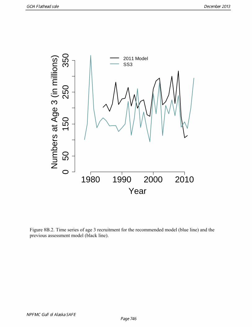
Figure 8B.2. Time series of age 3 recruitment for the recommended model (blue line) and the previous assessment model (black line).
Year
Num
bers
at A
ge 3
(in
mill
ions
)0
5015
025
035
0
1980 1990 2000 2010
2011 ModelSS3

Figure 8B.3. Fishery (top panel) and survey (bottom panel) selectivity at age by sex for the recommended model and previous model. Selectivity curves in the previous model are logistic and normalized so that maximum selectivity within the age range must equal 1.
0.0
0.2
0.4
0.6
0.8
1.0
0 5 10 15 20 25Age
Pro
port
ion
Fishery Selectivity
2011 Model, females2011 Model, malesSS3, femalesSS3, males
0.0
0.2
0.4
0.6
0.8
1.0
0 5 10 15 20 25Age
Pro
port
ion
Survey Selectivity
2011 Model, females2011 Model, malesSS3, femalesSS3, males

Figure 8B.4. (1 of 3) Observed (solid black lines) and predicted (dashed lines) fishery proportions-at-length for females for the current assessment model (blue dashed lines) and the previous assessment model updated with 2013 data (black dashed lines).

Figure 8B.4. (2 of 3)
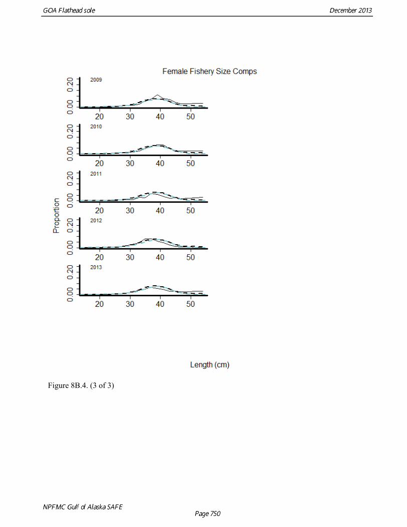
Figure 8B.4. (3 of 3)

Figure 8B.5. (1 of 3) Observed (solid black lines) and predicted (dashed lines) fishery proportions-at-length for males for the current assessment model (blue dashed lines) and the previous assessment model updated with 2013 data (black dashed lines).
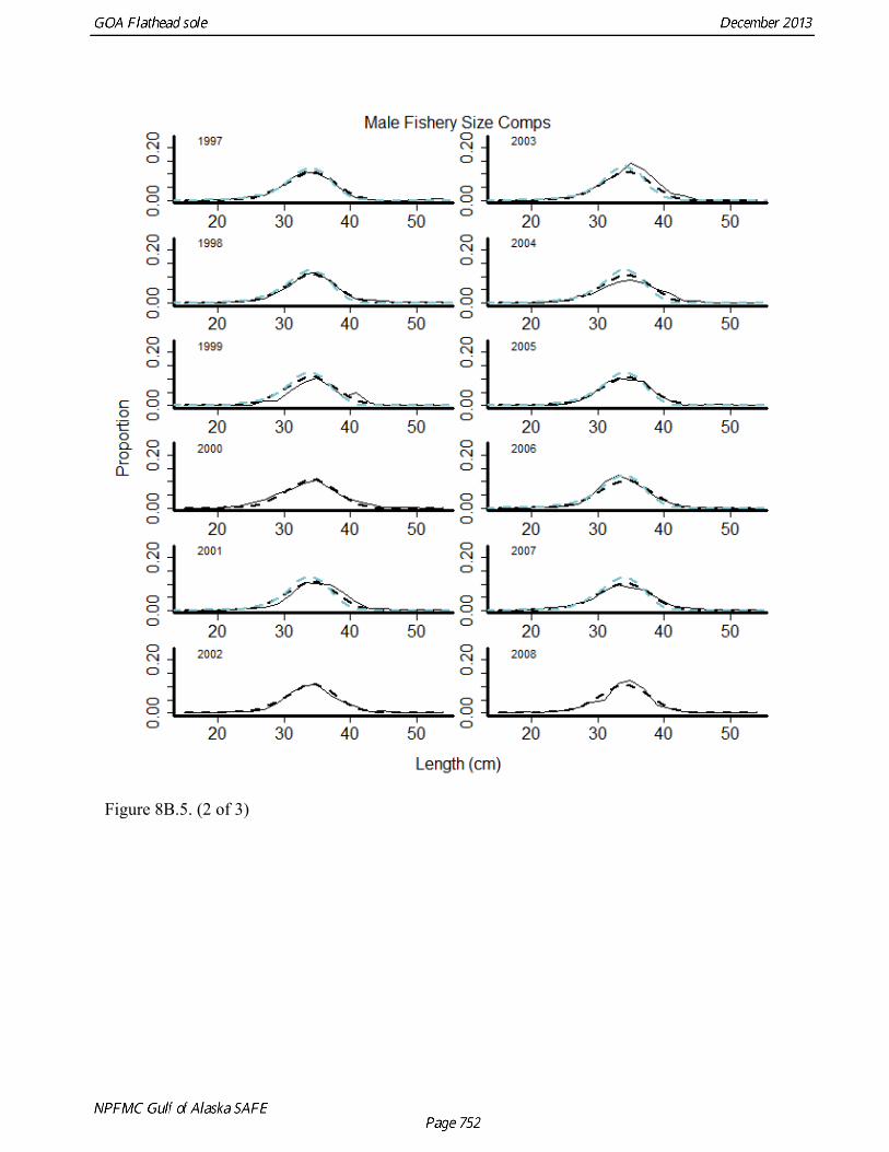
Figure 8B.5. (2 of 3)
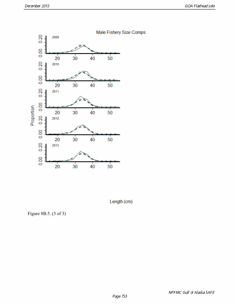
Figure 8B.5. (3 of 3)
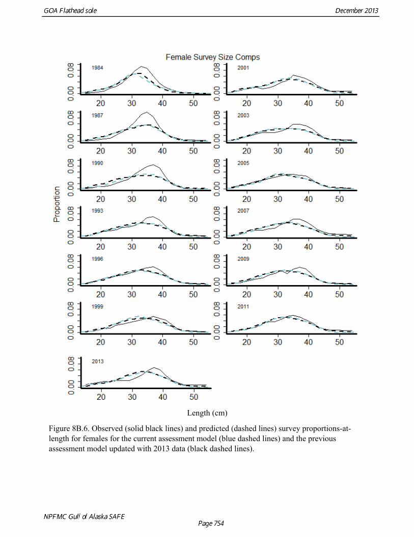
Length (cm)
Figure 8B.6. Observed (solid black lines) and predicted (dashed lines) survey proportions-at-length for females for the current assessment model (blue dashed lines) and the previous assessment model updated with 2013 data (black dashed lines).

Length (cm)
Figure 8B.7. Observed (solid black lines) and predicted (dashed lines) survey proportions-at-length for males for the current assessment model (blue dashed lines) and the previous assessment model updated with 2013 data (black dashed lines).

(This page intentionally left blank)