This electronic thesis or dissertation has been

downloaded from the King’s Research Portal at

https://kclpure.kcl.ac.uk/portal/

The copyright of this thesis rests with the author and no quotation from it or information derived from it

may be published without proper acknowledgement.

Take down policy

If you believe that this document breaches copyright please contact librarypure@kcl.ac.uk providing

details, and we will remove access to the work immediately and investigate your claim.

END USER LICENCE AGREEMENT

This work is licensed under a Creative Commons Attribution-NonCommercial-NoDerivatives 4.0

International licence. https://creativecommons.org/licenses/by-nc-nd/4.0/

You are free to:

Share: to copy, distribute and transmit the work Under the following conditions:

Attribution: You must attribute the work in the manner specified by the author (but not in any way that suggests that they endorse you or your use of the work).

Non Commercial: You may not use this work for commercial purposes.

No Derivative Works - You may not alter, transform, or build upon this work.

Any of these conditions can be waived if you receive permission from the author. Your fair dealings and

other rights are in no way affected by the above.

Low-energy Lorentz symmetry violation from quantum corrections in Lifshitz-scalingmodels

Brister, James Sebastian

Awarding institution:King's College London

Download date: 13. Jul. 2018

Low-energy Lorentz symmetry violation from

quantum corrections in Lifshitz-scaling models

James Brister

Department of Physics, King’s College London

A thesis submitted in fulfilment of the requirements

for the degree of Doctor of Philosophy in Physics

3rd of January, 2015

Abstract

In this thesis we investigate the effects of low-order quantum corrections on

Lifshitz-type quantum field theories. In particular, we consider the Lorentz-symmetry

violating corrections to the dispersion relations of the various particles of these the-

ories at low energies, which may be of a significant size even where the classical

effect is small.

We first study a Lifshitz scaling model of two fermion flavours in flat space,

interacting by a flavour mixing four-point term. We demonstrate the dynamical

generation of masses and flavour oscillations and consider these as a possible model

of neutrino mixing. We use existing experimental constraints on neutrino masses

and mixing angles to place restrictions on the couplings of our model. We then

investigate quantum corrections to the couplings and dispersions, and find that the

latter would be too large to be considered physical.

Next, we investigate a Lifshitz scaling model of Quantum Electrodynamics, con-

taining only fermions and gauge fields. We investigate the extent to which such

models may be phenomenologically viable, again primarily through calculating low-

order dressed dispersion relations. In doing this, we encounter issues not seen in

the simpler model such as those of gauge fixing and dimensional regularisation in

anisotropic theories. We again find that the dressed dispersion relations appear

notably non-relativistic even at low energies, despite the classical model being well

within experimental bounds.

Finally, we investigate the dressing of scalar and vector boson dispersion relations

by the quantum effects of the so-called “covariant” extension of Horava-Lifshitz

gravity, which despite having an unusual extra symmetry seems better behaved

than the “original” form of Horava gravity. We find that even integrating out

the effects of quantum gravity fluctuations alone gives significant corrections to the

matter sector’s dispersion relations, which allows us to place some new constraints

on the energy scales of the theory.

1

Declaration

I confirm that the work presented here is my own and that all references are

cited accordingly.

Chapter 5 contains work done in collaboration with Jean Alexandre and Nicholas

Houston and published in [1].

Chapters 6 and 8 contain work done in collaboration with Jean Alexandre and

published in [2] and [3].

2

Acknowledgements

I would like to thank my supervisor Jean Alexandre for his patience these past

years. I would also like to thank my fellow PhD students in the physics department

at King’s College, for putting up with my inane questions for so long; especially

Nicholas Houston, who bore the brunt of it.

3

Contents

1 Introduction 8

1.1 Motivations . . . . . . . . . . . . . . . . . . . . . . . . . . . . . . . . 8

1.2 Structure . . . . . . . . . . . . . . . . . . . . . . . . . . . . . . . . . 9

1.3 Notation and conventions . . . . . . . . . . . . . . . . . . . . . . . . 11

2 Background on Lorentz violation 13

2.1 Lorentz and Poincare symmetry . . . . . . . . . . . . . . . . . . . . . 13

2.2 Lorentz symmetry breaking . . . . . . . . . . . . . . . . . . . . . . . 14

2.3 Lorentz-violating models . . . . . . . . . . . . . . . . . . . . . . . . . 16

2.3.1 The Standard Model Extension . . . . . . . . . . . . . . . . . 16

2.3.2 “Top-down” models with Lorentz violation . . . . . . . . . . . 18

3 Effective actions and kinetic term dressing in Lorentz-violating the-

ories 19

3.1 Effective actions . . . . . . . . . . . . . . . . . . . . . . . . . . . . . . 19

3.1.1 Calculating effective actions . . . . . . . . . . . . . . . . . . . 19

3.1.2 Γ as a generating functional and diagrammatics . . . . . . . . 20

3.2 Calculating the dispersion relation corrections . . . . . . . . . . . . . 21

3.2.1 Effect on superficial divergences . . . . . . . . . . . . . . . . . 22

4 Lifshitz scaling in Quantum Field Theory 23

4.1 Introduction . . . . . . . . . . . . . . . . . . . . . . . . . . . . . . . . 23

4.2 Mass and spacetime dimensions . . . . . . . . . . . . . . . . . . . . . 24

4.3 Renormalisability . . . . . . . . . . . . . . . . . . . . . . . . . . . . . 25

4.4 Notable features of Lifshitz theories . . . . . . . . . . . . . . . . . . . 27

4.5 Other motivations for the study of Lifshitz theories . . . . . . . . . . 27

4.6 A worked example for effective actions in Lifshitz theories . . . . . . . 28

4.6.1 Model . . . . . . . . . . . . . . . . . . . . . . . . . . . . . . . 28

4.6.2 Calculation . . . . . . . . . . . . . . . . . . . . . . . . . . . . 28

4

5 Higher-order corrections

in a four-fermion Lifshitz model 31

5.1 Introduction . . . . . . . . . . . . . . . . . . . . . . . . . . . . . . . . 31

5.2 Flavour oscillations . . . . . . . . . . . . . . . . . . . . . . . . . . . . 32

5.2.1 Background: mechanisms for generating neutrino masses and

oscillations . . . . . . . . . . . . . . . . . . . . . . . . . . . . . 33

5.2.2 Flavour symmetry violating 4-fermion interactions . . . . . . . 35

5.2.3 Superficial degree of divergence . . . . . . . . . . . . . . . . . 36

5.2.4 Dynamical generation of masses . . . . . . . . . . . . . . . . . 36

5.2.5 Experimental constraints . . . . . . . . . . . . . . . . . . . . . 39

5.3 Asymptotic freedom . . . . . . . . . . . . . . . . . . . . . . . . . . . 40

5.3.1 One-loop Fermi coupling . . . . . . . . . . . . . . . . . . . . . 40

5.3.2 Beta-functions . . . . . . . . . . . . . . . . . . . . . . . . . . . 43

5.4 Two-loop propagator . . . . . . . . . . . . . . . . . . . . . . . . . . . 44

5.4.1 Self energy . . . . . . . . . . . . . . . . . . . . . . . . . . . . . 45

5.4.2 Dressed dispersion relations . . . . . . . . . . . . . . . . . . . 46

5.5 Conclusion . . . . . . . . . . . . . . . . . . . . . . . . . . . . . . . . . 47

6 Fermion effective dispersion relation for z = 2 Lifshitz QED 49

6.1 Introduction . . . . . . . . . . . . . . . . . . . . . . . . . . . . . . . . 49

6.2 Model . . . . . . . . . . . . . . . . . . . . . . . . . . . . . . . . . . . 50

6.2.1 Propagators and interactions . . . . . . . . . . . . . . . . . . . 51

6.2.2 Symmetries of the dressed propagators . . . . . . . . . . . . . 52

6.3 One-loop propagators . . . . . . . . . . . . . . . . . . . . . . . . . . . 54

6.3.1 IR behaviour . . . . . . . . . . . . . . . . . . . . . . . . . . . 54

6.3.2 UV behaviour . . . . . . . . . . . . . . . . . . . . . . . . . . . 54

6.3.3 One-loop corrections . . . . . . . . . . . . . . . . . . . . . . . 55

6.3.4 Phenomenology . . . . . . . . . . . . . . . . . . . . . . . . . . 56

6.4 Conclusion . . . . . . . . . . . . . . . . . . . . . . . . . . . . . . . . . 57

7 Horava-Lifshitz gravity 58

7.1 Introduction . . . . . . . . . . . . . . . . . . . . . . . . . . . . . . . . 58

7.2 Model . . . . . . . . . . . . . . . . . . . . . . . . . . . . . . . . . . . 59

7.3 Restrictions . . . . . . . . . . . . . . . . . . . . . . . . . . . . . . . . 60

7.3.1 Detailed Balance . . . . . . . . . . . . . . . . . . . . . . . . . 60

7.3.2 Projectability . . . . . . . . . . . . . . . . . . . . . . . . . . . 61

7.4 Problems . . . . . . . . . . . . . . . . . . . . . . . . . . . . . . . . . . 61

7.4.1 Scalar graviton . . . . . . . . . . . . . . . . . . . . . . . . . . 61

7.4.2 Quantisation and interactions . . . . . . . . . . . . . . . . . . 63

5

7.5 Expansion about flat space . . . . . . . . . . . . . . . . . . . . . . . . 64

7.5.1 Constraints . . . . . . . . . . . . . . . . . . . . . . . . . . . . 64

7.5.2 Gauge fixing . . . . . . . . . . . . . . . . . . . . . . . . . . . . 64

7.5.3 Equations of motion . . . . . . . . . . . . . . . . . . . . . . . 65

7.6 Cosmological bounds . . . . . . . . . . . . . . . . . . . . . . . . . . . 65

7.7 Covariant Horava-Lifshitz gravity . . . . . . . . . . . . . . . . . . . . 66

7.7.1 Symmetries and Lagrangian . . . . . . . . . . . . . . . . . . . 66

7.7.2 Degree of freedom counting . . . . . . . . . . . . . . . . . . . 66

7.7.3 Problems . . . . . . . . . . . . . . . . . . . . . . . . . . . . . 67

7.7.4 Other work . . . . . . . . . . . . . . . . . . . . . . . . . . . . 67

7.8 Relating HL gravity to other modified gravity models . . . . . . . . . 67

7.8.1 Einstein-Aether and khronometric models . . . . . . . . . . . 67

7.8.2 Dark matter free models . . . . . . . . . . . . . . . . . . . . . 68

8 Effective matter dispersion relation in quantum

covariant Horava-Lifshitz gravity 71

8.1 Introduction . . . . . . . . . . . . . . . . . . . . . . . . . . . . . . . . 71

8.2 Review of covariant Horava-Lifshitz gravity . . . . . . . . . . . . . . . 72

8.2.1 Notation . . . . . . . . . . . . . . . . . . . . . . . . . . . . . . 72

8.2.2 The action . . . . . . . . . . . . . . . . . . . . . . . . . . . . . 72

8.2.3 Gauge fixing and U(1)-symmetry constraints . . . . . . . . . . 74

8.3 Effective dispersion relation for matter fields . . . . . . . . . . . . . . 74

8.3.1 Coupling to matter . . . . . . . . . . . . . . . . . . . . . . . . 74

8.3.2 Features of the one-loop integration . . . . . . . . . . . . . . . 75

8.3.3 Integration . . . . . . . . . . . . . . . . . . . . . . . . . . . . 77

8.4 Analysis and conclusions . . . . . . . . . . . . . . . . . . . . . . . . . 79

8.4.1 Analysis . . . . . . . . . . . . . . . . . . . . . . . . . . . . . . 79

8.4.2 Conclusions . . . . . . . . . . . . . . . . . . . . . . . . . . . . 79

9 Conclusions 82

9.1 Summary . . . . . . . . . . . . . . . . . . . . . . . . . . . . . . . . . 82

9.2 Analysis . . . . . . . . . . . . . . . . . . . . . . . . . . . . . . . . . . 83

9.2.1 Dressed dispersion relations . . . . . . . . . . . . . . . . . . . 83

9.2.2 Mass scales . . . . . . . . . . . . . . . . . . . . . . . . . . . . 84

9.3 Further Work . . . . . . . . . . . . . . . . . . . . . . . . . . . . . . . 85

A Two-loop propagator in the 4-fermi model 87

B Details of loop integrals in z = 2 QED 91

B.1 Photon mass . . . . . . . . . . . . . . . . . . . . . . . . . . . . . . . . 91

6

B.2 Fermion corrections . . . . . . . . . . . . . . . . . . . . . . . . . . . . 92

B.3 Photon corrections . . . . . . . . . . . . . . . . . . . . . . . . . . . . 93

C Dimensional Regularisation 94

C.1 Finiteness of naıvely divergent integrals . . . . . . . . . . . . . . . . . 94

C.2 Divergence cancelling . . . . . . . . . . . . . . . . . . . . . . . . . . . 95

7

Chapter 1

Introduction

1.1 Motivations

A severe restriction often imposed on a quantum field theory (QFT) is the re-

quirement, if the theory is to be treated as anything other than an effective approx-

imation, that it be renormalisable into the far ultraviolet; in practice, we usually

require our models to be perturbatively renormalisable, as this is generally our only

practical way of calculating meaningful results.

The majority of observed phenomena can be accounted for by the Standard

Model of particle physics, which is believed to be renormalisable, plus the theory

of General Relativity (GR). However, GR, treated as a perturbative quantum field

theory about some background metric, fails to be perturbatively renormalisable and

so (for this reason, and complications arising from curved spacetime) cannot be

readily treated as a QFT. Barring the possibility of some non-gaussian fixed point,

to which the theory may flow in the ultra-violet without it being detectable per-

turbatively (the “Asymptotic Safety” scenario), one therefore expects the present

models of gravity to break-down in some way above a certain energy scale, perhaps

requiring something “beyond” standard relativistic QFT.

Lorentz symmetry, global or local, is a well-founded and well-tested character-

istic of all our current predictive models of fundamental physics, over a wide range

of scales. However, it is a relatively simple thing to break, either deliberately or

through some unexpected condensation; indeed, many speculative models of more

fundamental physics involve some degree of Lorentz symmetry violation, usually

appearing at very high energies so as not to produce effects at experimental energies

that should already have been observed.

A type of Lorentz violating model of that has garnered interest lately, and is the

8

primary focus of this study, is those with so-called Lifshitz scaling. In these models

there is a preferred choice of time co-ordinate, which has differing mass dimension

and asymptotic scaling to the spatial co-ordinates. These models are of interest as

they allow many more interactions in quantum field theories to become renormal-

isable. In particular, a recent proposal by Horava [4] for a Lifshitz-scaling model

of gravity, appears to be perturbatively renormalisable, at least by power-counting;

such a model, if it could be made to approximate GR at experimental energies (a

non-trivial condition), would allow us to treat gravity with our usual methods of

perturbative QFT.

Throughout this thesis, we shall see that it is not as easy to sequester Lorentz-

violating effects away at high energies as is often assumed. We shall investigate

various models with Lifshitz scaling (and several of the usually non-renormalisable

interactions that would not be allowed in a Lorentz invariant model) and calculate

low-order quantum corrections to some important processes, we shall focus especially

on the anisotropic corrections to the propagation relations of the various species

of particle in the models as these may lead to readily observable deviations from

relativistic behaviour. We shall find repeatedly that quantum considerations give

much stronger constraints on the scales of Lorentz violation than a purely classical

analysis would suggest.

1.2 Structure

We begin by introducing the theoretical concepts behind Lorentz violating mod-

els and some of the techniques used to study these. We discuss Lifshitz-scaling

models in flat spacetime. We then study a model of fermions, taken to represent

neutrinos, with an interaction that would not be allowed in an isotropic theory.

We demonstrate the dynamical generation of masses and flavour oscillations in this

model and calculate lowest-order quantum corrections to the propagation relations.

We find that the induced low-energy Lorentz violation will likely be too large to be

realistic, without significant fine-tuning.

We then study similar effects in a more complex model: a Lifshitz-scaling version

of quantum electrodynamics, with one fermion coupled to a U(1) gauge field. We see

that the simultaneous imposition of Lifshitz scaling and gauge symmetry introduces

new interactions and complicates gauge fixing. We examine some unusual features

of the method of dimensional regularisation (that we adopt here as it preserves the

gauge symmetry) that one would not see in isotropic QED.

At this point we discuss Lifshitz scaling in curved spacetime and introduce

Horava-Lifshitz gravity (and its various extensions and modifications). We then

9

perform a similar analysis to the first two studies in the “covariant” extension of

Horava-Lifshitz gravity, in which an extra U(1) symmetry is introduced to restore

the number of propagating degrees-of-freedom per spacetime point to its relativistic

value. We study this model coupled to “normal” classical Lorentz-invariant matter

and integrate out quantum metric fluctuations about flat space to produce an ef-

fective action for the matter. We again find a significant Lorentz-violating effect at

low energies which can be used to further restrict the range of possible parameters

of such models; in particular the scale of Lorentz violation is given bounds that are

physically reasonable.

The structure of this thesis is as follows:

• In chapter 2 we introduce the basic concepts behind Lorentz violation in gen-

eral, and discuss various models that exhibit such behaviour.

• In chapter 3 we discuss the effective action methods that we shall use repeat-

edly in subsequent chapters

• In chapter 4 we consider Lifshitz models in particular and examine their un-

usual features, including the mechanisms by which they improve the renor-

malisability of QFTs.

• In chapter 5 we examine a Lifshitz model for two species of fermion, with a

flavour-mixing 4-point interaction that would be nonrenormalisable in a rel-

ativistic theory. We calculate one-loop corrections to the propagation speed

and examine the dynamical generation of masses and flavour oscillations.

• In chapter 6 we perform a similar analysis for a more realistic abelian gauge

theory, containing both fermions and gauge bosons. We find corrections to

apparent low-energy propagation speeds, with some interesting mathemati-

cal features, which may impose restrictions on the allowed parameters of the

model.

• In chapter 7 we discuss the violation of local Poincare symmetry in the con-

text of Horava’s Lifshitz-scaling model of gravity; its assumptions, experimen-

tal bounds, the several versions that have been more recently proposed and

their various issues. We also relate Horava’s model to other modified gravity

scenarios.

• In chapter 8, we consider so-called “covariant” Horava-Lifshitz gravity coupled

to relativistic matter and integrate out the effects of gravitational fluctuations

about flat space; again we obtain modified propagation relations that allow

10

us to restrict several parameters of the model by comparison to experimental

data.

• Chapter 9 contains a summary of the work, concluding remarks and potential

directions for further studies.

• This thesis includes three appendices; the first two detail longer calculations

omitted from chapters 5 and 6. The final appendix discusses some unusual

features of the method of dimensional regularisation.

1.3 Notation and conventions

If not specified otherwise, we shall assume that we are working in 3+1 spacetime

dimensions.

As we shall be discussing the violation of Lorentz symmetry, we shall need to

distinguish space and time co-ordinates: we use lower-case Greek indices, µ, ν . . .,

for the components of spacetime tensors, lower-case Latin indices, i, j, . . . for spatial

tensors (or spatial components of spacetime tensors) and 0 for time components.

We adopt the usual summation conventions over repeated indices, for both space

and spacetime tensors.

We take ∆ = ∂i∂i to be the spatial Laplacian. Similarly for a 4-vector kµ =

(k0, ki) we write k as the magnitude of its spatial part. We will generally adopt the

convention that c = 1 = ~ and use the mostly-minus metric signature (such that

kµkµ = k2

0 − k2). We shall occasionally write a spatial vector as ~k, where we feel it

may be confused with a scalar.

Curved spacetime

In discussions of Horava-Lifshitz gravity, we shall adopt the mostly-plus conven-

tion more commonly used by others in the field of quantum gravity (and general

relativity in general), in order to avoid confusion when comparing our work to that

of other authors. We shall, of course, make very clear when this change of conven-

tion is happening.

In curved spacetime, we shall need to distinguish spatial tensors contracted with

the ADM 3-metric gij from those contracted with the flat-space 3-metric δij. For

two vectors vi, wi, we will write the former as viwi and the latter as viwi, which

11

leads to vµwµ = −v0w0 + viwi, where

viwi = viwjgij ,

gijgjk = δik . (1.1)

Also, we denote v2 = vivi, we use ∂i for the flat 3-space derivative, and ∂2 for the

flat 3-space Laplacian.

12

Chapter 2

Background on Lorentz violation

In this chapter we introduce the basic features of Lorentz symmetry and the

various effects of its violation, such as the non-relativistic propagation that will

be the main focus of this thesis. Finally, we examine several models that include

Lorentz violation, including the “Standard Model Extension” that can be taken as

a parametrisation of most Lorentz-violating terms.

2.1 Lorentz and Poincare symmetry

The Lorentz group is the maximal set of linear transformations that preserve

the Minkowski metric ηµν = diag1,−1,−1,−1 and the origin; its generators are

antisymmetric matrices Mµν obeying

[Mµν ,Mρσ] = i(Mµρηνσ +Mνσηµρ −Mµσηνρ −Mνρηµσ) . (2.1)

Equivalently, the (proper, orthochronous) Lorentz group is the unique set of sym-

metries such that a linear transformation relates different inertial frames in a re-

versible and isotropic fashion, depending only on the velocity, while preserving a

constant speed (that of massless particles). The Galilean transformations of New-

tonian physics can be considered the c→∞ limit of the Lorentz transformations.

With the addition of the generators of space-time translations, Pµ, these form the

Poincare algebra:

[Pµ, Pν ] = 0, [Mµν , Pρ] = i(ηµρPν − ηνρPµ). (2.2)

We shall follow most of the literature in referring primarily to “Lorentz symme-

try” and “Lorentz violation”, rather than Poincare symmetry; the non-invariance

of physical laws under translation is not often considered. This distinction becomes

slightly more important when considering local Poincare symmetry and its possible

violations.

13

2.2 Lorentz symmetry breaking

Conceptually, the violation of Lorentz symmetry is very easy. One can simply

add some coupling to a constant non-Lorentz-invariant background field, such as a

constant vector or spinor, to an existing model (or one can introduce a potential

that will generate the same spontaneously). Generally, when “Lorentz violation” is

mentioned, what is meant is a violation of invariance under the boost transformations

(i.e. the generators M0i) in some frame; this could be justified by noting that

the natural parameter for boosts is the relative velocity which, unlike the angle of

rotation associated with the Mij, cannot be so readily tested throughout its whole

range or, relatedly, that large boosts for massive objects necessarily contain a high

energy scale, which could lead to effects unobserved at typical experimental energies.

Generally, while breaking boosts produces an asymmetry between space and

time, it does not restore the Galilean symmetry of Newtonian dynamics. Without

additional assumptions, the Poincare group will simply be broken into the SO(3)

of spatial rotations, plus space and time translations. This sort of Lorentz breaking

suggests there is a preferred rest frame in which “space” and “time” co-ordinates

may be separated 1; in most such models, this may be taken to be the rest frame

of the Cosmic Microwave Background (CMB), unless some frame-dragging effect is

invoked. However, most experimental searches for Lorentz violation adopt a more

convenient Sun-centred frame.

There are several other generic properties of theories without boost symmetry.

One is that if the Lorentz breaking terms are coupled to one species of particle but

not another (or with different strengths), then propagation relations may differ be-

tween those species (in ways other than the usual differing masses), such as differing

effective “speeds of light” which will be discussed in more detail below. Alternatively,

the propagation relation of even a single species may become energy-dependent in

a way other than the expected

ω2 = m2 + k2 , (2.3)

where the frequency ω = k0. In fact, energy-dependent propagation relations may

allow one to construct models in which propagation is approximately relativistic at

low energies (where we have measured it) while being highly Lorentz-violating at

higher scales. Such a model would come at the cost of introducing at least one

1For instance, if there were a time- or space-like background vector, the frame in which it has

no space or time components (respectively) would seem to be a natural rest frame. It should be

noted that such a vector is not sufficient to define a global foliation of a spacetime into space-like

surfaces. A null background vector may well violate Lorentz invariance, but not give a preferred

rest frame.

14

typical energy scale to the model. For example, a particle with the propagation

relation

ω2 = m2 + k2 +k4

M2(2.4)

would appear Lorentz invariant when k M , but not when k M . Such relations

are common in the Lifshitz models we shall discuss later.

A distinction should be made between Lorentz violation in classical and quantum

field theories. In the former, it is relatively simple to confine Lorentz-violating effects

to a few (weakly-interacting) species or very high energies but once quantum effects

are taken into account this becomes significantly more difficult: loop corrections

involve integrating over arbitrarily high loop momenta, so “high energy” effects

from non-Lorentz-invariant propagators may appear even at low energies (suppressed

by powers of ~, but that may not be sufficient to render them unobservable at

experimental energies).

Of particular relevance to the present study are quantum corrections to low-

energy dispersion relations. Without Lorentz invariance, the time- and space-

derivative terms in the kinetic part of the action for some particle may be dressed

differently, leading to a dispersion relation of the form

Aω2 = m2 +Bk2 . (2.5)

In relativistic QFT, one would have A = B, and so this correction could be absorbed

by a re-definition of the field strengths (this is the usual “wavefunction renormal-

isation” of QFT); clearly, that is not possible here. Of course, one could always

perform a re-scaling of space or time to restore the usual relativistic dispersion re-

lation (while modifying the mass). However, if one had two or more species that

are dressed differently, performing such a rescaling for both species simultaneously

would be impossible. Such a scenario leads to the two species having dispersion

relations

ω21 = m2

1 + k21,

ω22 = m2

2 + Ak22. (2.6)

The two species have different effective “speeds of light” (1 and√A respectively)2

and associated “light cones” [5]. As these are quantum corrections, they may run

with energy, leading additionally to an energy dependence in the propagation.

It should be noted that without the full Poincare symmetry, the energy-momentum

tensor is not a conserved quantity, though any of its components may be, separately,

2Though the choice of which species’ speed to set to 1 is, of course, arbitrary.

15

depending on the remaining symmetries.

It should also be noted that any violation of CPT invariance would also imply

Lorentz violation [6].

2.3 Lorentz-violating models

2.3.1 The Standard Model Extension

In [7], the authors have collected experimental restrictions on the coefficients

of the so-called Standard Model Extension (SME), an effective theory consisting

of the Standard Model of particle physics, general relativity and all possible rele-

vant Lorentz- or Poincare-violating operators, for both the Standard Model fields

and gravity [8]; the coefficients of these operators therefore provide an effective

parametrisation of possible Lorentz-violating effects.

For instance, if we restrict our attention to a single fermion, ψ, in flat spacetime, a

minimal model that includes dimension 3 and 4 operators would give a Lagrangian

density of

LLV = ψ(Aµνσ

µν

+ aµγµ + bµγ5γ

µ

+ cµνγµDν + dµνγ5γ

µDν

+ eµDµ + fµγ5D

µ + gµνξσµνDξ

)ψ , (2.7)

in addition to the usual kinetic and mass terms. The coefficients A, a, b, c, d, e, f, g

are arbitrary tensors that may not be Lorentz invariant (indeed several of them, by

symmetry, cannot be unless they are zero) and Dµ is the covariant derivative under

whatever gauge symmetries the model may possess. Note that only the terms on

the second and fourth rows above violate CPT invariance.

Even the simple model above contains 78 scalar parameters, so it should be clear

that the more general SME can contain a very large number of terms, especially once

higher-dimension operators are allowed. The most readily measured dimensionless

coefficients can be seen to be of order 10−15 at most, so any Lorentz violating effect

must either be negligible at current experimental energies or affect only hard-to-

measure processes.

The data from which these limits are derived come from a wide variety of sources

including

16

• astrophysical data such as time-of flight measurements from supernovae and

quasars

• precision measurements of cold atoms and optical resonators

• vacuum birefringence measurements from distant light sources

• Earth-based experiments searching for annual variations in physical processes

• direct tests for CPT violation and other collider physics.

The references in [7] provide a fairly comprehensive list of experiments that we shall

not repeat here. Instead we shall examine one particular example in some detail

below, to illustrate the typical concepts.

Example test of SME parameters - electrodynamics

In [9], the authors examine a Lorentz-violating extension to the gauge sector

of electrodynamics, with the aim of designing an experiment to improve the ex-

isting bounds on such models, their model is parametrised by the 23 independent

parameters of a and b in

LLV = aµνρσFµνF ρσ + bλελµνρA

µF νρ , (2.8)

and they find that all but three of these parameters can be restricted to be less than

10−37 simply by the non-observation of birefringence effects from distant astrophys-

ical sources; in fact the components of b must be less than 10−42 GeV. The three

remaining three parameters are the components of

vi =1

2(a0kik − a0kki) (2.9)

which are “only” constrained to be less than 10−11, from optical cavity experi-

ments. Setting the other, more restricted terms to zero, the authors then calculate

the alterations to Maxwell’s equations: they find that a non-zero vi will produce

a magnetic field from a static charge, and an electric field from a steady current.

Having determined this, the authors conclude that such an effect would be easily

observed in charged particle beam interference experiments; they describe a simple

beam splitting and re-combination experiment in which the presence of vi induces

a path-dependent phase shift that is, in principle, measurable and should allow one

to improve the bound on the vi by one or two orders of magnitude, given reasonable

experimental accuracies.

It should be noted that this experiment measures Lorentz violation in the QED

sector, where particles are comparatively strongly interacting and easily observed.

17

Constraints for more weakly coupled fields, such a neutrinos and the gravity sector,

tend to be looser. In chapter 7, we shall examine results from such an effective

model, derived from Horava-Lifshitz gravity.

2.3.2 “Top-down” models with Lorentz violation

The SME discussed above is only an effective phenomenological model. We will

now briefly describe two more “fundamental” Lorentz-violating models, motivated

by theoretical concerns, that may be related to the Lifshitz theories that are the

main focus of this study.

Any model that attempts to discretise space and time will violate Lorentz in-

variance: there is no possible Lorentz invariant regular lattice, nor (under certain

reasonable assumptions) can there be a Lorentz invariant random distribution of

points [10]. In particular, the approach of Causal Dynamical Triangulations is to

approximate continuous spacetime with a discrete network of simplices, such that

all the “curvature” is contained in the deficit angles between triangles [11][12]. In

[12] a phase of spacetime in Causal Dynamical Triangulations is found that appears

to be singular unless one imposes Lifshitz-like scaling in the limit approaching it.

Doubly Special Relativity [13] refers to a collection of models that preserve a sec-

ond fundamental scale, normally taken to be the Planck energy. Generically, these

theories lead to energy-dependent dispersion relations. Doubly General Relativity

or Rainbow Gravity [14] is an extension of these ideas to curved spacetime (in [15]

a correspondence between Doubly General Relativity and Horava gravity is estab-

lished).

Other models, such as Einstein-Aether gravity, are best examined as theories in

curved spacetime, and so we shall delay their discussion until we have introduced

Horava-Lifshitz gravity in chapter 7.

18

Chapter 3

Effective actions and kinetic term

dressing in Lorentz-violating

theories

In this chapter, we introduce effective actions and describe a few of the mathe-

matical notions and techniques that will be of use in later chapters.

3.1 Effective actions

When we discuss an “effective action” here we shall usually mean it in the sense

of an action for a classical field that gives the expectation of the equivalent quantum

field. Given a generating functional, Z[J ] for a QFT, which we shall take to have

just one scalar field, φ(x, t) for simplicity (and thus only one source term J(x, t))

Z[J ] =

∫Dφei(S(φ)+

∫d3xdtJφ) . (3.1)

We define W [J ] = i logZ[J ] which is, by simple analysis of the properties of the ex-

ponential, the generating functional of connected correlation functions. The effective

action we define by

Γ[φc] = −W [J ]−∫d3xdtJφc (3.2)

where φc(x, t) = − δW [J ]δJ(x,t)

is the expectation of φ and can be considered the classical

field.

3.1.1 Calculating effective actions

Of course, calculating Γ exactly would be equivalent to solving the theory 1,

which is not tractable in most cases. We instead approximate the action to one or

1as one would “simply” have an extremely non-linear classical field theory in which to calculate

19

two loop order.

Let the action S, be an integral of some classical Lagrangian density (that is,

without renormalisation counterterms), L. We attempt to calculate the effective

action perturbatively; we write φ = φc + ϕ, where ϕ represents fluctuations about

the classical solution. We can now represent Z[J ] by∫Dϕ exp(i

∫d3xdt[L(φc) + Jφc + (0)ϕ+

∫d3x′dt′

1

2ϕϕ′

δ2Lδφδφ′

+ . . .]) (3.3)

where φ′, ϕ′ are functions of x′, t′, the terms linear in ϕ vanish by the definition of

φc and all functional derivatives are evaluated at φc(x). The ellipsis represents both

higher order terms in ϕ and possible renormalisation counterterms.

If we truncate this expansion at order ϕ2, we may perform the path integral

exactly (as it is a Gaussian integral). We obtain

Z[J ] ' exp(i

∫d3xdt[L(φc) + Jφc).(det[− δ2L

δφ(x)δφ(x′)])−1/2, (3.4)

where a functional determinant can be suitably defined as

det f(x, y) = exp Tr log f(x, y)

Tr[f(x, y)] =

∫ddxddyf(x, y)δ(x− y) (3.5)

Once we have evaluated this determinant, and added any necessary counterterms 2,

δL, our first order approximation to the effective action can be written as

Γ1[φc] =

∫d3xdt[L+ δL](φc) +

i

2log det[− δ2L

δφ(x)δφ(x′)φ=φc

]. (3.6)

Iterating this process would produce higher-order corrections. In practice, calcu-

lating even this approximation to the full effective action is often not necessary, as

the information one seeks can be found by making simplifying assumptions (such as

constant φc to find the effective potential for the ground state).

3.1.2 Γ as a generating functional and diagrammatics

Given thatδ2W [J ]

δJ(x)δJ(x′)= −iD(x, x′) (3.7)

2in particular, to remove tadpole terms, which would invalidate our assumption that ϕ is per-

turbative

20

gives the propagator, by the chain rule and the definition of φc we have

δ

δJ(x)=

∫dy iD(x, y)

δ

δφc(y)(3.8)

and alsoδ2Γ[φc]

δφc(x)δφc(x′)= iD−1(x, x′) . (3.9)

Considering a third derivative of W (i.e a connected 3-point function), one obtains

δ3W [J ]

δJ(x)δJ(y)δJ(z)=

∫dudvdw iD(x, u)D(v, y)D(w, z)

δ3Γ[φc]

δφc(u)δφc(v)δφc(w)(3.10)

that is to say, the third functional derivative of Γ gives the connected three-point

function with the external propagators removed i.e the one-particle irreducible three

point function. One can iterate this calculation for higher derivatives of W , where

one can see by simple induction that Γ[φc] is indeed the generating functional of one-

particle-irreducible correlation functions. This is extremely useful, as it allows one

to rapidly determine the relevant terms for an n-loop approximation to the effective

action, simply from 1PI Feynman diagrams.

3.2 Calculating the dispersion relation corrections

We can now expand

Γ[φc] =

∫d3xdt

[Veff (φc) + Zµν(φc)∂µφc∂νφc +O(∂4)

](3.11)

Veff is the usual effective potential.

The second term above, Zµν will be of most interest to us in this study, as it

contains the terms that will produce the effective low-energy dispersion relations for

the quantised theory. In a Lorentz invariant theory, we would know that Zµν = Zηµν

for some scalar function Z, (the lowest order in φc of which is the usual wavefunction

renormalisation). Without Lorentz invariance there is no such guarantee, and this

may lead to modified dispersion relations as discussed in chapter 2.

Conceptually, calculating the lowest-order terms in Zµν is no different to the

usual method of calculating the effective potential; indeed, one should consider the

same 1PI graphs, but instead of assuming the external momenta vanish, take them

at some finite value kµ (for the lowest order terms in φc, which are the ones that

produce corrections to the low-energy dispersion relations, we need only consider

two-legged graphs and thus only need one external momentum). The relevant terms

are then those proportional to k2 in a Taylor expansion. We can see this easily by

re-writing the effective action in terms of Fourier components φ(k):

Γ =

∫d3kdk0

[V + Zµνk

µkνφ2 +O(k4, φ3)], (3.12)

21

where we have implicitly expanded in both k and φ to obtain a constant Zµν .

We therefore need to expand the relevant terms both to the relevant order in the

couplings (or ~) and to second order in the external momentum.

Of course, for fermions, it would be the terms of linear order in the external

momentum that were of interest to us.

See section 4.6 for a worked example of these methods.

3.2.1 Effect on superficial divergences

As we are expanding to second order in the external momentum, k, we should

expect the relevant graphs to have a degree of divergence two less than would be

implied by naıve momentum power counting. Consider, for instance, the following

integral that may appear in loop corrections in a Lorentz invariant theory∫d4r rn

(r+k)2+m2

=∫d4rrn

(1

r2+m2 − k2

(r2+m2)2+ 4(rµkµ)2

(r2+m2)2

)+O(k3) (3.13)

(here r2 = rµrµ etc.) Imposing a high-momentum cuttoff Λ, we see that although

the first term has a divergence proportional to Λn+2, the order k2 term only has Λn.

This example can be easily modified to show the anisotropic dressing of dispersion

relations in the presence of high energy Lorentz violation: if we split space and time

in the above integral, and add a high-energy Lorentz violating term to give∫d3rdr0

rn

(r0 + k0)2 − (r + k)2 +m2 + 1M2 (r + k)4

(3.14)

Expanding to second order in k0, k, we would see that the terms proportional to k20

are the same as above (with a suitably modified denominator), whereas the terms

proportional to k2 now include terms from (r+k)4; moreover, by dimensional analysis

these terms likely carry the largest divergences.

22

Chapter 4

Lifshitz scaling in Quantum Field

Theory

In this chapter we introduce Lifshitz theories, the class of Lorentz-violating the-

ory that we shall be studying for the rest of this work. We examine the general

concepts behind such models and some of the features that they generally exhibit.

We discuss the motivations for studying these models and provide a worked example

of the methods introduced in chapter 3 in the context of Lifshitz theories.

4.1 Introduction

Lifshitz models, which will be our primary focus here, were originally developed

in the field of condensed matter [16], they posit anisotropic scaling between one

space-time co-ordinate and the others; in high-energy physics, this distinguished

co-ordinate is generally taken to be time. In its original context, the distinguished

co-ordinate was a spatial direction in an anisotropic material; studies of similar high-

energy models have been performed, mostly in 4+1 dimensions with the anomalous

space dimension being an “extra” dimension, but those models are not of interest

to us here.

A Lifshitz-scaling model is assumed to be invariant, in the ultra-violet, under

the re-scaling:

xi → axi, t→ azt (4.1)

for some integer z > 1, the “critical exponent”. We have imposed different “scaling

dimensions” on the co-ordinates, so for consistency we take matching mass dimen-

sions [t] = z[x].

23

A simple Lifshitz model is given by the Lagrangian density, for some scalar φ

L =1

2(∂tφ∂tφ+ (−1)z∂iφ(∆)z−1∂iφ) (4.2)

We could then introduce relevant operators, constructed only from space derivatives

of φ, to obtain

L =1

2(∂tφ∂tφ−M2(z−1)∂iφ∂iφ+ . . .+ (−1)z∂iφ(∆)z−1∂iφ) , (4.3)

where the ellipsis represents possible intermediate terms for z > 2. This “breaks”

the anisotropic rescaling, considered as a global symmetry.

A similar Lagrangian density for fermions would be something of the form

Lfermi = ψiγ0ψ − ψiM z−1γi∂iψ − . . .− ψ(iγi∂i)zψ , (4.4)

as we shall see in chapters 5 and 6. Similarly, for vector bosons, we would have

Lvect =1

4

(2F0iF

0i − Fij(M z−1 + . . .+ (−∆)z−1)F ij). (4.5)

In each case, we have been forced to introduce a dimensionful scale M with the

lower-order space derivatives. If we consider the dispersion relation for φ

ω2 = M2(z−1)k2 + . . .+ k2z, (4.6)

we see that Lifshitz scaling will only be restored asymptotically at large energies

k2 M2. Indeed, at low energies, k2 M2, the model will (classically) appear rel-

ativistic: to recover the usual dispersion relation, we must perform a time rescaling:

ω = M (z−1)ω′, so that

ω′2 = k2 + . . .+k2z

M2(z−1). (4.7)

4.2 Mass and spacetime dimensions

We shall work here with mass dimensions and adopt the convention that [x] =

−1 and hence [t] = −z. In order that the action remain dimensionless, now that

[d3xdt] = −(3 + z), we must also alter the mass dimensions of the various fields;

for instance, the scalar φ in 4.3 would, in a Lorentz symmetric theory have a mass

dimension of

[φ1] = 1, (4.8)

whereas we now have

[φz] =1

2(3− z). (4.9)

Similarly, the mass dimensions of couplings must also change: we introduce an in-

teraction term to the Lagrangian, say gφ4; in a relativistic theory we would have

24

[g1] = 0 but in a general Lifshitz theory we have [gz] = 3(z − 1). We see that a pre-

viously marginal coupling has become relevant for z > 1, this will be important in

the next section, where we discuss the effects on renormalisability of Lifshitz scaling.

We note more generally that in d spatial dimensions, a scalar field has mass

dimension 12(d − z) and so, at the critical value d = z, all possible polynomial

interactions are marginal or relevant.

Example: Liouville-Lifshitz theory

This is demonstrated particularly well by the “Liouville-Lifshitz” theory of [17].

In a z = d = 3 Lifshitz scalar theory, the authors consider a model with an expo-

nential potential:

L =1

2(∂tφ∂tφ− ∂iφ(∆)2∂iφ)− µ6

g2egφ (4.10)

which has an infinite number of interactions, all of which are marginal.

This model has a number of remarkable properties: one is that, due to a sym-

metry of the theory (φ → φ− a , µ → µega), one can derive an extra constraint on

the effective potential, showing it retains the exponential form of the bare potential.

Because of the improvements in renormalisability caused by Lifshitz scaling (that

we shall discuss in the next section), there is only one source of divergences in

this model, though it appears in infinitely many graphs due to the infinite number

of interactions; nonetheless, one may calculate all counterterms in this theory by

induction (on the number of loop integrals). One finds an eventual effective potential

of

V (φr) =µ2r

g2r

egrφ (4.11)

where we use a subscript r to denote renormalised quantities, and gr can be expressed

exactly as g−1r = g−1 + g

48π2 .

Most interesting, for our purposes here, is that the infra-red Lorentzian kinetic

term ∂iφ∂iφ is generated dynamically, by quantum effects, in a classically Lifshitz-

scaling model.

4.3 Renormalisability

The most interesting property of Lifshitz theories, from the perspective of high-

energy physics, is that they improve the renormalisability of many interactions:

compare the propagator for a free scalar in a relativistic model

1

ω2 − k2(4.12)

25

to that of the scalar in the model above

1

ω2 −M2z−2k2 − ...− k2z. (4.13)

Clearly, substituting the latter for the former would significantly decrease the ultra-

violet divergence of any loop integral (over ω, k) in which it appeared.

Indeed, the effect of introducing Lifshitz scaling on the perturbative renormal-

isability of simple models can be calculated fairly easily: a Feynman graph in a

perturbation series from a relativistic theory (without derivative interactions) with

L loops, Ib internal boson lines and If internal photon lines, in d+ 1 dimensions has

a superficial degree of divergence given by

D1 = (d+ 1)L− If − 2Ib, (4.14)

whereas the “same” graph in a Lifshitz-scaling theory would have (bearing in mind

that the integrals over the time components of loop momenta now contribute z)

Dz = (d+ z)L− zIf − 2zIb. (4.15)

As the number of internal lines will never be less than the number of loops (and

should grow faster than it if there are only finitely many interactions), the degree

of divergence will generally decrease with increasing z. In this calculation, we have

neglected the possibility of derivative interactions, such as are studied in chapters 6

and 7. In addition, maintaining gauge invariance may necessitate introducing new

interactions for z 6= 1, through higher powers of gauge covariant derivatives; this,

and the increase in the contribution to D from loops, may cause the divergence

of some low-order terms to worsen, even as the total number of divergent graphs

decreases.

One cannot achieve the same effect by simply adding higher derivative terms to

a relativistic, Lorentz-symmetric theory; if we introduce higher derivatives in both

space and time, the propagator becomes something of the form (omitting possible

lower-derivative terms)

1

ω2z − k2z=

1

2ωz

(1

ωz + kz− 1

ωz − kz)

(4.16)

which clearly has imaginary poles that will lead to ghosts and thus violate unitarity.

Indeed, generically, a theory with an equation of motion that is greater than second

order in time derivatives will exhibit an Ostrogradski instability [18].

The renormalisation of Lifshitz theories has been studied extensively, for example

in [19].

26

4.4 Notable features of Lifshitz theories

Lifshitz scaling alters the mass dimensions of integrals over time; this can lead

to the possibility of generating dynamical masses from interactions that would not

be permitted to produce these in a relativistic theory (see Chapter 5 and [20]). If

a Lifshitz model is to appear classically relativistic in the infra-red, a mass scale

must be introduced (such as M in the toy models of the previous sections), this is

the scale by which higher-derivative terms are suppressed at low energies but may

also provide a mass-scale for other behaviours, such as the previously mentioned

dynamical mass generation.

Like many of the models mentioned in chapter 2, Lifshitz scaling breaks Poincare

symmetry to SO(3) and translations: there is no modified notion of a “boost” in a

Lifshitz model and there is a preferred rest frame defined by the anomalously scal-

ing time co-ordinate. This will be particularly important when we examine Horava’s

Lifshitz-scaling model of gravity (which will be discussed in more detail in the next

chapter); as it is a local symmetry that is broken there, which leads to an extra

degree of freedom for the graviton.

The higher derivatives in space, but not time, associated with Lifshitz theories

lead to exactly the modified light-cone effects discussed in generality in chapter 2: as

the (classically Lorentz invariant) low-energy kinetic terms of the fields are dressed

anisotropically by quantum corrections, and in ways dependent on their couplings to

the other fields of the theory, different species can exhibit differing effective “speeds

of light”, even at low energies (see section 4.6). This can similarly affect relativistic

fields coupled to Lifshitz-scaling fields.

4.5 Other motivations for the study of Lifshitz

theories

The recent interest in this class of theory was prompted by Horava’s proposal

for a Lifshitz-scaling theory of gravity [4], which we shall discuss in more detail in

chapters 7 and 8.

Many other speculative theories have special cases or limits that exhibit Lifshitz-

like behaviour: the cases of Causal Dynamical Triangulations and Rainbow Gravity

have already been mentioned above; we shall see in chapter 7 that Einstein-Aether

or khronometric models can be related to Horava gravity [21] [22] and through that,

the MOND theories those are often used to model. The model of “ghost inflation”,

in which a scalar field condenses in a non-stationary background [23], exhibits Lif-

27

shitz like dynamics and can in turn be related to khronometric models.

Lifshitz theories have also been used to apply the AdS/CFT correspondence to

anisotropic theories [24]. For a general review of Lifshitz theories in particle physics,

see [25].

4.6 A worked example for effective actions in Lif-

shitz theories

Here, we introduce a very simple interacting Lifshitz scaling model, and calculate

its effective action at one loop, by the methods described in chapter 3.

4.6.1 Model

We consider the z = 2 Lifshitz-scaling scalar field theory with Lagrangian density

L =1

2(∂tφ∂tφ−M2∂iφ∂iφ+ ∂iφ∆∂iφ) + λφ3 (4.17)

where λ is a coupling constant.

To calculate the corrections effective action, at lowest order, we need to consider the

termδ2L[φ(x)]

δφ(x)δφ(x′)= (−∂2

t +M2∆−∆2 + 6λφ(x))δ(x− x′) , (4.18)

We introduce the shorthand D = ∂2t −M2∆ + ∆2.

4.6.2 Calculation

The first-order correction to the effective action is given by

δΓ =i

2log det[(D − 6λφ(x))δ(x− x′)] (4.19)

We use some basic properties of logarithms and determinants to write this as a series

in φ (or, equivalently, λ):

log det[−(D + 6λφ(x))δ(x− x′)] = Tr[log(D) + log(1− 6λD−1.φ)]

= Tr[log(D)− 6λD−1.φ− 18λ2(D−1.φ)2

+ O(φ3)] , (4.20)

where we note that “.” represents a functional matrix multiplication in the same

sense as the trace, that is

[A.B](u, v) =

∫dwA(u,w)B(w, v) (4.21)

28

where we have taken functions of one variable f(x) to be diagonal as f(x)δ(x− y).

The first term in the expansion above is constant in φ and so has no physical

effect, the second is a tadpole and will be removed by counterterms. It is the order

φ2 and higher terms that are of interest here (for this worked example, we shall

restrict our attention to the lowest such).

We seek to evaluate Tr[18λ2(D−1.φ)2], this is most easily done in Fourier com-

ponents. Firstly, we shall calculate the correction to the effective potential (i.e. the

effective mass, as we work at order φ2 here), this is straightforward: one takes the

classical φ as constant, and so has

−2φ2δm2 = Tr[18λ2(D−1.φ)2] =

∫d3rdr0

(2π)418λ2 1

(r20 +M2r2 + r4)2

φ2 (4.22)

which would, were it not for the infra-red divergence caused by the lack of masses in

this model, be a convergent integral (having a divergence of Λ−3 in some UV cutoff

Λ, by power counting).

Calculating the lowest-order dispersion relation corrections is more involved if

approached this way, in Fourier space terms, we seek the terms from φ(k) propor-

tional to k2φ(k)2, we must, therefore, assume a plane wave form for φ(x), such as

φ0e−ik.x. It is generally more straightforward to approach this problem from a Feyn-

man diagram perspective; Γ[φ] is the generating functional of one-particle irreducible

diagrams and there is only one such two-legged diagram at one loop (or order λ2) in

this theory, one can simply introduce a non-vanishing external momentum to this

graph. Either way, this leads to powers of k as well as the loop momentum r in the

integral above; dropping the coefficients for clarity, we have∫d3rdr0

1

(r20 +M2r2 + r4)((r0 − k0)2 +M2(r − k)2 + ((r − k)2)2)

=∫

d3rdr01

(r20 +M2r2 + r4)2

+ k20

[ −1

(r20 +M2r2 + r4)3

+4r2

0

(r20 +M2r2 + r4)4

]+

[−4(r.k)2 − (M2 + 2r2)k2

(r20 +M2r2 + r4)3

+(2M2 + 4r2)2(r.k)2

(r20 +M2r2 + r4)4

]+ O(k3). (4.23)

This clearly demonstrates two important points: firstly, as expected, the terms

proportional to k20 and those proportional to k2 = kiki are different, therefore the

quadratic space- and time-derivative terms in the Lagrangian will be dressed dif-

ferently. Of course, as there is only one species in this model, the effect of this

anisotropic dressing can be removed by an appropriate space or time rescaling.

29

Secondly, observe that the terms proportional to k20, k

2 are less divergent than

those of the mass correction term above: Λ−7 and Λ−5 respectively (in terms of some

cutoff), in this case, giving the expected 2 powers of momentum removed with k2

as explained in chapter 3, but 4 powers of momentum removed with k20, due to the

anomalous scaling.

30

Chapter 5

Higher-order corrections

in a four-fermion Lifshitz model

5.1 Introduction

This chapter is based on a paper [1], written with Jean Alexandre and Nicholas

Houston.

In this chapter, we consider a Lifshitz-type four-fermion interaction model, which,

in 3 space dimensions and for an anisotropic scaling z = 3, is renormalisable [19],

unlike the equivalent Lorentz-symmetric model. Such models have previously been

studied in [26], where two interesting properties were shown: dynamical mass gener-

ation and asymptotic freedom. This model serves as a good example of the features

discussed in the previous sections: firstly, classical corrections to propagation re-

lations are negligible while quantum corrections are much more significant; also,

divergences in high order graphs are lessened.

Indeed, the overall superficial degree of divergence of the graphs of the theory

is D = 6 − 3E/2, where E is the number of external lines, compared to the D =

4− 3E/2 + 2n of the Lorentz symmetric case, where n is the number of vertices in

the graph.

If one considers the propagator (E = 2), the corresponding corrections have a

superficial degree of divergence equal to 3, the best (non-trivial) case in the Lorentz-

symmetric model. The coefficient of the cubic divergence may cancel for some

graphs, but we calculate here a two-loop graph which shows that the divergence in

the model is at least quadratic. Therefore, although renormalisable, this Lifshitz

model still contains “large” divergences.

Our model features two massless fermion flavours, coupled with four-fermion in-

31

teractions which do not respect flavour symmetry. After showing the occurrence of

dynamical flavour oscillations in this model, we calculate the modified dispersion

relations for these two fermions, arising from quantum fluctuations. Classically, all

fermions have the same dispersion relations, with higher order powers of the space

momentum ~p, suppressed by the large mass M , typical to these models. These dis-

persion relations coincide with the expected Lorentz-invariant one in the infrared

(IR) regime |~p| << M . Taking into account quantum corrections, though, modifies

this IR limit: it is known in Lifshitz-type studies that different species of parti-

cles see different effective light cones (see chapter 2 or [5]). Since our model breaks

flavour symmetry, the dressed IR dispersion relations are different from the Lorentz-

invariant one, and we show that the corresponding corrections are quadratically di-

vergent, and furthermore too significant to be taken to represent any physical effect.

As a consequence, a proper treatment of the model would involve renormalisation;

defining counterterms to absorb these divergences, introducing new parameters and

so no prediction can be made as far as Lorentz-violating propagation is concerned.

The next section derives the dynamical masses for the model, including the mass

mixing terms necessary for flavour oscillations. From our study of dynamically in-

duced flavour oscillations, and taking into account experimental data on neutrino

oscillations, we derive values for the coupling constants of our model, which, as

expected, are perturbative. Although neutrinos are not Dirac fermions, the corre-

sponding experimental constraints give a good order of magnitude for the parameters

in our model. In the third section, we demonstrate the asymptotic freedom of the

model, based on a one-loop calculation. The four-point function has a vanishing

superficial degree of divergence, such that higher order corrections cannot change

the sign of these beta functions. The effective IR dispersion relations, dressed by

quantum fluctuations, are derived in section 4. For this, we need to go to two loops,

since the one-loop correction to the fermion propagators is momentum-independent.

Detailed calculations are given in the Appendix A, where we perform part of the

integration analytically and then integrate the rest numerically.

5.2 Flavour oscillations

In this section, we first introduce the concept of neutrino flavour oscillations

and then describe how flavour oscillations can be generated dynamically, along with

masses, from flavour-mixing interactions, as suggested in [27]. We use these expres-

sions for the dynamical masses, together with experimental data, to constrain the

values of the coupling constants of our model.

Oscillations of massless neutrinos are studied in [28], where neutrinos are consid-

ered open systems, interacting with an environment. Such oscillations have also

32

been studied in [29], in the framework of Lorentz-violating models, involving non-

vanishing vacuum expectation values for vectors and tensors. Whilst these studies

have been questioned by phenomenological constraints [30], our present model, based

on anisotropic space time and higher order space derivatives, is not excluded.

Flavour oscillations were also related to superluminality in [31], where it is shown

that, if superluminality is due to a tachyonic mode, the latter can be stabilised by

flavour mixing. Finally, in [32], superluminal effects are related to the extension of

a single neutrino wave function, where the oscillation mechanism plays a role in the

uncertainty of the neutrino position.

5.2.1 Background: mechanisms for generating neutrino masses

and oscillations

Neutrino oscillations have been unambiguously observed, thus implying that the

flavour operator of the neutrino is not simultaneously diagonalisable with their mass

operator. This in turn implies that the neutrino species must have masses; how-

ever, these masses are far smaller than those of any other massive standard model

fermions. This suggests that some mechanism other than the usual interaction with

the Higgs field, which generally leads to masses of the same order as the Higgs vac-

uum expectation.

Seesaw mechanism

One simple suggested solution to this problem is the so-called “seesaw” mech-

anism, most simply explained here in the case of a single neutrino flavour: we

assume this neutrino, να couples with an uncharged (“sterile”) right-handed spinor,

ηα through the usual mass terms:

mναηα (5.1)

where m is assumed to be of the same order as other standard model fermion masses.

However, unlike ν, no symmetry protects η from having a Majorana mass term:

1

2Mηaη

a (5.2)

which could, in principle, be very large (perhaps around the GUT scale, if symmetry

breaking there generates it); we assume that M m. If both these mass terms

are non-zero, the mass and flavour eigenstates are no-longer identical (though they

will be very close); diagonalising the mass matrix gives one very heavy fermion with

mass

mh ∼M (5.3)

33

which is mostly sterile and one much lighter fermion with a mass

ml ∼m2

M m (5.4)

which is assumed to be the observed neutrino.

While this model is simple and intuitive, it posits extra particles of which we

have no evidence; in this chapter, we examine an alternative: that the neutrinos

gain mass dynamically, through some non-perturbative process.

Dynamical mass generation

The dynamical generation of fermion masses, through quantum corrections to a

massless model is hardly a novel idea: the Nambu-Jona-Lasinio model (see [33] for

a review) was at one point considered as a possible origin of quark masses, before

more renormalisable alternatives were found. More recently, much work has been

done on the generation of masses through spontaneous chiral symmetry breaking in

the presence of a constant magnetic field [34].

What dynamical mass models generally have in common is

• the introduction, often “by hand” of a mass scale, generally a cutoff. Though it

may be possible to take a “simultaneous” limit of this scale and the couplings,

such that the dynamical mass remains finite and non-zero.

• The dynamical masses are generally non-analytic in the theory’s coupling con-

stants, meaning that the masses could not be found by standard perturba-

tion theory, and require the use of non-perturbative approaches, such as the

Schwinger-Dyson equation, or alternative methods of expansion (such as large

N). An exception to this tendency is the “quasi-relativistic” model studied in

[35].

In our particular model, we introduce a four-point interaction between two mass-

less active neutrino species, such an interaction would be non-renormalisable in a

relativistic model, but we shall work in a z = 3 Lifshitz theory. We demonstrate that

masses are dynamically generated and that those masses may take experimentally

allowed values with reasonable values of the couplings. The interaction we intro-

duce mixes flavours, and the dynamical masses inherit this, thus also dynamically

generating flavour oscillations.

34

5.2.2 Flavour symmetry violating 4-fermion interactions

In a z = 3 Lifshitz theory, in d = 3 space dimensions, we consider two flavours

of massless Dirac fermions ψ1, ψ2, and the free action

Sfree =

∫dtd3x

(ψaiγ

0ψa − ψa(M2 −∆)(i~∂ · ~γ)ψa

)a = 1, 2 , (5.5)

where [M ] = 1 and [ψa] = 3/2, and a dot over a field represents a time derivative.

For the dispersion relations to be consistent in the IR (see eq.(5.8) below), one can

consider M typically of the order of a Grand Unified Theory scale (GUT), although

we will show that our results only slightly depend on the actual value of M . We

introduce the following renormalisable, flavour-violating and attractive 4-fermion

interactions

Sint =

∫dtd3x

(g1ψ1ψ1 + g2ψ2ψ2 + h(ψ1ψ2 + ψ2ψ1)

)2

, (5.6)

where the coupling constants g1, g2, h are dimensionless. As shown in [26], this kind

of model exhibits dynamical mass generation, which can be seen only with a non-

perturbative approach, as will be shown in the next section. Taking into account

the dynamical masses, but ignoring quantum corrections to the kinetic terms, the

dispersion relations are of the form

ω2 = m6dyn + (M2 + p2)2p2 , a = 1, 2 , (5.7)

which, after the rescaling ω = M2ω, leads to

ω2 = m2dyn + p2 +

2p4

M2+

p6

M4, (5.8)

where mdyn = m3dyn/M

2. One can see then that Lorentz-like kinematics are recovered

in the IR regime p2 << M2, as expected in the framework of Lifshitz models. After

the rescaling t = t/M2, the action reads

S =

∫dtd3x

(ψai /∂ψa + ψa

∆

M2(i~∂ · ~γ)ψa

+

[g1

Mψ1ψ1 +

g2

Mψ2ψ2 +

h

M(ψ1ψ2 + ψ2ψ1)

]2), (5.9)

where we can see that the four fermion couplings (ga/M)2, gah/M2 and (h/M)2

are very small compared to the Fermi coupling ' 10−5 GeV−2, if M is of the order

of a GUT scale, or even several orders of magnitude smaller, and ga, h are pertur-

bative. Finally, note that, for Large Hadron Collider energies up to few TeVs, the

classical Lifshitz corrections p4/M2 and p6/M4 in the dispersion relation (5.8) are

not detectable, if M is of the order of a GUT scale. For this reason, if one wishes

to describe measurable non-relativistic effects in Lifshitz theories, these should be

sought in quantum corrections to the IR dispersion relation, as we shall do here.

35

5.2.3 Superficial degree of divergence

It is interesting to note that, although this Lifshitz model has fewer divergences

than the Lorentz-invariant ψ4 theory, ultimately making it renormalisable, low order

quantum corrections actually do not “behave better” than those in the Lorentz-

invariant ψ4 theory, since the superficial degree of divergence of the propagator is 3.

To show this, we calculate via the usual approach the degree of divergence D of

a graph with E external lines. Each loop gives an integration measure dp0d3p,

which has mass dimension 6, and each propagator has mass dimension -3. For

a graph with I internal lines and L loops, the superficial degree of divergence is

therefore D = 6L− 3I. As usual, because of momentum conservation, we also have

L = I−n+1, where n is the number of vertices of the graph. Finally, since we have

4-leg vertices, we also have the relation 4n = E + 2I. Taking into account these

constraints, we find D = 6− 3E/2.

From this result, we see that the four-point function is at most logarithmically

divergent, but the propagator has a superficial degree of divergence equal to 3,

although the one-loop mass corrections are logarithmically divergent only, as we

show in the next subsection.

5.2.4 Dynamical generation of masses

We now calculate the dynamical masses generated by the interaction (5.6). For

this, we introduce the auxiliary scalar field φ to express the interaction as

exp (iSint) =

∫D[φ] exp(iSφ) ,

with Sφ =

∫dtd3x

(−φ2 + 2φ(g1ψ1ψ1 + g2ψ2ψ2 + h(ψ1ψ2 + ψ2ψ1)

),

(5.10)

and we note that completeing the square above allows the φ path integral to be

performed exactly, recovering our orignial action. We then calculate the effective

potential for φ=constant as

exp (iVVeff (φ)) =

∫D[ψ1, ψ1, ψ2, ψ2] exp (iSfree + iSφ) , (5.11)

where V is the space time volume. This integration can also be done exactly, since

Sfree + Sφ is quadratic in fermion fields, and leads to an effective potential for φ.

From the dispersion relation (5.8), one can see that a non-trivial minimum φmin for

this effective potential will give the flavour mixing mass matrix(m3

1 µ3

µ3 m32

)= 2φmin

(g1 h

h g2

), (5.12)

36

which leads to the rescaled masses(m1 µ

µ m2

)= 2

φminM2

(g1 h

h g2

). (5.13)

As a consequence, the mass eigenstates are

m± =φminM2

(g1 + g2 ± (g1 − g2)

√1 + tan2(2θ)

), (5.14)

where the mixing angle θ is defined by

tan(2θ) ≡ 2h

g1 − g2

. (5.15)

With the auxiliary field, the Lagrangian can then be written in the form ΨOΨ,

where

Ψ =

(ψ1

ψ2

), (5.16)

and the operator O is

O =

(iγ0∂0 − (M2 −∆)(i~∂ · ~γ) + 2g1φ 2hφ

2hφ iγ0∂0 − (M2 −∆)(i~∂ · ~γ) + 2g2φ

).

(5.17)

Integration over the fermions then gives the following effective potential for φ (where

the Euclidean metric is used for the loop momentum)

Veff (φ) = φ2 − 1

2

∫dω

2π

d3p

(2π)3ln

([ω2 + (M2 + p2)2p2

]2

(5.18)

+ 4φ2[ω2 + (M2 + p2)2p2

](g2

1 + g22 + 2h2) + 16(g1g2 − h2)2φ4

).

A derivative with respect to φ gives

dVeffdφ

= 2φ− φ∫dω

2π

d3p

(2π)3

Aω2 +B

(ω2 + C+)(ω2 + C−), (5.19)

where

A = 4(g21 + g2

2 + 2h2) (5.20)

B = 4(M2 + p2)2p2(g21 + g2

2 + 2h2) + 32φ2(g1g2 − h2)2

C± = (M2 + p2)2p2 + 2φ2

[(g2

1 + g22 + 2h2)±

√(g2

1 − g22)2 + 4h2(g1 + g2)2

].

(5.21)

The integration over frequencies ω leads to

dVeffdφ

= 2φ− φ 1

(2π)2

∫ Λ

0

p2dp

(B

C+

√C− + C−

√C+

+A√

C+ +√C−

)(5.22)

37

where Λ is the UV cut off, assumed to be large compared to M . A non-trivial

minimum φmin 6= 0 for this effective potential is solution of the equation

8π2 =

∫ Λ

0

p2dp

(B

C+

√C− + C−

√C+

+A√

C+ +√C−

). (5.23)

The dominant contribution of these logarithmically divergent integrals comes form

p→ Λ, so we can therefore approximate

C− ' C+ ' p6 +A

2φ2 and B ' Ap6 , (5.24)

such that∫ Λ

0

p2dp

(B

C+

√C− + C−

√C+

+A√

C+ +√C−

)' A

3ln

(2√

2Λ3

φ√A

). (5.25)

The gap equation (5.23) then gives

φmin 'Λ3√

g21 + g2

2 + 2h2exp

( −6π2

g21 + g2

2 + 2h2

), (5.26)

and the rescaled masses (5.13) are

ma '2ga√

g21 + g2

2 + 2h2

Λ3

M2exp

( −6π2

g21 + g2

2 + 2h2

)(5.27)

µ ' 2h√g2

1 + g22 + 2h2

Λ3

M2exp

( −6π2

g21 + g2

2 + 2h2

). (5.28)

As expected, these masses are not analytical in the coupling constants and could

not have been obtained with a perturbative expansion. Similar results have been

obtained in the context of magnetic catalysis [34], based on the Schwinger-Dyson

approach, and also for Lorentz-violating extensions of QED [36]; neither of these

studies, however, feature the anisotropic space time studied here.

Finally, we note that the approach adopted here, based on an effective potential

for the auxiliary field φ, is in principle valid for a large number of flavours. This

auxiliary field depends on space and time, and its fluctuations around the minimum

φmin may induce new fermion interactions which we have neglected here. For N

fermion flavours, assuming the couplings scale as g2 ∼ 1/N , these fluctuations are

suppressed by 1/N , which justifies the approach (see [37] for detailed calculations

in the scalar case). In our case, N = 2 is not “large”, but the corresponding

order of magnitude for the dynamical masses is sufficient for a suitably accurate

determination of the coupling constants g1, g2, as explained in the next subsection.

38

Comparison to the Nambu-Jona-Lasinio model

A brief comparison should be made here to the superficially similar Nambu-

Jona-Lasinio (NJL) model, which also exhibits dynamical mass generation through

a similar mechanism by coupling through a four-point current term of the form

LNJL = ψiγµ∂µψ +G

4[(ψψ)2 − (ψγ5ψ)], (5.29)

where a sum over flavours is implicit (see [33] for a comparatively recent review).

Similarly to our model, auxiliary fields may be introduced (two, in this case, though

only one will have a non-zero vacuum expectation) to make the action quadratic in

the fermion fields and a dynamical mass calculated; however, the NJL model exhibits

a feature that our model lacks: there is a critical value for the coupling, below which

no dynamical masses are generated; said value depends inversely on the size of the

cutoff, so could be considered an artefact of the regularisation. However, the NJL

model is also non-renormalisable in isotropic spacetime and so should be considered

effective, and the cutoff indicative of some scale of new physics. By contrast, our

dynamical masses seem to exist for arbitrarily small values of the couplings.

5.2.5 Experimental constraints

From the expressions (5.14), we obtain the following difference of squared mass

eigenstates

∆m2 =4

cos(2θ)

g21 − g2

2

g21 + g2

2 + tan2(2θ)(g1 − g2)2/2

× Λ6

M4exp

( −12π2

g21 + g2

2 + tan2(2θ)(g1 − g2)2/2

). (5.30)

Experimental constraints are [38]

∆m212 = 7.59(7.22− 8.03)× 10−5 (eV)2

sin2 θ12 = 0.318(0.29− 0.36) , (5.31)

and we plot in fig.(5.1), from the expression (5.30), the set of points in the plane g1, g2

which are allowed, given the experimental constraints (5.31). We consider Λ ' 1019

GeV, corresponding to the Planck mass. An important property is that the result

is not very sensitive to the value of the mass scale M : because of the exponential

dependence in eq.(5.30), an increase of several orders of magnitude in M leads to

an increase of just a few percent for the couplings ga, as shown in the following

table. We consider the situation where h << 1, such that g1 ' g2, according to

eq.(5.15). We tabulate the approximately common value for the coupling constants

as a function of the ratio M/Λ:

39

M/Λ 10−16 10−15 10−14 10−13 10−12 10−11

g1 ' g2 0.46 0.47 0.48 0.48 0.49 0.50

M/Λ 10−10 10−9 10−8 10−7 10−6 10−5

g1 ' g2 0.51 0.53 0.54 0.55 0.56 0.58

Table 5.1: Coupling constants for different mass scales M , when h << 1 and Λ =

1019GeV.

On fig.(5.1), the thin line represents the set of points satisfying the constraint∣∣∣∣ln(∆m2experimental

∆m2calculated

)∣∣∣∣ ≤ 1 , (5.32)

and the thick line represents the set of points such that the largest mass eigenvalue is

between 10−3 and 1 eV. We see that the coupling constants appearing in the theory

are then of the order g2a ' 0.25, and can be considered perturbative.

5.3 Asymptotic freedom

We now calculate the one-loop coupling constants, for h << 1, and we show that

the theory is asymptotically free. For simplicity, we set h = 0 but still keep g1 6= g2.

The bare interaction can be expressed as

g21 (ψ1ψ1)2 +G ψ1ψ1ψ2ψ2 + g2

2 (ψ2ψ2)2 , G = 2g1g2 , (5.33)

and the dressed interaction is of the form

(g21 + δg2

1)(ψ1ψ1)2 + (G+ δG)ψ1ψ1ψ2ψ2 + (g22 + δg2

2)(ψ2ψ2)2 . (5.34)

Note that no symmetry imposes any relation between δG and δg21, δg

22: the interac-

tion ψ1ψ1ψ2ψ2 is dressed independently of the interactions (ψ1ψ1)2 and (ψ2ψ2)2.

5.3.1 One-loop Fermi coupling

If one denotes

Na(ω, ~p) = ωγ0 − (M2 + p2)(~p · ~γ) +m3a

Da(ω, ~p) = ω2 − (M2 + p2)2p2 −m6a , (5.35)

the generic graph for the one-loop corrections is

Iab =

∫dωd3p

(2π)4

iNa(ω, ~p)iNb(ω, ~p)

Da(ω, ~p)Db(ω, ~p). (5.36)

40

-0.5 0.0 0.5

-0.5

0.0

0.5

g1

g2

Figure 5.1: Values of g1 (x-axis) and g2 (y-axis) allowed by experimental constraints,

for M/Λ = 10−11. Negative values are allowed, since the physical quantities depend

on the square of the coupling constants only. Points where g1 = g2 are strictly

speaking not allowed, since at these points ∆m2 = 0. However, the resulting loga-

rithmic singularity is very localised in the parameter space, such that we can safely

chose g1 and g2 perturbatively close to each other.

41

When Λ >> M , we obtain

Iab = −∫dωd3p

(2π)4

(m3a/(m

3a −m3

b)

ω2 − (M2 + p2)2p2 −m6a

− m3b/(m

3a −m3

b)

ω2 − (M2 + p2)2p2 −m6b

)(5.37)

=i

4π2(m3a −m3

b)

∫ Λ

0

p2dp

(m3a√

(M2 + p2)2p2 +m6a

− m3b√

(M2 + p2)2p2 +m6b

)

' i

12π2(m3a −m3

b)

∫ Λ3

0

dx

(m3a√

x2 +m3a

− m3b√

x2 +m3b

)

' i

4π2(m3a −m3

b)

[m3a ln

(Λ

ma

)−m3

b ln

(Λ

mb

)].

The integral (5.37) diverges logarithmically, unlike the Lorentz symmetric case where

it diverges quadratically. Note that, when mb → ma, the previous result is regular

and leads to

Iaa 'i

4π2ln

(Λ

ma

). (5.38)

In order to calculate the number of graphs (5.37) contributing to the coupling cor-

rections, we introduce the auxiliary field σ (a convenient rescaling of φ from the

previous section) and write the four-fermion interactions in the form

−1

2σ2 + σ

√2(g1ψ1ψ1 + g2ψ2ψ2) . (5.39)

The scalar σ does not propagate, but is described by a fictitious propagator, which

carries a factor of i. This propagator has to be understood in the limit where it

shrinks to a point, leading to the fermion loops given by the expressions (5.37).

The two vertices corresponding to the effective Yukawa interactions are i√

2g1 and

i√

2g2.

The graphs corresponding to the four-point function are represented in fig.(5.2), in

terms of the equivalent Yukawa interaction (5.39), where the last two graphs do not

contribute to the four-fermion beta functions. Indeed, the general structure of the

four point function is⟨0∣∣ψ†ψψ†ψ∣∣ 0⟩ = A1⊗ 1 +Bi1⊗ σi + Cijσ

i ⊗ σj , (5.40)

where the Dirac indices are omitted and the tensorial product allows for the two in

and two out states. A is the only quantity contributing to the coupling constant,

since the corresponding term has no Dirac index structure. The four-point function

contains one divergence only, which is logarithmic, such that the divergent graphs are

obtained only from the highest power of momentum in the numerator of propagators,

i.e. from ~p · ~γ and not the mass term. The last two graphs of fig.(5.2) contain

continuous lines of fermions with one internal propagator, such that the divergent

part is contained in Cij only. A is finite for these two graphs, and thus does not

contribute to the beta function. More generally [39], to any order of the perturbation

42

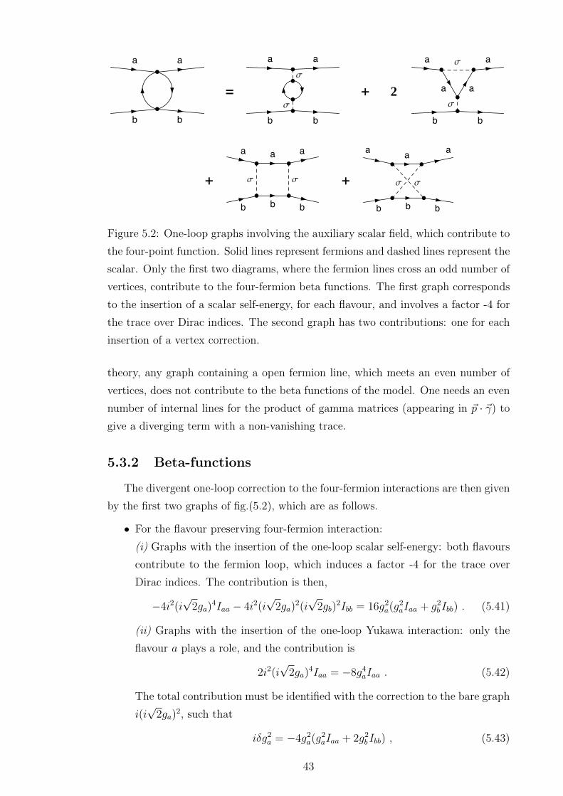
2= +

+ +

Figure 5.2: One-loop graphs involving the auxiliary scalar field, which contribute to

the four-point function. Solid lines represent fermions and dashed lines represent the

scalar. Only the first two diagrams, where the fermion lines cross an odd number of

vertices, contribute to the four-fermion beta functions. The first graph corresponds

to the insertion of a scalar self-energy, for each flavour, and involves a factor -4 for

the trace over Dirac indices. The second graph has two contributions: one for each

insertion of a vertex correction.

theory, any graph containing a open fermion line, which meets an even number of

vertices, does not contribute to the beta functions of the model. One needs an even

number of internal lines for the product of gamma matrices (appearing in ~p · ~γ) to

give a diverging term with a non-vanishing trace.

5.3.2 Beta-functions

The divergent one-loop correction to the four-fermion interactions are then given

by the first two graphs of fig.(5.2), which are as follows.

• For the flavour preserving four-fermion interaction:

(i) Graphs with the insertion of the one-loop scalar self-energy: both flavours

contribute to the fermion loop, which induces a factor -4 for the trace over

Dirac indices. The contribution is then,

−4i2(i√

2ga)4Iaa − 4i2(i

√2ga)

2(i√

2gb)2Ibb = 16g2

a(g2aIaa + g2

bIbb) . (5.41)

(ii) Graphs with the insertion of the one-loop Yukawa interaction: only the

flavour a plays a role, and the contribution is

2i2(i√

2ga)4Iaa = −8g4

aIaa . (5.42)

The total contribution must be identified with the correction to the bare graph

i(i√

2ga)2, such that

iδg2a = −4g2

a(g2aIaa + 2g2

bIbb) , (5.43)

43

and the corresponding beta function is therefore

βa ≡ Λ∂(δg2

a)

∂Λ= − g

2a

π2(g2a + 2g2

b ) . (5.44)

• For the flavour-changing interaction:

(i) Graphs with the insertion of the one-loop scalar self-energy:

16gagb(g2aIaa + g2

bIbb) ; (5.45)

(ii) Graphs with the insertion of the one-loop Yukawa interaction:

−4gbg3aIaa − 4gag

3bIbb ; (5.46)

The total contribution must be identified with the correction to the bare graph

iG

iδG = −12gagb(g2aIaa + g2

bIbb) , (5.47)

and the corresponding beta function is therefore

βG = −3gagbπ2

(g2a + g2

b ) . (5.48)

One can conclude from this one-loop analysis that the theory is asymptotically free,

since higher orders also diverge at most logarithmically, and cannot change the sign

of the one-loop beta functions. Note that, when g1 = g2, then βG = 2βa, as expected

from the O(2) symmetry.

5.4 Two-loop propagator

Since Lifshitz theories explicitly break Lorentz symmetry, space and time deriva-

tives are dressed differently by quantum corrections. As explained in chapter 2: if

one considers only one particle, or several particles in a given flavour multiplet,

frequency and space momentum can always be rescaled in such a way that the par-

ticles have the usual Lorentz-like IR dispersion relation (after neglecting the higher

order powers of the space momentum, suppressed by M). However if one considers

several particles without flavour symmetry, then it becomes necessary to perform a

flavour-independent rescaling of frequency and space momentum, such that different

particles see different effective light cones. This is the case we consider here.

The dispersion relations (5.8) are not modified at one loop, since the corresponding

graphs do not depend on the external momentum. We therefore have to go to two

loops to find the first quantum corrections, corresponding to the graphs represented

on fig.(5.3), in terms of the equivalent Yukawa model (5.39).

We note here that the two-loop propagator is evaluated in [40] for a scalar φ4 theory,

in 6 spacial dimensions and for z = 2. This calculation is done in the massless case

44

= +

Figure 5.3: Two-loop contributions to the propagator. The fermion loop in the

second graph involves a contribution from each flavour, and a factor -4 for the trace

over Dirac indices.

and in the absence of quadratic space derivatives. Dimensional regularisation is used

there, such that the power of the cut off does not appear explicitly in the results.

The authors conclude that the the Lorentz-symmetry breaking terms flow to 0 in

the deep IR.

5.4.1 Self energy

The perturbative graphs on fig. (5.3) can be calculated with massless bare prop-

agators, since the two-loop graphs contain no IR divergence. As a consequence,

these graphs are flavour independent (besides an overall factor depending on the

coupling constants), and they involve the integrals

I(k0, ~k) = i2∫dp0d

3p

(2π)4

∫dq0d

3q

(2π)4

iN(−p)iN(−q)iN(p+ q + k)

D(−p)D(−q)D(p+ q + k)(5.49)

J(k0, ~k) = i2∫dp0d

3p

(2π)4

∫dq0d

3q

(2π)4

Tr[iN(−p)iN(−q)]iN(p+ q + k)

D(−p)D(−q)D(p+ q + k),

where the trace in J arises from the fermion loop, and the factors i2 are for the

scalar propagators. Taking into account the different possibilities for the self-energy

of flavour a, we obtain

• (i√

2ga)4I for the graph without a fermion loop;

• [(i√

2ga)4 + (i

√2ga)

2(i√

2gb)2]J for the graph with a fermion loop: one contri-

bution for each flavour in the loop.

We calculate these integrals in the appendix A, where we see that the only role of

the fermion loop is to give a factor -4 from the trace over Dirac indices. We therefore

have J = −4I, and the total contribution to the momentum-dependent two-loop self

energy Σa(k0, ~k) is given by

−iΣa(k0, ~k) (5.50)

= −4g2a(3g

2a + 4g2

b )I

= −i4g2a(3g

2a + 4g2

b )

∫dp0d

3p

(2π)4

∫dq0d

3q

(2π)4

N(−p)N(−q)N(p+ q + k)

D(−p)D(−q)D(p+ q + k).

45

The bare inverse fermion propagator is

S−1bare = k0γ

0 −M2~k · ~γ + · · · , (5.51)

where dots represent higher orders in ~k. We parametrise the dressed inverse propa-

gator as

S−1dressed = −m3

a + (1− Ya)k0γ0 − (1− Za)M2~k · ~γ + · · · , (5.52)

such that the self energy is

Σa(k0, ~k) = S−1bare − S−1

dressed = m3a + Yak0γ

0 − ZaM2~k · ~γ + · · · (5.53)

The integrals (5.49) should then be expanded in the external frequency k0 and mo-

mentum ~k in order to find the corrections Ya, Za. The perturbative k-independent

mass correction m3a will be disregarded, since it is small compared to the dynamical

masses (non-analytic in the couplings) that have already been calculated nonper-

turbatively in a previous section.

5.4.2 Dressed dispersion relations

From the self energy (5.53), the IR dispersion relation for the flavour a is

(1− Ya)2k20 = m6

a +M4(1− Za)2k2 + · · · , (5.54)

where k = |~k|. If we assume that the two fermion flavours are to be coupled to other

particles, then one needs a flavour-independent rescaling of the dispersion relation.

k0 →M2k0 leads then to the following product of the phase and the group velocities,

vp and vg respectively

v2a ≡ vpvg =

k0

k

∂k0

∂k= 1 + 2(Ya − Za) +O(k/M)2 . (5.55)

We calculate Ya and Za in an appendix, A, by expanding analytically the integral I

to first order in k0 and ~k · ~γ, we find a quadratic divergence of the form (Λ >> M)

Ya − Za ' 4κ g2a(3g

2a + 4g2

b )Λ2

M2, κ ' −3.49× 10−5 (5.56)

where a 6= b. This result shows that the present model is of limited use for the

prediction of Lorentz-violating propagation. Indeed, with the values of Λ/M, g1, g2

shown in Table 1, the result (5.56) is not perturbative: one cannot then reason-

ably treat the cutoff as physical and so must absorb the quadratic divergence with

counterterms, such that the renormalised value of Ya − Za needs to be fixed by ex-

perimental data. Therefore the model cannot predict quantitative deviations from

Special Relativity at low energies.

If these corrections were logarithmic, one might be able to infer from our result

46

a cut-off-independent beta function for the effective maximum speed seen by the

fermions, which could lead to “realistic” predictions on potential sub/super-luminal

propagation.

Note that the rescaling of frequency which leads to the speed squared (5.55) does

not make apparent the fact that, if flavour symmetry is exactly satisfied, then the IR

dispersion relations are relativistic. If one ignores possible interactions with other

particles, one can further rescale

k2 = k2 1− Y1

1− Z1

1− Y2

1− Z2

, (5.57)

which leads to the following IR dispersion relations

k20 ' m2

1 + (1 + 2δv)k2

k20 ' m2

2 + (1− 2δv)k2

where δv = 6κ(g41 − g4

2)Λ2

M2. (5.58)

One can see here that the Lorentz-invariant IR dispersion relations are recovered

when g1 = g2. But for g1 6= g2, one would need the difference |g21 − g2

2| to be

proportional to M2/Λ2 in order to deal with realistic phenomenology. Taking the

largest value M/Λ ' 10−5 with ga ' 0.58 from Table 1, the upper bound δv ≤2× 10−9 given by the supernovae SN1987a data [41] gives

|g21 − g2

2| ≤δv M2/Λ2

6κ(g21 + g2

2)' 10−15 , (5.59)

such that flavour symmetry would need to be almost exact, which, if one were to

interpret as imposing h ga, could be seen as representing an unnatural fine tuning.

5.5 Conclusion

In this chapter, we have shown that flavour oscillations can be generated dynam-

ically through four-fermion interactions between (bare-)massless fermions. We have

exhibited a Lifshitz-type model in which these interactions lead to a renormalisable

theory. The IR dispersion relations of this model are significantly not Lorentz invari-

ant (in the absence of flavour symmetry): despite the altered kinematics being near

undetectable classically, quantum corrections lead to very large IR effects. Indeed,

these effects are too large for the model to be considered predictive, without a great

deal of fine tuning.

We would therefore suggest that any similar model should have logarithmic diver-

gences at worst, to be considered reasonable phenomenologically. This is the case,

for example, of Lifshitz-type Yukawa models [42], where one-loop corrections to

the fermion dispersion relations are finite. Also, Lifshitz-type extensions of gauge

47

theories, which are super-renormalisable in 3+1 dimensions and for z = 3, feature

interesting properties, see [43] and the next chapter.

It should be noted that this study treated its theory as effective, and thus its regu-

larising cut-off Λ as a possible physical constant. In the next chapter, we deal with

a model with an exact U(1) gauge symmetry, making this method of regularisation

not physically reasonable, as it does not respect the symmetries of the theory.

48

Chapter 6

Fermion effective dispersion

relation for z = 2 Lifshitz QED

This chapter is based on a paper [2], written with Jean Alexandre.

6.1 Introduction

In this chapter, we study consequences of Lorentz symmetry violation in a z = 2

Lifshitz extension of QED in 3+1 dimensions, and we again discuss the non-trivial

effects of quantisation. Because of the specific power of space momentum in prop-

agators of the model, dimensional regularisation leads to some unusual behaviour

for loop integrals, which are finite even when the space dimension goes to 3, as dis-

cussed in the appendix C. We check the consistency of the approach by calculating

the (vanishing) corrections to the photon mass and the IR-divergence-free correc-

tions to the dispersion relation for massless fermions. Our aim here is to study the

phenomenological viability of a Lifshitz QED model.

z = 2 Lifshitz QED is super-renormalisable, but still contains power counting

diverging graphs. Nevertheless, the would-be divergent graphs we calculate here

happen to be finite in 3 − ε space dimensions, after integration over frequencies,

even in the limit ε→ 0. This special feature is a consequence of the specific powers

of the momentum in this model, a phenomenon that is explained further in the

appendix C. Dimensional regularisation is still needed though, in order to define

the would-be ultraviolet (UV) diverging integrals. But because we have z = 2, the

limit ε → 0 never leads to a pole of the Gamma function and the graphs are UV

finite. The consistency of the approach is checked with the vanishing of the photon

mass correction. Divergences in scalar Lifshitz models are discussed for different

values of z and of space dimension in [44], where, in the case of scalar QED, the

effective potential for the scalar field is finite for z = 2 and in 3 space dimensions.

Another feature related to dimensional regularisation of this model is the ap-

49

pearance of poles in ε, but due to IR divergences in the case of massless fermions.

In order to calculate the integrals analytically, we will consider this massless limit,

since we are interested in the effective fermion dispersion relation, which is indepen-

dent of the mass anyway. As expected, the poles in ε generated by IR divergence

cancel each other in the calculation of the effective “maximum” speed v.

Section 2 presents the model and its properties, from which the one-loop self

energies and fermion dispersion relation are calculated in section 3, with details in

the appendix B. We eventually find that the model predicts a too important devi-

ation from IR relativistic kinematics at one-loop, if one identifies the dimensionless

coupling with the fine structure constant, whereas the classical theory is totally

justifiable in the IR regime.

A similar study has been done in [45], for a Lorentz-symmetry-violating extension

of QED - not of a Lifshitz type though - where a rescaling of fields and spacetime

coordinates, after one-loop corrections, leads to a usual relativistic IR dispersion

relation for the photon but to a subluminal propagation for fermions.

6.2 Model

We consider the following Lagrangian density for a z = 2 Lifshitz QED model,

with metric (1,-1,-1,-1),

L =1

2F0iF0i −

1

4Fij(M

2 −∆)Fij + ψ(iD0γ0 − iMDkγk −DkDk −m2)ψ (6.1)

Where Dµ = ∂µ + ieAµ and Fµν = ∂[µAν]. The mass dimensions are, in 3+1

dimensions,

[Aj] =1

2, [A0] = [ψ] =

3

2, [e] =

1

2, [M ] = [m] = 1 . (6.2)

The theory is invariant under the U(1) gauge symmetry

ψ → ψeiΛ , ψ → ψe−iΛ , Aµ → Aµ +1

e∂µΛ , (6.3)

and the classical dispersion relations are, for the photon and the fermion respectively,

k20 = M2k2 + k4

k20 = M2k2 + (k2 +m2)2 , (6.4)

where k0 denotes the frequency and k =√kiki the space momentum. After the

rescaling k0 →Mk0, the dispersion relations become

k20 = k2 +

k4

M2(photon)

k20 = m2

R + (1 + η)k2 +k4

M2(fermions), (6.5)

50

where the rescaled mass is mR ≡ m2/M and η ≡ 2m2/M2.

To get a idea of the orders of magnitude, let us consider the electron mass mR ' 0.5

MeV and the GUT scale M ' 1016 GeV. We have then m2 ' 5 × 1012 GeV2 and

η ' 10−19, which is well within the Lorentz symmetry violation bounds [7]. Also, the

corrections k4/M2 are by far currently not detectable, for energies at most k ∼ 10

TeV. For this reason, the classical model can be realistic phenomenologically. But,

as we will stress later in this chapter, quantum corrections completely change this

picture. It should also be noted that, unlike the model in the previous chapter, the

use of gauge covariant derivatives, Dµ means that the number and type of interaction

terms is dependent on the critical exponent z.

6.2.1 Propagators and interactions

The fermion propagator is given by

G(p0, p) = ip0γ0 −Mpiγi + p2 +m2

p20 −M2p2 − (m2 + p2)2

(6.6)

In order to obtain a simple photon propagator, we impose the equivalent of the

Feynman gauge condition in our anisotropic spacetime, which is

∂0A0 − (−∆ +M2)∂kAk = 0 , (6.7)

which leads to a non-local gauge-fixing term in the Lagrangian [27], but to a well-

behaved photon propagator. The gauge fixing term is

LGF = −(∂0A0 − (−∆ +M2)∂iAi)1

2(−∆ +M2)(∂0A0 − (−∆ +M2)∂jAj), (6.8)

though it can be written in a manifestly local form with auxiliary fields and is of

mass dimension 5, as required. Throughout this chapter, we shall treat the A0

and Ai lines in graphs separately, as they give different contributions; the photon

propagator is then

D00(k0, k) = −i M2 + k2

k20 −M2k2 − k4

(6.9)

Dij(k0, k) = iδij

k20 −M2k2 − k4

(6.10)

with no off-diagonal components (before quantum corrections).

There are three vertices: the 3-point ψAiψ, contributing −ie(γiM + 2p(ψ)i + p

(A)i );

the 3-point ψA0ψ, contributing ieγ0 and the 4-point AiAjψψ, contributing −2ie2δij.

From the expressions for the vertices and propagators given above, the superficial

divergence for an arbitrary graph is found to be

D = 5L− 2IA0 − 4IAi − 2Iψ +N3i , (6.11)

51

where Ix is the number of internal lines of particle x, L the number of loops and

N3i the number of three-point spacial-photon vertices. With the standard relations

L = 1 + ΣxIx−ΣaNa and (2Ix +Ex) = ΣanaNa (for each species x, where na is the

number of x-lines on the vertex a) we can re-write the above in terms of external

lines, E, as

D = 6− EAi − 2EA0 − 2Eψ − L . (6.12)

After quantum corrections we will rescale fields and coordinates such that the photon

has the usual IR relativistic dispersion relation, and we will look at the consequence

on the fermion dispersion relation. From eq.(6.12), the superficial degree of diver-

gence of the fermion propagator is 1 at one loop, such that the divergence of the

fermion wave function renormalisation is logarithmic.

6.2.2 Symmetries of the dressed propagators

As in usual QED, the polarisation tensor Πµν is transverse, since this property

arises from the structure of the source terms in the partition function and is inde-

pendent of the details of the kinetic term for the gauge field. The most general form

for Πij is, at quadratic order in the momentum,

Πij = ZM2(kikj − k2δij) +Wk20δij , (6.13)

where Z,W are dimensionless corrections to be calculated. Similarly, unitarity is

ensured by the Ward identities, which still hold as gauge invariance is unbroken.

Transversality kµΠµν = 0 implies then that the other components of the polarisation

tensor are of the form

Π0i = Wk0ki , Π00 = Wk2 , (6.14)

such that the photon dressed propagator Dµν satisfies

D−100 (k0, k) = D−1

00 (k0, k) +Wk2

D−1ij (k0, k) = D−1

ij (k0, k) + ZM2(kikj − k2δij) +Wk20δij

D−10i (k0, k) = Wk0ki .

The fermion dressed propagator is denoted, at the lowest order in momentum,

G−1(p0, p) = G−1(p0, p) + δm2 +Xp0γ0 − Y piγiM , (6.15)

where X, Y are dimensionless corrections to be calculated.

52

k k

p

k k

p+ k

−p

µ

k

k + p

k

p

µ ν

k k

p

i j

Figure 6.1: Relevant graphs for the evaluation of photon and fermion self energies.

53

6.3 One-loop propagators

The one-loop graphs contributing to the two-point functions are shown in fig.6.1;

for both fermions and photons, the graphs involving the four-point function do not

depend on the external momentum, k, and so do not contribute to the wave function

renormalisation.

6.3.1 IR behaviour

In the following sections we shall take the fermion mass to be zero, as this greatly

simplifies the calculations. This will unfortunately introduce IR divergences, which

are regularised by dimensional continuation to 3−ε spatial dimensions. Nevertheless,

as we shall show, these divergences cancel out in the calculation of corrections to

the dispersion relations.

6.3.2 UV behaviour

From naıve power counting (see eq.(6.12)), one would expect that the terms Y

and Z would be divergent (logarithmically and linearly, respectively). However,

dimensional regularisation leads to integrals of the form∫ ∞0

q2a

(q2 + q4)r−12

dq , (6.16)

(for some integers a, r), which, after dimensional continuation 2a→ 2a− ε give, for

appropriate values of ε

Γ(a− r − ε

2+ 1)

Γ(−a+ 2r + ε

2− 3

2))

2Γ(r − 1

2

) (6.17)

which can never lead to a pole of the second Gamma function in the numerator in

the limit ε→ 0, usually responsible for UV divergences. The first Gamma function

may be divergent for sufficiently high r or low a, but this is an IR divergence. To

check the consistency of this unusual feature, we show in the appendix B in section

B.1 that corrections to the photon mass indeed vanish, as expected from gauge

invariance. In the appendix C, we examine the origin of this behaviour in greater

generality.

54

6.3.3 One-loop corrections

Details of the calculations for the self energies can be found in the Appendix,

and we find

X =−e2

8π2M

(1

ε+

3

2− A

2

)+O(ε) (6.18)

Y =−e2

8π2M

(1

ε+

7

2− A

2

)+O(ε)

W =−e2

6π2M

(−1

ε− 5

3+A

2

)+O(ε)

Z =−e2

6π2M

(−1

ε+ 2 +

A

2

)+O(ε) ,

where A = γE + 2 log 2− log π and we reiterate that the poles in ε correspond to IR

divergences due to the massless fermion limit.

With the corrections calculated above, the IR kinetic terms of the one-loop dressed

Lagrangian are

LIR =1

2(1 +W )F0iF0i −

1

4(1 + Z)FijFijM

2 (6.19)

+ψ(i∂0γ0(1 +X)− iM∂kγk(1 + Y ))ψ ,

and, in order to recover the relativistic IR propagation for photons, we rescale

k0 → M(1 + Z)1/4

(1 +W )1/2k0 (6.20)

ki →1

(1 + Z)1/4ki

A0 → M1/2 (1 + Z)1/4

(1 +W )1/2A0

Ai →1

M1/2(1 + Z)1/4Ai

ψ → (1 +W )1/4

(1 +X)1/2(1 + Z)1/8ψ .

This leads to the following effective kinetic Lagrangian

M−1LeffIR = −1

4FµνF

µν + iψ

[γ0∂0 −

(1 +

δv

2

)~γ · ~∂

]ψ , (6.21)

where

δv ≡ 2Y − 2X +W − Z , (6.22)

and the factor M−1 is absorbed by the time rescaling t → Mt in the definition of

the action. As expected, the photon dispersion relation is relativistic in the IR

k20 = k2 (photon) , (6.23)

55

but the one-loop dispersion relation for fermions becomes

k20 = m2

R + (1 + δv)k2 (fermions) , (6.24)

where mR is the rescaled and dressed one-loop fermion mass, which we haven’t taken

into account up to now 1. The product of phase and group velocities for fermions is

vpvg = 1+δv, and from the expressions (6.18), we can see that the 1/ε terms cancel,

leading to

δv =1

9π2

e2

M. (6.25)

We stress again that the rescaling laws (6.20) are UV finite, and that the poles in ε

correspond to “artificial” IR divergences, as a consequence of the massless fermion

case we study here. The expected cancellation of these artificial poles in ε shows the

consistency of the definition of loop integrals, which should lead to an IR-divergence-

free expression for δv.

6.3.4 Phenomenology

If we identify the dimensionless coupling e2/M with 4πα, where α ' 1/137 is

the fine-structure constant, we obtain

δv ' 10−3 , (6.26)

which is phenomenologically not realistic. The corresponding Lorentz-violating op-

erators in the Standard Model Extension (SME) [8] are parametrised by the CPT-

even coefficients cµν , defined as

icµνψγµ∂νψ . (6.27)

In our case, we have 2cij = δv δij, such that δv = (2/3)trcij. From the tables

of SME coefficients [7], the later identification gives an upper bound of the order

|δv| . 10−15, such that one needs to consider a dimensionless coupling which satisfies

e2

4πM. 10−14 << α . (6.28)

We conclude this section with a remark concerning the dressed coupling constant

of the model. From the effective Lagrangian (6.21), gauge invariance ensures that

the IR effective interactions are

− e

M1/2ψ

[γ0A0 −

(1 +

δv

2

)~γ · ~A

]ψ , (6.29)

1Note that, since we did the calculations in the massless fermion case, the classical modification

1 → (1 + η) in eq.(6.5) is not present here. But, as explained below eq.(6.5), this contribution is

negligible compared to the present correction due to quantum effects: η << δv.

56

such that one can define the one-loop effective coupling e(1) as

e(1) ≡ e

(1 +

δv

2

). (6.30)

Although e(1) does not contain UV divergence, one can define the one-loop beta

function for the evolution of the dressed coupling e(1) with the scale M , for fixed

bare coupling e, which leads to

β ≡M∂e(1)

∂M= − 1

18π2

e3

M. (6.31)

Note that this definition of beta function does not coincide with the usual one, but

rather shows how the effective coupling of the model evolves as the crossover scale

M between Lifshitz and relativistic regimes varies.

6.4 Conclusion

We have again shown, with a specific Lifshitz extension of QED which is classi-

cally acceptable from the phenomenological point of view, that quantum corrections

change the naıve picture and lead to non-trivial Lorentz violating effects, as in the

previous chapter. In order to recover a realistic theory, the model must satisfy strong

constraints.

The U(1) gauge symmetry forced us to introduce new derivative interactions

with the UV Lifshitz scaling.

Technically speaking, it is interesting to see that, because of higher order space

derivatives, the unusual powers of space momentum lead to specific regularisation

features. Dimensional regularisation leads to a definition of loop integrals which

makes sense even in the limit where the space dimension goes to 3. The approach

is nevertheless consistent, since the physical quantities calculated here show the

appropriate cancellations of UV would-be divergences (see calculation of quantum

corrections for the photon mass) and cancellation of IR divergences in the case where

fermions are massless (see calculation of fermion dispersion relation).

We also note that taking the limit M →∞ of the present model is not straight-

forward. Indeed, since the relevant (dimensionless) coupling is e2/M , this limit

cannot be taken for fixed bare parameter e without the theory becoming trivial. For

this reason, the specific features of the present model do not allow one to continu-

ously recover usual QED in the expected way as M →∞; however, one could take

a simultaneous limit, holding the “physical” e2/M constant.

57

Chapter 7

Horava-Lifshitz gravity

7.1 Introduction

Horava-Lifshitz (HL) gravity [4] is a proposed theory of modified gravity that

appears to be perturbatively renormalisable, at least by power-counting. Though

not without its own problems, it avoids the usual problems of UV completions of

General Relativity (GR) by proposing Lifshitz scaling at high energies and exploiting

the improvements to renormalisation that the inclusion of higher derivatives brings.

As a Lifshitz theory in curved and dynamical spacetime, HL gravity is somewhat dif-

ferent to the previously examined models and thus merits a particular focus, which

is the purpose of this chapter.

We begin by introducing HL gravity in its usual form and discuss its restricted

symmetries. We then discuss the proposed extra conditions that some have applied

to HL gravity in an attempt to control the large number of possible interaction

terms it may possess and the various problems that even these proposals may fail

to cure. In the next section, we examine the linearised classical behaviour of HL

gravity, demonstrating the “extra” scalar degree of freedom. We then examine the

“covariant” extension of HL gravity that will be the focus of the next chapter. Fi-

nally, we relate HL gravity to other popular deformations of GR.

For recent reviews of HL gravity, see [46] [47] [48].

Metric conventions

As this is a proposed ultraviolet completion to General Relativity, we shall adopt

the mostly-plus metric convention generally used in studies of general relativity, so

that what we present may be more readily compared with the existing literature. We

emphasise that this is the opposite convention to that used in the preceding chapters.

58

7.2 Model

In HL gravity, where we shall take z = d = 3, it is natural to take the ADM

form of the space-time metric:

ds2 = −c2N2dt2 + gij(dxi +N idt

) (dxj +N jdt

), (7.1)

where c is the speed of light, with dimension [c] = 2. The gravitational degrees

of freedom are the lapse function N(x, t), the shift function Ni(x, t) and the 3-

dimensional space metric gij(x, t). The mass dimensions of metric components are

[N ] = 0, [Ni] = 2, and [gij] = 0.

We relax the assumption of local diffeomorphism invariance

xµ → x′µ(xν) (7.2)

to allow z = 3 Lifshitz scaling in the ultraviolet; this forces us to distinguish a time

co-ordinate and space directions at each point, producing a foliation of the space

time, the leaves of which are surfaces of constant time (and so giving a global notion

of simultaneity). The symmetry group is now restricted to the foliation-preserving

diffeomorphisms

xi → x′i(xj, t), t→ t′(t). (7.3)

Perturbatively, these transformations can be represented by:

δt = f(t) (7.4)

δxi = ξi(t, x)

δgij = ∂iξj + ∂jξi + ξk∂kgij + fgij

δNi = ∂iξkNk + ξk∂kNi + ξjgij + fNi + fNi

δN = ξk∂kN + fN + fN .

A generic action for HL gravity can be given by

S =1

ε2

∫dtd3x

√gNKijK

ij − λK2 − V

(7.5)

Where

Kij =1

2Ngij −∇iNj −∇jNi , i, j = 1, 2, 3 (7.6)

is the extrinsic curvature (with K = Kii), λ a dimensionless constant, ε a coupling

constant determining the strength of gravity (analogous to Newton’s constant G in

general relativity), g the determinant of the space metric.

59

V is an arbitrary potential made from foliation-preserving-diffeomorphism-invariant

terms containing up to 6 space derivatives of the metric. There are no such invariant

terms one can construct from Ni or time derivatives of N , so one need only consider

the various contractions of derivatives, the 3-space Ricci tensor Rij and the accel-

eration vector ai = ∂i lnN (the Riemann tensor can be expressed in terms of the

Ricci tensor in 3 dimensions). It should be noted that the term aiai is of the same

mass dimension as the R expected from General Relativity.

If the potential is allowed to contain 6-derivative terms, such as R∆R (where R

is the 3-dimensional Ricci scalar of the leaves of the foliation), then the theory is

power-counting renormalisable [4]. (Indeed, as gij is dimensionless, all its couplings

for interactions with up to six derivatives should be marginal or relevant). The con-

dition z = d was not arbitrary, such a choice makes the coupling ε (or equivalently,

Newton’s G) marginal.

The action for General Relativity can be recovered in the case where λ = 1 and

V = −Λ− c2R. Note then, that there are two separate sources of Lorentz violation

in this model: the higher order terms in the potential, which classically should only

have noticeable effects at very high energies, and the possibilities that λ 6= 1 or that

aiai has a non-vanishing coupling, which (classically) suffer no such suppression in

the IR.

7.3 Restrictions

As there are a great number of terms that could appear in the potential, two

restrictions have been proposed by Horava:

7.3.1 Detailed Balance

Detailed balance is the suggestion that the potential should be given by

V = EijGijklEkl (7.7)

where

Gijkl =1

2(gikgjl + gilgjk)− λgijgkl

√gEij =

δW [g]

δgij(7.8)

for some action W . This restriction was inspired by HL gravity’s origins in con-

densed matter and critical phenomena, but does not seem a very sensible restriction

60

for models in which Lorentz violation is imposed “by hand” and so shall not be

considered further. Indeed, it has been found to lead to additional problems beyond

those of HL gravity in general [49], such as a wrong-sign cosmological constant (for

reasonable values of λ). The detailed balance condition also necessarily introduces

parity violating terms to the action.

7.3.2 Projectability

Projectability (and hence “Projectable Horava-Lifshitz gravity”) is the proposal

that the lapse function, N , be a function of time only. Such a condition is preserved

under the foliation-preserving diffeomorphisms, as ξk∂kN vanishes, and removes any

terms containing spatial derivatives of N(t) from the potential, leaving it a function

of the 3-dimensional intrinsic curvature alone. Many important solutions in GR

have a natural co-ordinate system in which this condition is true (for example:

the various black hole solutions, FRWL cosmology) and it could of course always

be imposed, so it does not seem too unreasonable to apply the same to HL gravity.

With this condition, the number of terms in the potential becomes more manageable;

if we further restrict our potential to not violate parity (as we could by including a

term constructed from the Cotton tensor) there are only nine possible terms in the

potential that can be expressed as

Vproj = −Λ− c2R− α1R2 − α2RijR

ij − β1R3 − β2RRijR

ij

− β3RjiR

kjR

ik − β4R∆R− β5∇iRjk∇iRjk, (7.9)

where all other contractions can be related to those above by some identity or an

integration by parts [47]. However, the ai terms that we have excluded here have

been used to improve the IR behaviour of some Horava gravity models [50], and

can be used to reproduce MOND phenomenology (see section 7.8). Additionally, as

we now have a field that depends on time only, its variation leads to a Hamiltonian

constraint integrated over space, which can complicate Hamiltonian analyses of HL

models. The extra scalar degree of freedom discussed below also appears to be

unstable in projectable HL gravity, having the “wrong” sign for its low-energy kinetic

terms.

7.4 Problems

7.4.1 Scalar graviton

Having removed one generator of local symmetries, it is not surprising that HL

gravity contains one additional propagating degree of freedom per space-time point

61

when compared with general relativity, normally referred to as a “scalar graviton”.

We can see this by counting the degrees of freedom by the Hamiltonian method

given in [51]: the number of primary constraints to take into account is the number

of gauge functions plus the number of their time derivatives, in the situation where

these gauge functions depend on both space and time. This is because gauge func-

tions and their time derivatives must be considered independent, when defining a

boundary condition for the evolution of gauge fields. In our case (not assuming pro-

jectability), we have 10 independent metric components (N, Ni, gij) and we see from

the gauge transformations (7.4) that the functions ξi count twice since they appear

with their time derivative, while f counts once only because it depends on t only.

The total number of propagating degrees of freedom is therefore 10−(2×3+1) = 3,

consistent with the loss of one generator of symmetry.

This extra mode is problematic in that it does not generically decouple at low

energies, and so it becomes difficult to recover GR in the infra-red, where the per-

turbative approximation to GR is very well tested. Indeed, it appears to become

strongly coupled at low energies [49] at a scale around

Mstrong ∼Mpl

√|1− λ| , (7.10)

or even lower [52], which is a problem when λ ∼ 1 is the limit one might hope to

reach in the IR and is strongly constrained by experiment.

In [52], the simultaneous limit where Mpl →∞ while Mstrong (and its equivalent

from aiai) remains constant is investigated, it is found that strong coupling still

generally occurs, at a lower mass scale.

Several methods have been proposed to solve this problem: [50] suggests that a

non-projectable HL gravity with non-zero couplings to several of the ai terms may

remove the issue, but the couplings must be quite large.

It should be noted that this term does not appear at the relativistic value of

λ = 1, where its kinetic term vanishes; many attempts to cure this problem try to

force the theory to flow to this point in the IR (but these encounter the issues of

strong coupling mentioned above). Indeed, if one considers the lowest dimension

terms in the Lagrangian

L =√gN [KijKij − λK2 + c2R + αaia

i + . . .] (7.11)

and performs an expansion about flat space, one finds (after fixing the gauge and

applying the linearised classical equations of motion for the non-propagating fields,

see the next section for details), two distinct propagating species:

• A spin 2 graviton, as found in GR, with propagation speed c (taken to be 1

by rescaling).

62

• The spin 0 graviton, with propagation speed

c20 =

1− λ3λ− 1

.α− 2

α(7.12)

from which we can obtain the condition that, for the spin 0 graviton to behave

sensibly (that is 0 < c20 < 1) we require

0 < α < 2,

λ > 1 or λ <1

3(7.13)

(the other sign for α is disallowed as it would give the wrong sign to a time derivative

term in the action. Projectability, of course, would impose α → ∞, but this speed

is derived from two separate terms in the expansion, one of which does not appear

in the projectable case as we shall see in the next section).

It has also been argued that flowing to the fixed point at λ = 1/3 can be used

to remove the unwanted scalar [53], but the region between that and the relativistic

λ = 1 is disallowed by the above.

7.4.2 Quantisation and interactions

HL gravity, by naturally providing a foliation of spacetime, removes one of the

difficulties in consistently quantising gravity theories, the seemingly arbitrary choice

of time co-ordinate under which ones quantised theory may not be invariant. Be-

cause of this, most attempts at quantisation of this model have followed simple

canonical formalisms. However, many of the problems of quantising theories of dy-

namical spacetime remain, and several of the methods developed for GR have been

applied to HL gravity.

We note here related works, involving the quantisation of HL gravity. [54] shows

that in the large N limit of projectable HL gravity, coupled to N Lifshitz scalars, the

matter-induced beta functions display asymptotic freedom. Exact Renormalisation

Group methods are used to provide an insight into the existence of asymptotically

safe gravity [55], in that the IR relevant terms of projectable HL gravity flow to

a non-gaussian fixed point in the UV (also of note in the same model is that the

Einstein-Hilbert action is a saddle point with an IR-attractive direction).

Also, [56] is based on causal dynamical triangulations to study phase transitions

of space time geometry in (2+1)-dimensional HL gravity. Finally, [57] describes

how (1+1)-dimensional HL gravity can be quantised in a similar way as a harmonic

oscillator.

63

There is not a unique way of coupling HL gravity to matter that may be Lifshitz-

scaling itself, as one may include higher derivative terms in the matter sector also,

but there do exist minimal consistent couplings for several models [58], [59].

In [60], the authors derive a general coupling to non-projectable HL gravity for

scalars and vectors and then evaluate low-order propagation corrections in a manner

similar to the two proceeding chapters. Interestingly, the authors find that higher

derivative terms are generated dynamically even for “relativistic” matter.

7.5 Expansion about flat space

To explicitly demonstrate the classical behaviour we have discussed above, we

shall now derive the linearised equations of motion for HL gravity about flat space.

We shall assume projectability, as that is the most relevant case to our subsequent

work.

L =√gN(t)[KijKij − λK2 − V ] (7.14)

7.5.1 Constraints

Varying the action with respect to N(t) yields the Hamiltonian constraint∫d3x√g(KijKij − λK2 + V ) = 0 (7.15)

integrated over spatial slices as N is a function of t only. Varying the shift vectors

Ni gives the supermomentum constraint

∂i(Kij − λKgij) = 0 . (7.16)

7.5.2 Gauge fixing

We chose the synchronous gauge N = 1, Ni = 0 and expand the spatial metric

about flat space as gij = δij + εhij. Our supermomentum constraint now reads (to

lowest order)

∂t∂i[hij − λhδij] = 0 +O(ε) (7.17)

which implies ∂i[hij − λhδij] = vj(x). for some vector vi a function of space only.

We still have a residual gauge transformation not fixed by the conditions above:

hij → hij + ∂iuj(x) + ∂jui(x) (7.18)

which can be used to set vi = 0 (if λ 6= 1) and so remove the vector part of hij. We

can now decompose hij into a scalar part h and a traceless, transverse tensor part

Hij by defining the transverse tensor

Cij = hij − λhδij (7.19)

64

and letting Hij = Cij − 13δijCkk be the trace-free part of Cij. We now have

hij = Hij −3λ− 1

2(δij −

∂i∂j∂2

)h+ (1− λ)δijh. (7.20)

7.5.3 Equations of motion

Now, the linearised equation of motion reads

1

2∂2t [hij − (1− λ)δijh] = Vij +O(ε) (7.21)

where Vij is a functional derivative of the potential with respect to hij. This can be

easily split into the two components above by taking a trace:

(1− 3λ)∂2t h = −2Vkk

∂2tHij = 2Vij − (δij −

∂i∂j∂2

)Vkk. (7.22)

If we take V = −R, we obtain

∂2tHij = ∂k∂kHij +O(ε),

(1− 3λ)∂2t h = (1− λ)∂k∂kh+O(ε) (7.23)

almost recovering the dispersion relations from the previous section; although, as

mentioned, the sign of c20 is incorrect, an additional problem for the scalar graviton

in the projectable case.

7.6 Cosmological bounds

A recent study [61] considered HL gravity in the context of effective field theories

for modified gravity and dark energy. From this, perturbative cosmological and

astrophysical predictions could be derived with standard computational packages

and compared to known experimental measurements. The most strongly constrained

parameters are of course those of the lowest dimension terms in the HL gravity

Lagrangian, i.e.

LIR =√gN [KijKij − λK2 + c2R + αaia

i] (7.24)

Comparatively strict bounds are found on λ and α:

|1− λ| < 10−6.2

α < 10−2.4 (7.25)

Because of higher-order corrections we have not considered elsewhere in this chapter,

c2 is not expected to be exactly the relativistic speed of light, and so we have the

additional bound |c2 − 1| < 0.0038.

We additionally note that if the parameters are tuned so that the Post-Newtonian

parameters used in solar system tests vanish exactly, the constraint on α becomes

as stringent as that on λ.

65

7.7 Covariant Horava-Lifshitz gravity

An interesting solution to the problem of the extra scalar was proposed in [62],

in which an extra U(1) gauge symmetry is introduced to restore a modified form of

“covariance” and so bring the number of propagating degrees of freedom back to its

relativistic value.

7.7.1 Symmetries and Lagrangian

We introduce an extra local symmetry by first noting that the transformation

generated by δNi = ∂ia for some scalar a is a symmetry of linearised Horava gravity

(about flat space). To close the symmetry in the full theory, we must introduce

• an auxiliary scalar field ν

• a field A that acts as a Lagrange multiplier and transforms as a vector under

time reparametrisations but as a scalar under spatial transformations (i.e like

N),

leading to an action of the form 1

S =1

ε2

∫dtd3x

√gN[KijK

ij − λK2 − V + νΘij(2Kij +∇i∇jν)]− A(R− 2Ω)

,

(7.26)

where

Θij = Rij − 1

2Rgij + Ωgij (7.27)

and Ω is a constant. Under the new U(1) symmetry the ν, A and Ni fields transform

as

δαNi = N∇iα

δαA = α−N i∇iα

δαν = α (7.28)

and all others are invariant. Note that [A] = 4, [ν] = 1.

7.7.2 Degree of freedom counting

By a simple extension of the degree of freedom counting argument given for nor-

mal HL gravity above, we can see that this theory will indeed possess only the two

propagating degrees of freedom that we require (as we have introduced two extra

constraints at the cost of one extra scalar).

1It has been shown in [58] that the present extension to the original HL gravity is valid for any

λ, despite its original derivation at λ = 1.

66

Alternatively, it could be noted that the Lagrange multiplier A imposes a con-

stant value of R = 2Ω. This introduces an additional constraint to the calculations

in section 7.5 (to be exact, a constant value for ∂2h) which indeed removes the scalar

“trace” degree of freedom. (The extra scalar d.o.f. introduced with the auxiliary

field is removed by gauge fixing.)

7.7.3 Problems

The aforementioned fixing of the value of R (i.e. the intrinsic curvature of the

leaves of the preferred foliation) by the Lagrange multiplier is not problematic in a

pure gravity scenario but may be considered inconsistent in the presence of matter,

but this is neglecting the possibility that the “dressed” curvature may differ signifi-

cantly from what we have calculated here, once all possible interactions with matter

are considered (including couplings between matter fields and A).

We note that the long-distance IR limit is not obviously recovered: it has been

shown in [63] that the equivalence principle is not automatically retrieved in the

infra-red. The meanings of the auxiliary fields and their couplings to matter are

still open questions, though the field ν is sometimes known as the “prepotential”

as its divergence contributes to the Newtonian gravitational potential. It has been

shown [64] that in the projectable case, one can recover seemingly relativistic IR

behaviour by taking the A and ν fields to be part of the effective 4-metric for matter

(in the non-projectable case, no such assumption is needed [65]).

7.7.4 Other work

This covariant extension to HL has led to several studies, including spherically

symmetric solutions [66] and their relevance to an alternative model for galaxy rota-

tion curves [67], cosmological solutions [68], as well as theoretical and phenomeno-

logical consistency tests of the theory [69].

This version of HL gravity will be discussed further in Chapter 8.

7.8 Relating HL gravity to other modified gravity

models

7.8.1 Einstein-Aether and khronometric models

One of the simpler Lorentz violating modifications to General Relativity that

has been considered is Einstein-Aether theory: we introduce a vector field uµ, the

“aether”, restricted to be time-like and of unit length (i.e. uµuµ = −1, usually

67

imposed by a Lagrange multiplier). The most general coupling, in the IR can be

given by

SEA =1

16πG

∫d3xdt

√g(R +∇µuν∇ξuρ(c1g

µξgνρ + c2gµνgξρ + c3g

µρgνξ + c4uµuξgνρ)

+ λ(uµuµ + 1))

(7.29)

Where the ci are constants and λ is a Lagrange multiplier. Although this action is

still “covariant” in that it is defined in terms of 4-tensors, clearly the presence of

uµ explicitly breaks Lorentz symmetry and we have a preferred local rest frame in

which u = (1, 0, 0, 0).

This is a very general model of low-energy Lorentz violation in the gravity sector,

in order to relate it to HL gravity, we must consider a specific case: the “khronomet-

ric” model, in which uµ is additionally assumed to be the gradient of some scalar τ

(the “khronon”);

uµ =∇µτ√|∇ντ∇ντ |

(7.30)

suitably normalised to be of unit length. One can see that the sets of constant τ

must be 3-dimensional everywhere (so that uµ 6= 0), providing a foliation of our

spacetime; additionally, uµ is unchanged by a reparametrisation τ → τ ′(τ).

Moving to ADM co-ordinates respecting this foliation, we can identify

N =1√∇ντ∇ντ

g(3)ij = gij + uiuj

Kij = ∇iuj (7.31)

We can then see that the interaction terms in 7.29 are reduced to those that preserve

the foliation, eg.

∇µuν∇µuν = KµνKµν − a2 (7.32)

all of which are some combination of R,K2, KijKij and aia

i; the same relevant IR

terms as are possible in HL gravity, so we conclude that khronometric and (non-

projectable) Horava models have the same low-energy classical behaviour.

7.8.2 Dark matter free models

The continued non-observation of a dark matter candidate has led some to pro-

pose modifications to gravity to explain the observed galaxy rotation curves.

MOND

MOND (MOdified Newtonian Dynamics) posits an infra-red modification to

gravitational physics: a dependence on an acceleration scale that can be used to

68

explain (some of) the phenomena usually attributed to dark matter. MOND ac-

quires its name from the way it can be treated as a modification to the Poisson

equation for Newtonian gravity:

∇.(f(|∇φ|a0

)∇φ) = 4πGρ (7.33)

where a0 is the acceleration scale, and f is a function such that f(x)→ 1 as x→∞and f(x) ∼ x as x → 0. It can be shown [70], [71] that a model with a suitable

function of the acceleration vector ai in the potential can reproduce this behaviour.

We can thus recover MOND at low accelerations with both khronometric and non-

projectable HL gravity models.

Galaxy rotation curves from projectable, covariant Horava-Lifshitz grav-

ity

In [67] the authors attempt to emulate dark matter through an appropriate choice

of the covariant HL auxiliary field A in a projectable covariant Horava-Lifshitz model

(similar to the one we shall study in the next chapter). They consider the spherically

symmetric solution

ds2 = −c2N2dt2 +1

f(r)(dr + n(r)dt)2 + r2dΩ (7.34)

where n(r) is the radial component of the shift vector Ni. Taking λ = 1 (as must

be approximately true), they examine the classical equations of motion, from the A

and n equations, they find

n∂rf = 0

f = 1− B

r(7.35)

for some constant B. This implies either B or n vanishes; taking n 6= 0 and gauge

fixing ν = 0, the remaining equations of motion (which we shall not repeat here)

lead to multiple solutions for n,A, given by

n2 =c

r− 1

2A(r) +

1

2r

∫ r

0

A(ρ)dρ ,∫ ∞0

A′(r)dr = 0 (7.36)

The reason one finds multiple solutions here is that the Hamiltonian constraint is

integrated over space, as we are considering the projectable form of covariant HL

gravity here.

69

The authors then attempt to recover observed galaxy rotation curves: first they

set A = 0 outside the virial radius of the galaxy, as a boundary condition. Consid-

ering the Newton potential from these fields alone, one finds

φ(r) =−n2

2c2(7.37)

Thus, to recover any given orbital velocity profile v(r) inside the galaxy, one requires

1

4c2rA′(r) = v2(r) +

∫ r

0

dρv2(ρ)

ρ(7.38)

which indeed has consistent solutions for physically reasonable choices of v.

It should be noted that a non-vanishing A also contributes to the vacuum energy

of the universe, but this can be put within experimental bounds.

This example can be considered a clear demonstration that projectable covariant

HL gravity does not necessarily recover GR at low energies, at least without a careful

choice of parameters. This is discussed further in[64].

70

Chapter 8

Effective matter dispersion

relation in quantum

covariant Horava-Lifshitz gravity

This chapter is based on a paper [3], written with Jean Alexandre.

8.1 Introduction

In this chapter, we study the effective dispersion relations of classical matter

fields (a complex scalar and a photon) coupled to the covariant extension of pro-

jectable Horava-Lifshitz gravity introduced last chapter in section 7.7. The fields are

“classical” in that we treat them as external sources and integrate over the gravity

degrees of freedom only, to one loop, about a flat background metric.

In this case, we take the coupling Ω = 0, such that the constraint provided by

the auxiliary field A consists of setting the curvature tensor to zero, R = 0, which we

impose in the path integral over metric fluctuations. The restoring force for quantum

fluctuations is then provided by higher order space derivatives of the metric, and

leads to a prediction for the Lorentz-symmetry violating effective dispersion relations

for these fields.

Because the matter fields are classical, the present model contains only logarith-

mic divergences. Additionally, our results suggest that the characteristic Horava-

Lifshitz scale should be smaller than 1010 GeV, if one wishes not to violate the

current bounds on Lorentz symmetry violation.

The effective speed of light seen by matter interacting with HL gravity is studied

71

in [72]. The authors derive this effective speed seen by a scalar field and an Abelian

gauge field, and compare these to measure Lorentz-symmetry violation in a similar

manner to the present study. However, we are treating matter as classical, and

imposing the constraint R = 0 in the integration over graviton degrees of freedom.

We emphasise that R = 0 is not a gauge choice, but a constraint from the additional

symmetry of our model which has the physical effect of removing one degree of

freedom in the theory. As described below, the constraint leads to the vanishing of

one of the scalar components of the space metric.

Similarly, in [60], effective dispersion relations are calculated for “relativistic”

scalars minimally coupled to conventional non-projectable HL gravity; it is found

that higher-derivative terms for the scalars are dynamically generated, as might be

expected generically.

A short review on the covariant version of HL gravity is presented in the next

section, and the coupling to matter fields is presented in section 3, together with the

integration of gravitons. This calculation is done for λ 6= 1, but the result does not

depend on λ, which is a consequence of the vanishing of the trace of the fluctuating

space metric. Section 4 presents a phenomenological analysis and our conclusions.

8.2 Review of covariant Horava-Lifshitz gravity

Although it was previously described in section 7.7 we present a condensed in-

troduction to Covariant HL gravity here.

8.2.1 Notation

Recall our convention that tensors with repeated lower indices are contracted

with the flat space metric, and that

viwi = viwjgij = (g−1

ab )ijviwj . (8.1)

Also, we denote v2 = vivi, we use ∂i for the flat 3-space derivative, and ∂2 for the

flat 3-space Laplacian.

We repeat again here that we use the “mostly plus” metric signature convention

in this chapter.

8.2.2 The action

We consider the z = d = 3, projectable, covariant HL gravity. The gravitational

degrees of freedom are the lapse function N(t), the shift function Ni(x, t) and the 3-

dimensional space metric gij(x, t), which appear in the ADM form of the space-time

72

metric 7.1. c is the speed of light, with dimension [c] = 2. The mass dimensions of

metric components are [N ] = 0, [Ni] = 2, and [gij] = 0.

The covariant version of HL gravity involves the auxiliary gauge fields A(x, t)

and ν(x, t) whose role is to impose a constraint which eliminates the scalar degree

of freedom of HL gravity. The action is then given by

S =1

ε2

∫dtd3x

√gN[KijK

ij − λK2 − V + νΘij(2Kij +∇i∇jν)]− AR

, (8.2)

where

Kij =1

2Ngij −∇iNj −∇jNi , i, j = 1, 2, 3 (8.3)

Θij = Rij − 1

2Rgij

V = −c2R− α1R2 − α2R

ijRij − β1R3 − β2RR

ijRij

−β3RjiR

kjR

ik − β4R∇2R− β5∇iRjk∇iRjk .

Note that [A] = 4, [ν] = 1, [ε] = 0, the potential V includes all the renormalisable

operators even under parity and we have taken the parameter Ω = 0. The dimensions

of the various terms in the Lagrangian are

[R] = 2, [R2] = 4, [R3] = [∆R2] = 6, [c2] = 4, [αi] = 2, [βj] = 0 . (8.4)

Note that the term RijklRijkl does not appear, as the Weyl tensor in three dimen-

sions automatically vanishes.

The action (8.2) is invariant under the following transformations:

• 3-dimensional foliation-preserving diffeomorphism

δt = f(t) (8.5)

δxi = ξi(t, x)

δgij = ∂iξj + ∂jξi + ξk∂kgij + fgij

δNi = ∂iξkNk + ξk∂kNi + ξjgij + fNi + fNi

δN = ξk∂kN + fN + fN

δA = ξk∂kA+ fA+ fA

• U(1) symmetry

δαN = 0

δαgij = 0

δαNi = N∇iα

δαA = α−N i∇iα

δαν = α (8.6)

where α is an arbitrary spacetime function.

73

8.2.3 Gauge fixing and U(1)-symmetry constraints

The metric fluctuations hij are defined by gij = δij + εhij and, choosing the

synchronous gauge where N = 1 and Ni = 0, we decompose hij as

hij = Hij + ∂iVj + ∂jVi + (1

3δij −

∂i∂j∆

)B +1

3δijh, (8.7)

where Hij is transverse traceless, Vi is transverse and h =trhij.One can easily see that the variation of the action (8.2) with respect to A leads

to R = 0, which is a condition we will impose in the path integral over graviton

degrees of freedom. This condition should be satisfied at the linear order in met-

ric fluctuations, since we consider only quadratic terms in the gravity action. We

therefore obtain

0 = R = −ε23∂2(B + h) +O(ε2) , (8.8)

which, together with boundary conditions h(∞) = B(∞) = 0 leads to h = −Beverywhere. We can re-write our expansion of hij as

hij = Hij + ∂iVj + ∂jVi +∂i∂j∆

h. (8.9)

Finally, We fix the U(1) symmetry by setting ν = 0, and we also note that

ghosts decouple from matter at one loop, since the corresponding action is cubic in

fluctuations of ghosts/gravitons.

8.3 Effective dispersion relation for matter fields

8.3.1 Coupling to matter

We now wish to couple the gravity sector to classical matter, including a complex

scalar field φ and an abelian gauge field Aµ. In [58] a generic action is derived for

the coupling of Covariant HL gravity to a scalar field, but we restrict ourselves to

the case which recovers Lorentz symmetry in the IR

Sscalar = −∫d3xdt

√g(−φφ? + c2gij∂iφ∂jφ

?) , (8.10)

where c is the speed of light, with mass dimension 2.

The coupling to an abelian gauge field Aµ is described by the action

Sphoton = −1

4

∫d3xdt

√g(−2gijF0iF0j + c2gikgjlFijFkl) , (8.11)

and we need not worry about gauge fixing for the abelian field Aµ, since it is con-

sidered an external source. We wish to calculate effective dispersion relations for

the matter fields φ and Aµ. As these fields couple to gravity only through their first

derivatives, we may treat those derivatives as constant external fields:

74

• φ = φ0 exp(ikµxµ) leads to ∂iφ∂iφ? = (~k)2φ2

0;

• Ai = A0i sin(kµxµ) leads to F 2

ij = 2(~k)2(A0)2 − 2(~k · ~A0)2 +O(k4).

The (anisotropic) effective action will be given by an expression of the form

Seffscalar =

∫d3xdt((1 + a)φφ? − (1 + b)c2∂iφ∂iφ

?) , (8.12)

with a corresponding dispersion relation

(1 + a)k20 = (1 + b)c2k2 , (8.13)

where we assuming a, b 1. If we note v2φ the product (phase velocity × group

velocity), we have thenv2φ

c2− 1 = b− a+O(ε3) (8.14)

Similarly, for the photon we will obtain an effective action of the form

Seffphoton = −1

4

∫d3xdt(−2(1 + a′)F0iF0i + c2(1 + b′)FijFij) , (8.15)

with the corresponding correction

v2A

c2− 1 = b′ − a′ +O(ε3) . (8.16)

As noted in [72], the measurable quantity which violates Lorentz symmetry is the

difference

δv2 ≡ |v2A − v2

φ| = c2|b′ − b− a′ + a| . (8.17)

8.3.2 Features of the one-loop integration

Taking into account the above gauge fixing conditions and the constraint R = 0

in the path integral, the gravity sector expanded to second order in the metric

fluctuations reads

Sgravity = −1

4

∫d3xdt Hij(x)

(∂2t + 4α2∂

4 − 4β5∂6)Hij

+ 2∂iVj∂2t ∂iVj + (1− λ)h∂2

t h+O(ε) (8.18)

Note that only the terms from the potential with no powers of R survive, and only

those with two powers of Rij contribute at this level, as Rij is O(ε). We can now

see that we have only two propagating degrees of freedom (the two polarisations of

Hij), as expected.

As the remaining two components of the metric, Vi and h, have only time deriva-

tives, one may suspect that the theory would be unstable. This is not believed to be

75

the case; instead, this scenario is analogous to the “conformal instability” of pertur-

bative GR. The conformal instability can be seen if one makes a naıve decomposition

of the metric perturbations into trace and trace-free parts: the kinetic term for the

trace component in the Lagrangian has the wrong sign. However, careful consid-

eration of the Jacobian factors [73] reveals that the trace term is non-propagating

(which is obvious in our case) and can be re-interpreted as an auxiliary field imposing

an additional constraint (but only after a non-local change of co-ordinates).

Indeed, in [74] similar calculations to our own are performed “on-shell” in non-

projectable HL gravity (and another Lorentz-violating model) by treating the non-

propagating fields as auxiliary and imposing their equations of motion as constraints

in the path integral. The authors find results not dissimilar to those we shall derive

shortly. A similar strategy could have been adopted here; however, the constrained

action would be non-local (as the auxiliary fields appear with mixed orders of deriva-

tives, taking their interactions with the matter fields into account) and more difficult

to work with.

We may treat the cases of photons and scalars separately at the order at which

we are working, as they have no interactions other than through gravity.

For the scalar we have

Sscalar =

∫d3xdt

Lφ0 + ε2c2

(− 1

3HijHij −

2

3∂iVj∂iVj −

1

6h2

)∂kφ∂kφ

? +O(ε3)

(8.19)

where Lφ0 is proportional to − ˙|φ|2 + c2∂iφ∂iφ?, the usual relativistic Lagrangian

density for the scalar. Following [72], because of isotropy in space coordinates,

terms of the form T ij∂iφ∂jφ? that are quadratic in the graviton fields have been

replaced by (1/3)T ii ∂jφ∂jφ?. Terms that mix different components of the graviton

cannot contribute to our corrections at O(ε2) and so are neglected here. Terms

linear in the graviton fields do not contribute here either, as we treat the scalars as

classical external fields; for the same reason, we are able to integrate the quadratic

terms by parts.

Similarly, for the photon we have

Sphoton =1

4

∫d3xdt

LA0 + ε2c2

(− 1

6HijHij −

1

3∂iVj∂iVj −

1

6h2

)FklFkl +O(ε3)

,

(8.20)

where isotropy has been used and LA0 is proportional to the relativistic Lagrangian

for photons.

76

8.3.3 Integration

As the components of the graviton do not mix, we may consider their contribu-

tions separately.

Spin 2

As we seek the difference between the modifications to the space and time com-

ponents, we can neglect in the action the term Lφ0. We therefore need only to

consider the action

Sscalar = −1

4

∫d3xdt Hij(x)

(∂2t + 4α2∂

4 − 4β5∂6 +

4ε2

3c2∂kφ∂kφ

?

)Hij(x) .

(8.21)

for the scalar and

Sphoton = −1

4

∫d3xdt Hij(x)

(∂2t + 4α2∂

4 − 4β5∂6 +

2ε2

3c2 1

4FklFkl

)Hij(x) .

(8.22)

for the photon.

Scalar field

We denote by D(q) the Fourier transform of ∂2t + 4α2∂

4 − 4β5∂6 , and we have

SH = −1

4

∫d3pdp0

(2π)4

d3qdq0

(2π)4Hij(p)

(D(q) +

4ε2

3c2∂kφ∂kφ

?

)δ(p+ q) Hij(q) . (8.23)

Integrating over the two components of H, this gives a contribution to the partition

function of (Det

(D(q) +

4ε2

3c2∂kφ∂kφ

?)δ(p+ q)

)−1

(8.24)

= exp

−Tr

[ln (D(q)δ(p+ q)) +

4ε2

3c2∂kφ∂kφ

? D−1(q)δ(p+ q)

]= exp

−4ε2

3c2∂kφ∂kφ

?δ(0)

∫d3pdp0

(2π)4

1

−p20 + 4α2p4 + 4β5p6

+ · · ·,

where δ(0) is a constant global volume factor, and dots represent field-independent

terms. The integral in the above leads to:

I = −δ(0)4ε2

3c2∂kφ∂kφ

?

∫d3pdp0

(2π)4

1

−p20 + 4α2p4 + 4β5p6

= −δ(0)4ε2

3(2π)4c2∂kφ∂kφ

? × −iπ2

∫d3p

p2√α2 + β5p2

, (8.25)

and is logarithmically divergent. We regularise this integral by dimensional regular-

isation, as it respects the symmetries of the theory

Ia = −δ(0)4ε2

3(2π)4c2∂kφ∂kφ

? × −iπ2

∫(3− a)π

3−a2 p2−adp

Γ(5−a2

)p2√α2 + β5p2

µa

= iδ(0)ε2

6π2c2∂kφ∂kφ

? 1√β5

µa

a+ finite , (8.26)

77

where µ is an arbitrary mass scale. After dividing by iδ(0), in order to take into

account the Wick rotation and the space time volume, the identification with the

speed (8.14) givesv2φ

c2− 1 =

−ε26π2√β5

µa

a. (8.27)

Photon

Comparing the coefficients of the relevant terms in the actions, one can see the

effective change in velocity for the photon will be 1/2 times that of the scalar. This

leads tov2A

c2− 1 =

−ε212π2√β5

µa

a. (8.28)

Note that both these results are sub-luminal, as might intuitively be expected: small

fluctuations of the spatial metric about flat space should generally lead to a “longer”

path between two points.

Spin 1

The spin 1 terms are similar to the spin 2 terms shown above, with 2∂iVi∂iVi in

the place of HijHij. However, the calculation leads to an integral of the form∫d3pdp0

(2π)4

1

p20

. (8.29)

Unlike the previous case, the p integral here is the integral of a polynomial, which

can be formally taken to vanish under dimensional regularisation, as explained in

appendix C (see also [75]). The vanishing or finiteness of a regularised integral

which otherwise would naıvely be divergent is explained pedagogically in [76]: in

the regularised integral, divergences associated to different regions of the domain of

integration cancel each other, such that the integral is finite when the regulator is

removed.

Spin 0

The coefficients of the relevant terms and thus the modifications to the velocities

coming from the spin 0 component of the graviton, h, are equal for the scalar and

photon.1 Hence the final result below does not depend on the parameter λ, which

only appears in the spin 0 kinetic term.

1This is unsurprising, see the similar calculation for regular Horava Lifshitz gravity in [72], the

field the authors call σ vanishes here.

78

8.4 Analysis and conclusions

8.4.1 Analysis

From the results (8.27) and (8.28), the total measurable difference in the squared

velocities is

δv2 ≡ v2φ − v2

A =−ε2c2

12π2√β5

µa

a+ finite . (8.30)

We define the beta function, in the limit a→ 0, by

β = µ∂(δv2)

∂µ=−ε2c2

12π2√β5

, (8.31)

and we can then write, for some mass scale µ0,

δv2 =−ε2c2

12π2√β5

lnµ

µ0

. (8.32)

In order to select a reasonable value for µ0, we repeat the calculation of the integral

(8.25), regularised by the high momentum cut-off Λ to obtain

IΛ = iδ(0)ε2

6π2c2∂kφ∂kφ

? 1√β5

ln

(√β5

α2

Λ +

√1 +

β5

α2

Λ2

)

= iδ(0)ε2

12π2c2∂kφ∂kφ

? 1√β5

lnΛ2

α2

+ finite , (8.33)

such that the identification with the speed (8.14) gives

v2φ

c2− 1 =

−ε212π2√β5

lnΛ2

α2

, (8.34)

and suggests µ0 =√α2 as a natural choice.

The result (8.32) is obtained in anisotropic Minkowski space time, and we rescale

the time coordinate as t → t M2HL, where MHL is a scale characteristic of HL

gravity, below which the classical model can be considered relativistic. Speeds are

then rescaled as v → v M−2HL, and we set the speed of light in isotropic Minkowski

space time to 1 (we therefore identify the dimensionful quantity c = M2HL). The

coupling constant appearing in the action (8.2) is then ε = MHL/MPl, where MPl

is the Planck mass, and the measurable deviation from Lorentz symmetry in the

effective theory is

δv2 = |v2φ − v2

A| =M2

HL

24π2M2Pl

√β5

lnµ2

α2

, (8.35)

which should be less than about 10−20 [7].

8.4.2 Conclusions

In order to get an idea of the order of magnitude for MHL, one can set the

different parameters to natural values in the present context, which are β5 ' 1,

79

α2 'M2HL and µ 'MPl. This shows that one should take MHL . 1010 GeV for the

result (8.35) to satisfy the upper bounds on Lorentz-symmetry violation. This value

is also obtained in [77], where non-relativistic corrections to matter kinetic terms

are calculated in the framework of another 4-dimensional diffeomorphism breaking

gravity model, and where 1010 GeV corresponds to the cut off above which the model

is no longer valid. We note that this scale also corresponds to the Higgs potential

instability [78], which could be avoided by taking into account quantum gravity ef-

fects in the calculation of the Higgs potential [79], and it would be interesting to

look for a stabilising mechanism in the framework of non-relativistic gravity models.

We comment here on the relevance of Lorentz-symmetry violation in the study

of cosmic rays, with energies necessarily lower than the Greisen-Zatsepin-Kuzmin

cutoff EGZK = 1019.61±0.03eV [80], since the latter is of the order of the bound we

find for MHL. Above this energy, protons interact with the Cosmic Microwave Back-

ground, producing pions which decay and generate showers observable on Earth. As

noted in [81], resulting photon-induced showers would be highly sensitive to Lorentz-

symmetry violation, and the observation of 1019eV photons would put strong bounds

on the different Lorentz-symmetry violating parameters of the Standard Model Ex-

tension (SME ) [8]. The observation of such photons would also help put bounds on

parameters in the expression (8.35), which could then be related to the SME. The

bound δv2 . 10−25 found in [81] from potential ultra-high-energy photons, is actu-

ally much smaller than the one considered above, and concerns electron/positrons

created by these high energy photons in the presence of the Earth magnetic field.

Taking into account this bound, and assuming β5 of order 1, we find the typical up-

per bound MHL . 106 GeV. Although this is still well above the current accessible

energies at CERN, the observation of ∼ 1019 eV photons would definitely put much

stronger constraints on Lorentz-symmetry violation.

We also remark that supersymmetric models have been studied in the context

of Lifshitz-type theories [82], where an interesting feature is that particles in the

same supermultiplet see the same limiting speed. Furthermore, in the case of su-

persymmetric gauge theory, the limiting speed is the same for matter and gauge

supermultiplets. From the phenomenological point of view, it is suggested that the

Lorentz-symmetry violation scale MHL should be above the SUSY breaking scale,

in order to avoid fine-tuning problems imposed by bounds on Lorentz-symmetry

violation. This means that MHL should be at least of the order of 10 TeV, which is

well below the bound we find here.

We make a final comment regarding the calculation carried out in [72], for the

80

original, non-covariant Horava-Lifshitz gravity and where a quadratic divergence is

found. This stems not from the extra degree of freedom, but from treating the

matter as quantum fields and then considering terms quartic in the matter fields,

obtained from completing the square for the coupling terms linear in the graviton

fields, that we neglected above. In terms of Feynman diagrams, treating matter as

quantum fields consists in considering self energy graphs with an internal matter

propagator, which would lead to integrals that go as∫dk0d

3kk2

k20(k2

0 − k2)(8.36)

from the h and Vi components, which are indeed quadratically divergent 2. Our

analysis shows that, as long as matter is classical, only logarithmic divergences

arise.

2of course, such divergences are invisible to dimensional regularisation and should not affect the

perturbative β functions

81

Chapter 9

Conclusions

The main observation of this thesis is that interacting Lifshitz-scaling theories

can have much more significant Lorentz-violating effects at low energies than would

be expected from a purely classical analysis, once low-order quantum corrections are

taken into account. In this chapter, we shall summarise the preceding work, make

a few general observations on the common features of all the models studied and

present some ideas for future work.

9.1 Summary

In this thesis, we have investigated Lifshitz-type quantum field theories in sev-

eral different contexts, using effective actions to derive low-energy phenomenological

consequences to the classical high-energy Lorentz symmetry violation found in such

theories; in particular, the modification of infra-red dispersion relations which are

readily observable. We began by introducing the basic features of Lorentz violat-

ing models in chapter 2 and the methods we would need to compute the relevant

quantum corrections in the context of effective actions in chapter 3. In chapter 4 we

introduced the concept of Lifshitz-scaling theories themselves, and discussed their

effects on renormalisability and dimensional analysis.

Chapters 5 and 6 contained original research, in which the concepts discussed

in the previous sections were applied to two very different theories of interacting

fermions.

In the first, investigated in chapter 5, the fermions were considered as models

for neutrinos; several of the useful properties of Lifshitz theories were demonstrated,

such as the renormalisability of interactions that would be non-renormalisable in an

isotropic theory and the dynamical generation of masses (and, by the nature of the

interaction, flavour oscillations). This latter effect allowed bounds to be placed on

the coupling constants of the theory. Also demonstrated was the main topic of this

82

thesis, that, although the theory was classically Lorentz invariant at low energies,

quantum corrections produced overly large anisotropies in the dispersion relations.

In this case, the corrections were too significant for the model to be treated as

physical in its current context.

In the second, in chapter 6, a more complicated model was investigated: fermions

in an abelian gauge theory. In this chapter, we encountered several of the difficulties

involved with combining Lifshitz-scaling with gauge invariance: maintaining both

may necessitate the introduction of new interactions not seen in the relativistic case,

and the “natural” choices of gauge fixing term are significantly altered. Changing

the effective number of dimensions also allowed us to demonstrate some of the pe-

culiar behaviour of the method of dimensional regularisation (see appendix C for

details). Finally, it was again found that the effective dispersion relations can differ

significantly from what one would expect classically.

In chapter 7, we introduced Horava-Lifshitz gravity, and discussed its various

forms and problems. In particular, we discussed the “covariant” extension of the

theory, which would be of use in the next chapter. We also demonstrated that

Horava-Lifshitz gravity, in the infra-red, behaves like a certain limit of Einstein-

Aether gravity and can reproduce the effects of MOND and similar theories.

Finally, in chapter 8, we presented another piece of original research in which the

techniques developed in the previous sections were applied to the case of spin-2 parti-

cles, which originally motivated the study of Lifshitz theories in high-energy physics.

We considered the effect on matter fields of integrating out quantum fluctuations

of the metric in the covariant extension of Horava-Lifshitz gravity. Once again, we

found significant effects on the low-energy propagation relations of the matter fields,

which allowed us, by comparison to experimental limits, to place sensible bounds

on the characteristic scale of Lorentz violation in such theories.

9.2 Analysis

9.2.1 Dressed dispersion relations

We have repeatedly found that quantum corrections in Lifshitz QFTs “drag

down” Lorentz violating effects from high energies into the infra-red. This is perhaps

unsurprising: consider the typical propagator for a Lifshitz-scaling particle:

D(pµ) =1

p20 −M2z−2p2 ± p2z

(9.1)

83

In a loop integral, this propagator may appear with an argument similar to pµ =

rµ + kµ, where r is an internal loop momentum, and k an external momentum. If

we were to look for the terms relevant to the dressed dispersion relations here, we

would expand the above to second order in kµ. In such an expansion, there would

only be two terms proportional to k20, being −1

(r20−M2z−2r2±r2z)2and

4r20(r20−M2z−2r2±r2z)3

,

whereas the terms proportional to k2 = kiki will appear with some sum of powers

of binomial coefficients from expanding (r + k)2z. Additionally, as k0 has a greater

mass dimension than k, we would in general expect the k20 and k2 terms to diverge

differently under the integral over r.

We should therefore consider it quite unusual if two fields, coupled differently

to a Lifshitz-scaling sector, did not exhibit different low-energy dispersion relations,

without some symmetry protecting them.

Throughout this thesis, we have worked at low orders, one or two loops at most;

one might wonder if there is some higher-order effect that we are missing. How-

ever, as we have demonstrated, it is the higher-order terms in the loop expansion

whose divergence Lifshitz theories reduce; all the models discussed herein are (power-

counting) renormalisable, and so we should not expect any higher-order terms to be

more divergent than those we considered. Even if such terms were comparable, they

are suppressed by powers of the couplings. This, of course, neglects the possibility of

non-perturbative effects, such as those we exploited to calculate dynamical masses

in chapter 5.

9.2.2 Mass scales

As mentioned at the end of chapter 8, the limit M ≤ 1010 GeV found for the

mass scale of Covariant Horava-Lifshitz gravity is suggestive, as it is similar to scales

found elsewhere in high-energy physics (in particular the Higgs instability). Of what,

precisely, it is suggestive remains to be seen, but any Lifshitz-scaling sector is likely

to induce knock-on effects in all other sectors to which it is coupled and so we sug-

gest that the Lifshitz crossover scale (which may vary between species) is a sensible

place to expect “new physics”, in any model that possess such a scale.

Indeed, there is no reason for the anisotropies in the effective actions we consider

to stop at second order in derivatives. It seems one Lifshitz-scaling field may induce

similar behaviour in other fields to which it couples, such as is found in [60]. It

is interesting to note, however, that these induced higher-derivative terms would

appear proportional to some power of the couplings, as well as the Lifshitz scale M ,

so different fields could, a priori, exhibit different typical mass scales for Lorentz

84

violation.

9.3 Further Work

It is clear that more work needs to be done on determining exactly when a rel-

ativistic field theory can be considered as a limiting case of a Lifshitz-scaling one.

The difficulties in producing a sensible low-energy limit of Horava gravity are well-

documented, but even our simple QED model had an ambiguous meaning to the

limit M → ∞. Establishing under what circumstances such limits can be taken

may allow one to find new behaviours in Lorentz-invariant theories that are more

easily seen in the Lifshitz case but survive under the limit.

Gauge invariance, which tends to be imposed on Lorentz-violating extensions of

existing theories, is originally derived from considerations of unitarity under Poincare

transformations of massless spin 1 states. It should perhaps be more carefully ex-

amined under what circumstances this reasoning may extend to Lorentz-violating

theories, either as an exact or approximate symmetry.

Studies of Lifshitz-scaling theories tend to be focused on individual models that

are then taken as proofs-of-concept for the properties they display. Perhaps the

large, and possibly observable departures from relativistic propagation we derived

in this work can be demonstrated for broader categories of model.

In the other direction, it may be of interest to investigate how Lifshitz scal-

ing may be induced in relativistic theories, or those with more “normal” forms of

Lorentz violation, such as are introduced by some schemes of gravity quantisation.

Conversely, the production of the lower-order kinetic terms in a Lifshitz theory, such

as is found in [17], could be considered a spontaneous breaking of the anisotropic

re-scaling symmetry, and approached from that angle.

The induction of Lifshitz-like behaviour by one field in another, as in [60] may

be an interesting topic to study: firstly, it might provide a natural separation of

scales. Secondly, the effect should be mutual: it may be possible to construct some

self-consistency relation for the scale of Lorentz violation, perhaps finding an iso-

lated “non-perturbative” solution for M <∞.

Inflation is highly sensitive to ultra-violet effects (for instance, one generically

expects a large renormalisation of the slow-roll parameters); while the effects of

modified gravity theories, including Horava-Lifshitz, on inflationary signals have

85

been studied, it is mostly in the context of effective field theory. There may be some

more subtle effects of UV Lifshitz scaling that such studies would not see. For in-

stance, the derivation of the Lyth bound relies on the dimensionality of the inflaton

during large field excursions.

Non-perturbative phenomena should generally be altered by the introduction of

Lifshitz scaling. Not particular to Lifshitz models, one could imagine that in a the-

ory with broken Lorentz symmetry there may be vacuum states that “would” be

related by, say, a boost transformation that are rendered inequivalent by the break-

ing of that symmetry; there might then be instanton solutions tunnelling between

these two states.

While much has been said about the ability of Lifshitz scaling to render normally

nonrenormalisable interactions marginal, the same process can reduce a renormal-

isable model to a super -renormalisable one (such as the QED model in chapter 6).

Super-renormalisable models have very restricted classes of non-perturbative effects

(all-orders resummation effects may still be present, but otherwise the perturbation

series is exact); this may lead to the Lifshitz-scaling model behaving very differently

from its relativistic equivalents, but does not seem to have been studied in much

depth.

86

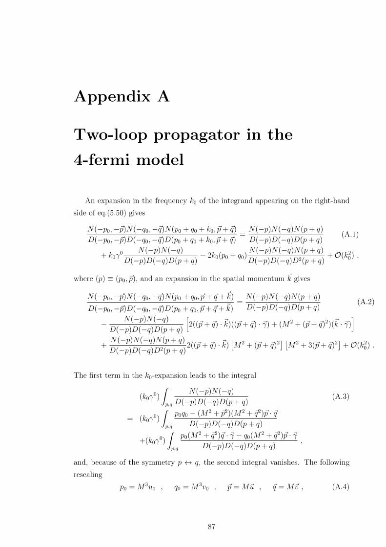
Appendix A

Two-loop propagator in the

4-fermi model

An expansion in the frequency k0 of the integrand appearing on the right-hand

side of eq.(5.50) gives

N(−p0,−~p)N(−q0,−~q)N(p0 + q0 + k0, ~p+ ~q)

D(−p0,−~p)D(−q0,−~q)D(p0 + q0 + k0, ~p+ ~q)=N(−p)N(−q)N(p+ q)

D(−p)D(−q)D(p+ q)(A.1)

+ k0γ0 N(−p)N(−q)D(−p)D(−q)D(p+ q)

− 2k0(p0 + q0)N(−p)N(−q)N(p+ q)

D(−p)D(−q)D2(p+ q)+O(k2

0) ,

where (p) ≡ (p0, ~p), and an expansion in the spatial momentum ~k gives

N(−p0,−~p)N(−q0,−~q)N(p0 + q0, ~p+ ~q + ~k)

D(−p0,−~p)D(−q0,−~q)D(p0 + q0, ~p+ ~q + ~k)=N(−p)N(−q)N(p+ q)

D(−p)D(−q)D(p+ q)(A.2)

− N(−p)N(−q)D(−p)D(−q)D(p+ q)

[2((~p+ ~q) · ~k)((~p+ ~q) · ~γ) + (M2 + (~p+ ~q)2)(~k · ~γ)

]+N(−p)N(−q)N(p+ q)

D(−p)D(−q)D2(p+ q)2((~p+ ~q) · ~k)

[M2 + (~p+ ~q)2

] [M2 + 3(~p+ ~q)2

]+O(k2

0) .

The first term in the k0-expansion leads to the integral

(k0γ0)

∫p,q

N(−p)N(−q)D(−p)D(−q)D(p+ q)

(A.3)

= (k0γ0)

∫p,q

p0q0 − (M2 + ~p2)(M2 + ~q2)~p · ~qD(−p)D(−q)D(p+ q)

+(k0γ0)

∫p,q

p0(M2 + ~q2)~q · ~γ − q0(M2 + ~q2)~p · ~γD(−p)D(−q)D(p+ q)

,

and, because of the symmetry p ↔ q, the second integral vanishes. The following

rescaling

p0 = M3u0 , q0 = M3v0 , ~p = M~u , ~q = M~v , (A.4)

87

together with a Wick rotation on u0, v0 finally leads to

(k0γ0)

∫p,q

N(−p)N(−q)D(−p)D(−q)D(p+ q)

(A.5)

= −(k0γ0)

∫d4uE(2π)4

d4vE(2π)4

u4v4 + (1 + ~u2)(1 + ~v2)~u · ~vDE(uE)DE(vE)DE(uE + vE)

, (A.6)

where DE(uE) = u24 + (1 + ~u2)2~u2.

The second term in the k0-expansion gives

−2k0

∫u,v

(p0 + q0)N(−p)N(−q)N(p+ q)

D(−p)D(−q)D2(p+ q)(A.7)

= −2(k0γ0)

∫p,q

(p0 + q0)2p0q0 − (M2 + ~p2)(M2 + ~q2)~p · ~qD(−p)D(−q)D2(p+ q)

−2k0

∫p,q

(p0 + q0)p0γ

0 ~q · ~γ (~p+ ~q) · ~γ (M2 + q2)[M2 + (~p+ ~q)2]− (p↔ q)

D(−p)D(−q)D2(p+ q),

where, by symmetry, the terms proportional to ~γ lead to a vanishing integral. After

the rescaling (A.4) and a Wick rotation, we then obtain

−2k0

∫u,v

(p0 + q0)N(−p)N(−q)N(p+ q)

D(−p)D(−q)D2(p+ q)(A.8)

= 2(k0γ0)

∫d4uE(2π)4

d4vE(2π)4

(u4 + v4)2 u4v4 + (1 + ~u2)(1 + ~v2)~u · ~vDE(uE)DE(vE)D2

E(uE + vE).

The term proportional to k0γ0 is then

(k0γ0)

∫d4uE(2π)4

d4vE(2π)4

u4v4 + (1 + ~u2)(1 + ~v2)~u · ~vDE(uE)DE(vE)DE(uE + vE)

(−1 +

2(u4 + v4)2

DE(uE + vE)

). (A.9)

For the first term in the ~k-expansion, we use the identity∫p,q

f(p, q) ~p · ~k (~p+ ~q) · ~γ =~k · ~γ

3

∫p,q

f(p, q) ~p · (~p+ ~q) , (A.10)

where f(p, q) depends on (~p)2, (~q)2 and ~p · ~q only. The rescaling (A.4) and a Wick

rotation then lead to the integral

−∫p,q

N(−p)N(−q)D(−p)D(−q)D(p+ q)

[2((~p+ ~q) · ~k)((~p+ ~q) · ~γ) + (M2 + (~p+ ~q)2)(~k · ~γ)

]= M2(~k · ~γ)

∫d4uE(2π)4

d4vE(2π)4

(1 +

5

3(~u+ ~v)2

)u4v4 + (1 + ~u2)(1 + ~v2)~u · ~vDE(uE)DE(vE)DE(uE + vE)

. (A.11)

The second term in the ~k-expansion leads to the integral

2

∫p,q

N(−p)N(−q)N(p+ q)

D(−p)D(−q)D2(p+ q)((~p+ ~q) · ~k)

[M2 + (~p+ ~q)2

] [M2 + 3(~p+ ~q)2

]= −2M2

∫u,v

u0v0 − (1 + ~u2)(1 + ~v2)~u · ~vDE(uE)DE(vE)D2

E(uE + vE)(1 + (~u+ ~v)2)(~u+ ~v) · ~γ

× (~u+ ~v) · ~k [1 + (~u+ ~v)2][1 + 3(~u+ ~v)2] , (A.12)

88

where, by symmetry, the term not proportional to ~γ vanishes. Using the identity

(A.10), a Wick rotation then leads to

2

∫p,q

N(−p)N(−q)N(p+ q)

D(−p)D(−q)D2(p+ q)((~p+ ~q) · ~k)

[M2 + (~p+ ~q)2

] [M2 + 3(~p+ ~q)2

]= −2

3M2(~k · ~γ)

∫d4uE(2π)4

d4vE(2π)4

u4v4 + (1 + ~u2)(1 + ~v2)~u · ~vDE(uE)DE(vE)D2

E(uE + vE)

× (~u+ ~v)2[1 + (~u+ ~v)2]2[1 + 3(~u+ ~v)2] . (A.13)

The term proportional to (~k · ~γ) is then

M2(~k · ~γ)

∫d4uE(2π)4

d4vE(2π)4

u4v4 + (1 + ~u2)(1 + ~v2)~u · ~vDE(uE)DE(vE)DE(uE + vE)

×(

1 +5

3(~u+ ~v)2 − 2

3(~u+ ~v)2 [1 + (~u+ ~v)2]2[1 + 3(~u+ ~v)2]

DE(uE + vE)

).(A.14)

Finally, from eqs.(A.9,A.14), the quantum corrections to the IR dispersion relation

are determined by

Ya − Za = 4g2a(3g

2a + 4g2

b )

∫d4uE(2π)4

d4vE(2π)4

Int , (A.15)

where the integrand is

Int =1

3

u4v4 + (1 + ~u2)(1 + ~v2)~u · ~vDE(uE)DE(vE)D2

E(uE + vE)(A.16)

×[(u4 + v4)2

(6 + 5(~u+ ~v)2

)− (~u+ ~v)2(1 + (~u+ ~v)2)2(2 + (~u+ ~v)2)

].

Note that in the Lorentz-symmetric case, higher orders in ~u,~v are absent and Ya =

Za. The integral (A.15) is evaluated as follows.

We can first perform the exact integration over u4, v4, using the Feynman parametri-

sation. This introduces two new variables of integration, but which lie in a compact

domain of integration:

1

DE(uE)DE(vE)D2E(uE + vE)

= 6

∫ 1

0

dx

∫ 1−x

0

dy1− x− y

[xDE(uE) + yDE(vE) + (1− x− y)DE(uE + vE)]4,

We then introduce the variables a, b, such that

u4 = s(a+ b) and v4 = t(a− b) , with s =√

1− x and t =√

1− y , (A.17)

to obtain

du4 dv4

DE(uE)DE(vE)D2E(uE + vE)

=

∫ 1

0

dx

∫ 1−x

0

dy12 da db stσ

[2st(st+ σ)a2 + 2st(st− σ)b2 +D]4,

89

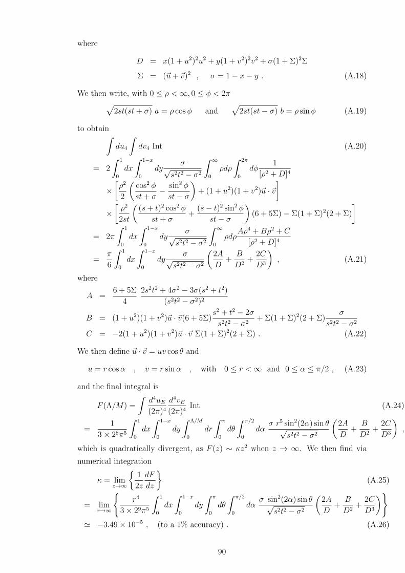
where

D = x(1 + u2)2u2 + y(1 + v2)2v2 + σ(1 + Σ)2Σ

Σ = (~u+ ~v)2 , σ = 1− x− y . (A.18)

We then write, with 0 ≤ ρ <∞, 0 ≤ φ < 2π√2st(st+ σ) a = ρ cosφ and

√2st(st− σ) b = ρ sinφ (A.19)

to obtain∫du4

∫dv4 Int (A.20)

= 2

∫ 1

0

dx

∫ 1−x

0

dyσ√

s2t2 − σ2

∫ ∞0

ρdρ

∫ 2π

0

dφ1

[ρ2 +D]4

×[ρ2

2

(cos2 φ

st+ σ− sin2 φ

st− σ

)+ (1 + u2)(1 + v2)~u · ~v

]×[ρ2

2st

((s+ t)2 cos2 φ

st+ σ+

(s− t)2 sin2 φ

st− σ

)(6 + 5Σ)− Σ(1 + Σ)2(2 + Σ)

]= 2π

∫ 1

0

dx

∫ 1−x

0

dyσ√

s2t2 − σ2

∫ ∞0

ρdρAρ4 +Bρ2 + C

[ρ2 +D]4

=π

6

∫ 1

0

dx

∫ 1−x

0

dyσ√

s2t2 − σ2

(2A

D+

B

D2+

2C

D3

), (A.21)

where

A =6 + 5Σ

4

2s2t2 + 4σ2 − 3σ(s2 + t2)

(s2t2 − σ2)2

B = (1 + u2)(1 + v2)~u · ~v(6 + 5Σ)s2 + t2 − 2σ

s2t2 − σ2+ Σ(1 + Σ)2(2 + Σ)

σ

s2t2 − σ2

C = −2(1 + u2)(1 + v2)~u · ~v Σ(1 + Σ)2(2 + Σ) . (A.22)

We then define ~u · ~v = uv cos θ and

u = r cosα , v = r sinα , with 0 ≤ r <∞ and 0 ≤ α ≤ π/2 , (A.23)

and the final integral is

F (Λ/M) =

∫d4uE(2π)4

d4vE(2π)4

Int (A.24)

=1

3× 28π5

∫ 1

0

dx

∫ 1−x

0

dy

∫ Λ/M

0

dr

∫ π

0

dθ

∫ π/2

0

dασ r5 sin2(2α) sin θ√

s2t2 − σ2

(2A

D+

B

D2+

2C

D3

),

which is quadratically divergent, as F (z) ∼ κz2 when z → ∞. We then find via

numerical integration

κ = limz→∞

1

2z

dF

dz

(A.25)

= limr→∞

r4

3× 29π5

∫ 1

0

dx

∫ 1−x

0

dy

∫ π

0

dθ

∫ π/2

0

dασ sin2(2α) sin θ√

s2t2 − σ2

(2A

D+

B

D2+

2C

D3

)' −3.49× 10−5 , (to a 1% accuracy) . (A.26)

90

Appendix B

Details of loop integrals in z = 2

QED

Throughout this chapter, we shall use dimensionless momentum 4-vectors. In

the following, kµ = (M2r0,M~r) is the external momentum, and pµ = (M2q0,M~q)

is a loop momentum to be integrated over (for scalar q0 and 3-vector q). The

graphs are calculated by first integrating over frequencies and then using the three-

dimensional spherical co-ordinates, with external space momentum ~r = (0, 0, r) and

loop momentum ~q = (q cos θ sinφ, q sin θ sinφ, q cosφ). In all but two relevant cases

(those used to calculate Z and the space part of the fermion integral) the integrands

are a function of only |q|, q0 and the angle φ between ~r and ~q. The integration

measure for q in 3− ε dimensions can therefore be written as:∫d3−εq =

∫ ∞0

q2−εdq

∫ π

0

sin1−ε φdφ

∫dΩ2−ε (B.1)

Where dΩ2−ε represents the integral over the remaining angular variables, which

evaluates to

2π

2−ε2

Γ(2−ε2

)(B.2)

In the few cases where the remaining angles cannot be eliminated, the index structure

shows that they will appear only at quadratic order, as q21 or q2

2. We can thus safely

make the substitution q21 → q2 1

2−ε sin2 φ wherever such terms appear.

In what follows, we note ∫q

≡∫d3−εqdq0

(2π)4−ε . (B.3)

B.1 Photon mass

As a check, we shall ensure the photon mass correction vanishes, as implied by

the Ward identity. For D00 and D0i we need consider only the vacuum polarisation

graph, but for Dij we must consider both photon graphs shown in the two lower

91

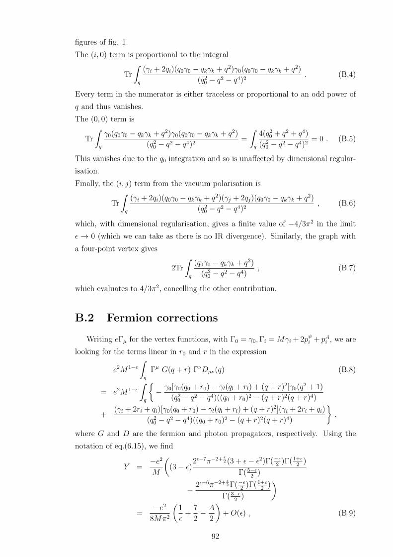
figures of fig. 1.

The (i, 0) term is proportional to the integral

Tr

∫q

(γi + 2qi)(q0γ0 − qkγk + q2)γ0(q0γ0 − qkγk + q2)

(q20 − q2 − q4)2

. (B.4)

Every term in the numerator is either traceless or proportional to an odd power of

q and thus vanishes.

The (0, 0) term is

Tr

∫q

γ0(q0γ0 − qkγk + q2)γ0(q0γ0 − qkγk + q2)

(q20 − q2 − q4)2

=

∫q

4(q20 + q2 + q4)

(q20 − q2 − q4)2

= 0 . (B.5)

This vanishes due to the q0 integration and so is unaffected by dimensional regular-

isation.

Finally, the (i, j) term from the vacuum polarisation is

Tr

∫q

(γi + 2qi)(q0γ0 − qkγk + q2)(γj + 2qj)(q0γ0 − qkγk + q2)

(q20 − q2 − q4)2

, (B.6)

which, with dimensional regularisation, gives a finite value of −4/3π2 in the limit

ε → 0 (which we can take as there is no IR divergence). Similarly, the graph with

a four-point vertex gives

2Tr

∫q

(q0γ0 − qkγk + q2)

(q20 − q2 − q4)

, (B.7)

which evaluates to 4/3π2, cancelling the other contribution.

B.2 Fermion corrections

Writing eΓµ for the vertex functions, with Γ0 = γ0,Γi = Mγi + 2pψi + pAi , we are

looking for the terms linear in r0 and r in the expression

e2M1−ε∫q

Γµ G(q + r) ΓνDµν(q) (B.8)

= e2M1−ε∫q

− γ0[γ0(q0 + r0)− γl(ql + rl) + (q + r)2]γ0(q2 + 1)

(q20 − q2 − q4)((q0 + r0)2 − (q + r)2(q + r)4)

+(γi + 2ri + qi)[γ0(q0 + r0)− γl(ql + rl) + (q + r)2](γi + 2ri + qi)

(q20 − q2 − q4)((q0 + r0)2 − (q + r)2(q + r)4)

,

where G and D are the fermion and photon propagators, respectively. Using the

notation of eq.(6.15), we find

Y =−e2

M

((3− ε)2ε−7π−2+ ε

2 (3 + ε− ε2)Γ(−ε2

)Γ(1+ε2

)

Γ(5−ε2

)

− 2ε−6π−2+ ε2 Γ(−ε

2)Γ(1+ε

2)

Γ(3−ε2

)

)=

−e2

8Mπ2

(1

ε+

7

2− A

2

)+O(ε) , (B.9)

92

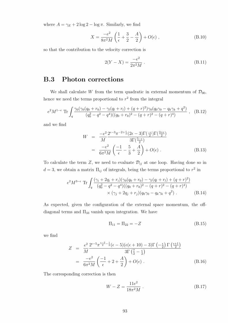
where A = γE + 2 log 2− log π. Similarly, we find

X =−e2

8π2M

(1

ε+

3

2− A

2

)+O(ε) , (B.10)

so that the contribution to the velocity correction is

2(Y −X) =−e2

2π2M. (B.11)

B.3 Photon corrections

We shall calculate W from the term quadratic in external momentum of D00,

hence we need the terms proportional to r2 from the integral

e2M1−ε Tr

∫q

γ0(γ0(q0 + r0)− γl(ql + rl) + (q + r)2)γ0(q0γ0 − qkγk + q2)

(q20 − q2 − q4)((q0 + r0)2 − (q + r)2 − (q + r)4)

, (B.12)

and we find

W =−e2

M

2ε−3π−2+ ε2 (2ε− 3)Γ(−ε

2)Γ(3+ε

2)

3Γ(5−ε2

)

=−e2

6π2M

(−1

ε− 5

3+A

2

)+O(ε) . (B.13)

To calculate the term Z, we need to evaluate Dij at one loop. Having done so in

d = 3, we obtain a matrix Πij of integrals, being the terms proportional to r2 in

e2M3−ε Tr

∫q

(γi + 2qi + ri)(γ0(q0 + r0)− γl(ql + rl) + (q + r)2)

(q20 − q2 − q4)((q0 + r0)2 − (q + r)2 − (q + r)4)

× (γj + 2qj + rj)(q0γ0 − qkγk + q2) . (B.14)

As expected, given the configuration of the external space momentum, the off-

diagonal terms and Π33 vanish upon integration. We have

Π11 = Π22 = −Z (B.15)

we find

Z =e2

M

2ε−5πε−32− 1

2 (ε− 5)(ε(ε+ 10)− 3)Γ(− ε

2

)Γ(ε+1

2

)3Γ(

72− ε

2

)=

−e2

6π2M

(−1

ε+ 2 +

A

2

)+O(ε) . (B.16)

The corresponding correction is then

W − Z =11e2

18π2M. (B.17)

93

Appendix C

Dimensional Regularisation

The method of dimensional regularisation (that is, analytically continuing the

number of spacetime dimensions, d, away from an integer value) is frequently used

as a method of regularisation in gauge theories, as it allows one to preserve the

Ward identity (or its equivalents) in the regularised theory, unlike a high-momentum

cuttoff which may violate that symmetry. “Divergences” are then represented as

poles in the parameter ε = d − d0 , where d0 is the usual number of dimensions (4

in most cases).

As we work with Lorentz-violating theories in which there is a distinguished

time co-ordinate, we shall in practice analytically continue the number of space

dimensions only.

C.1 Finiteness of naıvely divergent integrals

There is a feature of dimensional regularisation, not often seen in the integrals

derived from four dimensional QFT, but fairly common in odd dimensions (and

the anisotropic models with which we work in this thesis); that is, an integral that

appears UV divergent in d0 dimensions may have an expression in d 6= d0 that can

be analytically continued back to d0 without encountering any poles.

This is shown explicitly in chapter 6 where an integral, for ε 6= 0, can be written

as a product of Gamma functions that can be analytically continued in the usual

fashion back to ε = 0 to give a finite answer. It can also be seen in the following toy

example: consider the following integral of a form one often sees in QFT calculations

(where n is usually the number of dimensions, plus a constant)

I(n) =

∫ ∞0

dxxn

(k2 +m2)3(C.1)

If one were to impose a UV cutoff, one would see that this integral diverges as Λn−5

and so one would certainly expect it to be divergent at, say, n = 6. However, away

94

from integer values of n, this integral can be evaluated exactly as

I(n) =mn−5

(5− n)

Γ(n+12

)Γ(7−n2

)

Γ(3)(C.2)

This expression can then be continued analytically to the whole plane, less a few

isolated singularities; in particular, it is regular at n = 6 (and any other even value

of n). Such behaviour is generic in analytic continuation, indeed, it is a general

property of limits and one should not be overly surprised.

In general, dimensional regularisation can “see” only logarithmic divergences

(that is, those that would go as log Λ if we had introduced a cutoff), whereas those

with purely polynomial divergences give finite contributions as ε → 0. This can

be seen schematically as follows: consider a polynomially divergent integral in d

dimensions, I(d), we shall isolate its divergent part as

I(d) = (finite) + C

∫ddkkn , (C.3)

where C is some constant coefficient. Simple dimensional analysis gives [∫ddkkn] =

n+ d and the second term above would indeed diverge as Λn+d, were there a cutoff.

However, the integral above has no mass scales and so, if it is to have any finite

value at all, it must vanish. Such a result is of course, easily analytically continued

to almost all values of d. So for consistency, under dimensional regularisation, we

must take ∫ddkkn = 0, (d+ n 6= 0) . (C.4)

The only exception to the above is at d + n = 0, where the integral is dimension-

less and the divergence is logarithmic. One could consider this the m → 0 limit of

equation C.2.

This behaviour is not a problem for renormalisation group studies with dimen-

sional regularisation, as it is the logarithmically divergent terms that determine the

beta functions. The higher-order divergences are of course still “encoded” in the

regularised expression, as poles at other integer values of ε.

C.2 Divergence cancelling

We emphasise that the cases considered above are technically distinct from the

finite results obtained for integrals such as∫ddx

4xµxν − x2ηµν(x2 −m2)3

(C.5)

95

at d = 4, as are discussed in [76]. By power counting this integral is logarithmically

divergent and indeed is not well-defined at d = 4. If one splits the integrand into

several parts, or divides the domain of integration into several angular regions, one

finds terms in each that require regularisation and give logarithmic divergences.

However, upon summing these terms, the divergences cancel exactly, leaving a finite

result as d→ 4.

96

Bibliography

[1] J. Alexandre, J. Brister and N. Houston, Phys. Rev. D 86 (2012) 025030

[arXiv:1204.2246 [hep-ph]].

[2] J. Alexandre and J. Brister, Phys. Rev. D 88 (2013) 6, 065020 [arXiv:1307.7613

[hep-th]]; J. Alexandre and A. Vergou, Phys. Rev. D 83 (2011) 125008

[arXiv:1103.2701 [hep-th]].

[3] J. Alexandre and J. Brister, Phys. Rev. D 92 (2015) 2, 024025

[arXiv:1505.01392 [hep-th]].

[4] P. Horava, Phys. Rev. D 79 (2009) 084008 [arXiv:0901.3775 [hep-th]].

[5] R. Iengo, J. G. Russo, M. Serone, JHEP 0911 (2009) 020. [arXiv:0906.3477

[hep-th]].

[6] O. W. Greenberg, Phys. Rev. Lett. 89 (2002) 231602 [hep-ph/0201258].

[7] V. A. Kostelecky and N. Russell, Rev. Mod. Phys. 83 (2011) 11

[arXiv:0801.0287 [hep-ph]].

[8] D. Colladay and V. A. Kostelecky, Phys. Rev. D 58 (1998) 116002 [hep-

ph/9809521].

[9] A. Kobakhidze and B. H. J. McKellar, Phys. Rev. D 76 (2007) 093004

[arXiv:0707.0343 [hep-ph]].

[10] S. Hossenfelder, arXiv:1504.06070 [gr-qc].

[11] J. H. Cooperman, arXiv:1410.0670 [gr-qc].

[12] J. Ambjorn, A. Goerlich, J. Jurkiewicz and R. Loll, arXiv:1305.6680 [gr-qc].

[13] G. Amelino-Camelia, Symmetry 2 (2010) 230 [arXiv:1003.3942 [gr-qc]].

[14] J. Magueijo and L. Smolin, Class. Quant. Grav. 21 (2004) 1725 [gr-

qc/0305055].

[15] R. Garattini and E. N. Saridakis, arXiv:1411.7257 [gr-qc].

97

[16] E.M. Lifshitz, Zh. Eksp. Toer. Fiz. 11, 255; 269 (1941).

[17] J. Alexandre, K. Farakos and A. Tsapalis, Phys. Rev. D 81 (2010) 105029

[arXiv:1004.4201 [hep-th]].

[18] 3] M. V. Ostrogradsky, Mem. Acad. St. Petersbourg VI 4, 385 (1850)

[19] D. Anselmi and M. Halat, Phys. Rev. D 76 (2007) 125011 [arXiv:0707.2480

[hep-th]].

[20] J. Alexandre, arXiv:1009.5834 [hep-ph].

[21] T. Jacobson, Phys. Rev. D 81 (2010) 101502 [Phys. Rev. D 82 (2010) 129901]

[arXiv:1001.4823 [hep-th]].

[22] T. Jacobson, Phys. Rev. D 89 (2014) 8, 081501 [arXiv:1310.5115 [gr-qc]].

[23] N. Arkani-Hamed, P. Creminelli, S. Mukohyama and M. Zaldarriaga, JCAP

0404 (2004) 001 [hep-th/0312100].

[24] P. Horava and C. M. Melby-Thompson, Gen. Rel. Grav. 43 (2011) 1391

[arXiv:0909.3841 [hep-th]].

[25] J. Alexandre, Int. J. Mod. Phys. A 26 (2011) 4523 [arXiv:1109.5629 [hep-ph]].

[26] D. Anselmi, Eur. Phys. J. C65 (2010) 523-536. [arXiv:0904.1849 [hep-

ph]]; A. Dhar, G. Mandal, S. R. Wadia, Phys. Rev. D80 (2009) 105018.

[arXiv:0905.2928 [hep-th]].

[27] D. Anselmi and M. Taiuti, Phys. Rev. D 81 (2010) 085042 [arXiv:0912.0113

[hep-ph]].

[28] F. Benatti and R. Floreanini, Phys. Rev. D 64 (2001) 085015 [hep-

ph/0105303].

[29] V. A. Kostelecky and M. Mewes, Phys. Rev. D 70 (2004) 031902 [hep-

ph/0308300]; V. A. Kostelecky and M. Mewes, Phys. Rev. D 69 (2004) 016005

[hep-ph/0309025]; V. Barger, D. Marfatia and K. Whisnant, Phys. Lett. B 653

(2007) 267 [arXiv:0706.1085 [hep-ph]].

[30] V. Barger, J. Liao, D. Marfatia and K. Whisnant, Phys. Rev. D 84 (2011)

056014 [arXiv:1106.6023 [hep-ph]].

[31] J. Magueijo, arXiv:1109.6055 [hep-ph].

[32] T. R. Morris, arXiv:1110.2463 [hep-ph]; H. Minakata and A. Y. .Smirnov,

arXiv:1202.0953 [hep-ph].

98

[33] M. K. Volkov and A. E. Radzhabov, hep-ph/0508263.

[34] V. P. Gusynin, V. A. Miransky and I. A. Shovkovy, Nucl. Phys. B 462

(1996) 249 [arXiv:hep-ph/9509320]; Phys. Rev. Lett. 73 (1994) 3499 [Erratum-

ibid. 76 (1996) 1005] [arXiv:hep-ph/9405262]; Phys. Rev. D 52 (1995) 4747

[arXiv:hep-ph/9501304]; J. Alexandre, K. Farakos and G. Koutsoumbas,

Phys. Rev. D 64 (2001) 067702; Phys. Rev. D 63 (2001) 065015 [arXiv:hep-

th/0010211]; J. Alexandre, K. Farakos, S. J. Hands, G. Koutsoumbas and

S. E. Morrison, Phys. Rev. D 64 (2001) 034502 [arXiv:hep-lat/0101011];

J. Alexandre, Phys. Rev. D 63 (2001) 073010 [hep-th/0009204].

[35] J. Alexandre, J. Leite and N. E. Mavromatos, Phys. Rev. D 90 (2014) 4,

045026 [arXiv:1404.7429 [hep-th]].

[36] J. Alexandre and A. Vergou, Phys. Rev. D 83 (2011) 125008 [arXiv:1103.2701

[hep-th]]; J. Alexandre and N. E. Mavromatos, Phys. Rev. D 83 (2011) 127703

[arXiv:1104.1583 [hep-th]]; J. Alexandre and N. E. Mavromatos, Phys. Rev.

D 84 (2011) 105013 [arXiv:1108.3983 [hep-ph]].

[37] F. Cooper, B. Mihaila and J. F. Dawson, Phys. Rev. D 70 (2004) 105008

doi:10.1103/PhysRevD.70.105008 [hep-ph/0407119].

[38] T. Schwetz, M. A. Tortola and J. W. F. Valle, New J. Phys. 10 (2008) 113011

[arXiv:0808.2016 [hep-ph]].

[39] W. Wetzel, Phys. Lett. B 153 (1985) 297; C. Luperini and P. Rossi, Annals

Phys. 212 (1991) 371; N. D. Tracas and N. D. Vlachos, Phys. Rev. D 43

(1991) 3447.

[40] P. R. S. Gomes and M. Gomes, arXiv:1107.6040 [hep-th].

[41] M. J. Longo, Phys. Rev. D 36 (1987) 3276.

[42] J. Alexandre, K. Farakos, P. Pasipoularides and A. Tsapalis, Phys. Rev. D 81

(2010) 045002 [arXiv:0909.3719 [hep-th]].

[43] D. Anselmi, Annals Phys. 324 (2009) 874 [arXiv:0808.3470 [hep-th]]; Annals

Phys. 324 (2009) 1058 [arXiv:0808.3474 [hep-th]].

[44] C. F. Farias, M. Gomes, J. R. Nascimento, A. Y. .Petrov and A. J. da Silva,

Phys. Rev. D 85 (2012) 127701 [arXiv:1112.2081 [hep-th]].

[45] J. Alexandre, arXiv:1009.5834 [hep-ph]. J. Alexandre and A. Vergou, Phys.

Rev. D 83 (2011) 125008 [arXiv:1103.2701 [hep-th]].

99

[46] A. Padilla, J. Phys. Conf. Ser. 259 (2010) 012033 [arXiv:1009.4074 [hep-th]].

[47] T. P. Sotiriou, J. Phys. Conf. Ser. 283 (2011) 012034 [arXiv:1010.3218 [hep-

th]].

[48] M. Visser, J. Phys. Conf. Ser. 314 (2011) 012002 [arXiv:1103.5587 [hep-th]].

[49] T. P. Sotiriou, M. Visser and S. Weinfurtner, JHEP 0910 (2009) 033-065

[arXiv:0905.2798 [hep-th]]; C. Charmousis, G. Niz, A. Padilla and P. M. Saffin,

JHEP 0908 (2009) 070-086 [arXiv:0905.2579 [hep-th]].

[50] D. Blas, O. Pujolas and S. Sibiryakov, Phys. Lett. B 688 (2010) 350

[arXiv:0912.0550 [hep-th]].

[51] M. Henneaux, C. Teitelboim and J. Zanelli, Nucl. Phys. B 332 (1990) 169.

[52] I. Kimpton and A. Padilla, JHEP 1007 (2010) 014 [arXiv:1003.5666 [hep-th]].

[53] J. Bellorin, A. Restuccia and A. Sotomayor, Phys. Rev. D 87 (2013) 8, 084020

[arXiv:1302.1357 [hep-th]].

[54] A. Contillo, S. Rechenberger and F. Saueressig, JHEP 1312 (2013) 017

[arXiv:1309.7273 [hep-th]]; G. D’Odorico, F. Saueressig and M. Schutten,

Phys. Rev. Lett. 113 (2014) 17, 171101 [arXiv:1406.4366 [gr-qc]].

[55] M. Reuter and F. Saueressig, arXiv:0708.1317 [hep-th]; D. Benedetti,

P. F. Machado and F. Saueressig, Mod. Phys. Lett. A 24 (2009) 2233

[arXiv:0901.2984 [hep-th]]; J. A. Dietz and T. R. Morris, JHEP 1301 (2013)

108 [arXiv:1211.0955 [hep-th]]; K. Falls, D. F. Litim, K. Nikolakopoulos and

C. Rahmede, arXiv:1301.4191 [hep-th].

[56] C. Anderson, S. J. Carlip, J. H. Cooperman, P. Horava, R. K. Kommu and

P. R. Zulkowski, Phys. Rev. D 85 (2012) 044027 [arXiv:1111.6634 [hep-th]].

[57] B. F. Li, A. Wang, Y. Wu and Z. C. Wu, arXiv:1408.2345 [hep-th].

[58] A. M. da Silva, Class. Quant. Grav. 28 (2011) 055011 [arXiv:1009.4885 [hep-

th]];

[59] C. Germani, A. Kehagias and K. Sfetsos, JHEP 0909 (2009) 060

[arXiv:0906.1201 [hep-th]].

[60] I. Kimpton and A. Padilla, JHEP 1304 (2013) 133 [arXiv:1301.6950 [hep-th]].

[61] N. Frusciante, M. Raveri, D. Vernieri, B. Hu and A. Silvestri, arXiv:1508.01787

[astro-ph.CO].

100

[62] P. Horava and C. M. Melby-Thompson, Phys. Rev. D 82 (2010) 064027

[arXiv:1007.2410 [hep-th]].

[63] E. Abdalla and A. M. da Silva, Phys. Lett. B 707 (2012) 311-314

[arXiv:1111.2224 [hep-th]].

[64] K. Lin, S. Mukohyama and A. Wang, Phys. Rev. D 86 (2012) 104024

doi:10.1103/PhysRevD.86.104024 [arXiv:1206.1338 [hep-th]].

[65] K. Lin and A. Wang, Phys. Rev. D 87 (2013) 8, 084041

doi:10.1103/PhysRevD.87.084041 [arXiv:1212.6794 [hep-th]].

[66] J. Alexandre and P. Pasipoularides, Phys. Rev. D 83 (2011) 084030

[arXiv:1010.3634 [hep-th]]; J. Greenwald, V. H. Satheeshkumar and A. Wang,

JCAP 1012 (2010) 007 [arXiv:1010.3794 [hep-th]];

[67] J. Alexandre and M. Kostacinska, Galaxies 2 (2014) 1 [arXiv:1303.1394 [hep-

th]].

[68] A. Wang and Y. Wu, Phys. Rev. D 83 (2011) 044031 [arXiv:1009.2089 [hep-

th]]; T. Zhu, F. -W. Shu, Q. Wu and A. Wang, Phys. Rev. D 85 (2012) 044053

[arXiv:1110.5106 [hep-th]]; Y. Huang, A. Wang and Q. Wu, JCAP 1210 (2012)

010 [arXiv:1201.4630 [gr-qc]]; T. Zhu, Y. Huang and A. Wang, JHEP 1301

(2013) 138 [arXiv:1208.2491 [hep-th]]; Y. Huang and A. Wang, Phys. Rev. D

86 (2012) 103523 [arXiv:1209.1624 [hep-th]]; Y. Huang, A. Wang, R. Yousefi

and T. Zhu, Phys. Rev. D 88 (2013) 2, 023523 [arXiv:1304.1556 [hep-th]].

[69] J. Kluson, Phys. Rev. D 83 (2011) 044049 [arXiv:1011.1857 [hep-th]]; K. Lin,

S. Mukohyama and A. Wang, Phys. Rev. D 86 (2012) 104024 [arXiv:1206.1338

[hep-th]].

[70] R. H. Sanders, Phys. Rev. D 84 (2011) 084024 [arXiv:1105.3910 [gr-qc]].

[71] L. Blanchet and S. Marsat, arXiv:1205.0400 [gr-qc].

[72] M. Pospelov and Y. Shang, Phys. Rev. D 85 (2012) 105001 [arXiv:1010.5249

[hep-th]].

[73] P. O. Mazur and E. Mottola, Nucl. Phys. B 341 (1990) 187. doi:10.1016/0550-

3213(90)90268-I

[74] J. Alexandre and J. Leite, arXiv:1506.03755 [hep-ph].

[75] G. Leibbrandt, Rev. Mod. Phys. 47 (1975) 849.

[76] S. Weinzierl, arXiv:1402.4407 [hep-ph].

101

[77] J. Alexandre and J. Leite, arXiv:1506.03755 [hep-ph].

[78] G. Degrassi, S. Di Vita, J. Elias-Miro, J. R. Espinosa, G. F. Giudice, G. Isidori

and A. Strumia, JHEP 1208, 098 (2012) [arXiv:1205.6497 [hep-ph]].

[79] M. Herranen, T. Markkanen, S. Nurmi and A. Rajantie, Phys. Rev. Lett. 113

(2014) 21, 211102 [arXiv:1407.3141 [hep-ph]].

[80] J. Abraham et al. [Pierre Auger Collaboration], Phys. Lett. B 685 (2010) 239

[arXiv:1002.1975 [astro-ph.HE]].

[81] G. Rubtsov, P. Satunin and S. Sibiryakov, Phys. Rev. D 89 (2014) 12, 123011

[arXiv:1312.4368 [astro-ph.HE]].

[82] W. Xue, arXiv:1008.5102 [hep-th]; M. Gomes, J. Queiruga and A. J. da Silva,

arXiv:1506.01331 [hep-th].

102