77 - nasa · uniformly cold wall boundary condition by roger bell stewart thesis submitted to the...
TRANSCRIPT
NASA-TN-X-69220) NUMERICAL ANDEXPERIMENTAL STUDIES OF THE NATURALCONVECTION FLOW WITHIN A HORIZONTALCYLINDER SUBJECTED TO A UNIFORMLY COLDWALL (NASA) 140 p HC $9.00 CSCL 20D
UnclasG3/12 68629
NUMERICAL AND EXPERIMENTAL STUDIES OF THE
NATURAL CONVECTION FLOW WITHIN A HORIZONTAL CYLINDER SUBJECTED TO A
UNIFORMLY COLD WALL BOUNDARY CONDITION
By
Roger Bell Stewart
Thesis submitted to the Graduate Faculty of the
Virginia Polytechnic Institute and State University
in partial fulfillment of the requirements for the degree of
DOCTOR OF PHILOSOPHY
in
Aerospace Engineering
October 1972
77
https://ntrs.nasa.gov/search.jsp?R=19730012551 2018-09-03T15:08:26+00:00Z
NUMERICAL AND EXPERIMENTAL STUDIES OF THE
NATURAL CONVECTION FLOW WITHIN A HORIZONTAL CYLINDER SUBJECTED TO A
UNIFORMLY COLD WALL BOUNDARY CONDITION
by
Roger Bell Stewart
Thesis submitted to the Graduate Faculty of the
Virginia Polytechnic Institute and State University
in partial fulfillment of the requirements for the degree of
DOCTOR OF PHILOSOPHY
in
Aerospace Engineering
APPROVED:
Dr. J. A. Schetz, Chairman
Dr. W. B. Olstad
. J. E. Kaiser, Jr.
Dr. C. H. Lewis
--Dr. Yau uDr! Yau Wu
October 1972
Blacksburg, Virginia
LIZ
(ABSTRACT)
Numerical solutions are obtained for the quasi-compressible Navier-
Stokes equations governing the time dependent natural convection flow
within a horizontal cylinder. The early time flow development and wall
heat transfer is obtained after imposing a uniformly cold wall boundary
condition on the cylinder. Solutions are also obtained for the case of
a time varying cold wall boundary condition. Windward explicit differ-
encing is used for the numerical solutions. The viscous truncation
error associated with this scheme is controlled so that first order
accuracy is maintained in time and space. The results encompass a
range of Grashof numbers from 8.34 x 10⁴ to 7 x 10⁷ which is within the
laminar flow regime for gravitationally driven fluid flows. Experiments
within a small scale instrumented horizontal cylinder revealed the time
development of the temperature distribution across the boundary layer
and also the decay of wall heat transfer with time. Agreement between
measured temperature distributions and the numerical solutions was
generally good. The time decay of the dimensionless ratio Nu/G1/4is
r
found numerically and experimentally and, over most of the cylinder wall,
good agreement is obtained between these two results. The numerical
results indicate that the fluid exhibits a strong tendency to resist
first order motion within the inner core region. The early establish-
ment of a shallow positive upward temperature gradient within the core
enhances its stability. No first order vortical motion is induced by
the boundary layer and this is attributed in part to the fluid decelera-
tion near the bottom of the cylinder along with expulsion of fluid from
-7 ?
the boundary layer in the lower portions of the cylinder.
i/-E
ACKNOWLEDGMENTS
The author wishes to express his appreciation to Dr. J. A. Schetz
for his helpful suggestions and criticisms throughout this effort, and
to the entire graduate committee for their review and suggestions on
this thesis.
The author is also indebted to the National Aeronautics and Space
Administration for permitting material obtained from research conducted
at the Langley Research Center to be used in this thesis.
Particular thanks are due Miss Lillian R. Boney for programming
the numerical work and the computer plotting routines. The author would
also like to thank Mr. George W. Johnson for setting up all of the
experimental apparatus as well as carrying out all of the automatic data
gathering operations. Thanks are due Mrs. Gloria Evans for typing the
rough draft and Joanne Halvorson who typed the final draft.
Finally the author is greatly indebted to his wife and three sons
for their patient and encouraging help throughout the entire graduate
effort.
i
TABLE OF CONTENTSPage
Acknowledgements . . . . . . . . . . . . . . . . i
Table of Contents. . . . . . . . . . . . . . . . . . . .... ii
List of Figures. . . . . . . . . . . . . . . . . ... . .-.. ii
List of Symbols. . . . . . . . . . . . . . . . . . . . .. vi
CHAPTER
I. Introduction. . . . . . . . . . . . . . . . . . ... 1
II. Physical Description of the Problem .. . . . . . . . 5
III. Mathematical Formulation of the Governing Equations . . . 7
IV. Development of the Finite Difference Approximation tothe Governing Equations ................. 16
V. Numerical Solutions ................... 22
A. Constant Wall Temperature Boundary Condition . . . 22
B. Time Varying Wall Temperature Boundary Condition . 29
VI. Experimental Apparatus. . . . . . . . . . . . . . . .. 35
VII. Discussion of Experimental Results. ......... . 41
VIII. Conclusions . . . . . . . . . . . . . . . . . . .... 47
IX. Bibliography. . . . . . . . . . . . . . . . . . ... 50
X. Appendix A - Stability Analysis . .-. . . . . . . . . 52
XI. Appendix B - Thermocouple Errors ............ 60
Table I ................... ......... 67
Figures. ................... ........ 68-128
VITA ................... .... 129
ii
LIST OF FIGURES
Figure
1. Schematic diagram of horizontal Cylinder with coordinatesystem and wall boundary conditions . . . . . . . . . . . . . .
2. Finite difference grid network . . . . . . . . . . . . . . . .
3. Flow diagram for numerical calculations . . . . . . . . . . . .
a. Continued ......................b. Continued . . . . . . . . . . . . . . . . . . . . . .c. Continued . . . . . . . . . . . . . . . . . . . . . .d. Concluded ......................
4. Azimuthal velocity distribution for a Grashof number of7xo107 . . . . . . . . . . . . . . . . . . . . . . . . .
a. 0 = 90 ..........................b. e = 23.70 .c. 0 = 1610.........................
5. Radial velocity distribution within the Cylindera. e = 900 ..........................b. 0 = 23.70 ......... .c. = 1610d. R = .44.
6. Temperature distribution within the Cylinder
a. 8 = 900 ....................b. e = 23.70 ......... .c. 0 = 1610...................
7. Dimensionless wall heat transfer decay with time . . . . . . .
8. Temperature distribution within the core showing a positiveupward gradient ........................
9. The Nusselt-Grashof relation for a time dependent naturalconvection flow ........................
10. The effects of radial grid refinedment
a. Temperature distribution . . . . . . . . . . . .b. Azimuthal velocity . . . . . . . . . . . . . . . . . . .
iii
Page
68
69
70
70717273
747576
77787980
818283
84
85
86
8788
. .
. .
.
.
. . . . .
.$. . .
.$. . .
11. Velocity and temperature distributions for a Grashofnumber of 8.34 x 10 . . . . . . . . . . . . . . . . . . . 89
a. Azimuthal velocity . . . .. . 89b. Radial velocity . . . . . . . . . . . . . . . . . . . 90c. Temperature .................... .. 91d. Nusselt-Grashof Relation . . . . . . . . . . ... 92
12. Azimutha velocity distribution for a Grashof number of1.2 x 10 ....................... 93
13. Time dependent wall temperature decay from the onedimensional heat conduction solution . . . . . . . . . . . 94
14. Azimuthal velocity distrubution for a time dependent walltemperature boundary condition . . . . . . . . . . .... 95
15. Time dependence of the Grashof number for a time dependentwall temperature boundary condition . . . . . . . . . . . 96
16a. Temperature distribution for a time dependent wall tempera-ture boundary condition .97
16b. Temperature distributions for constant and variable walltemperature boundary conditions . . . . . . . . . . . . . 98
17. Comparison of azimuthal velocity distribution for constantand variable wall temperature boundary conditions ... 99a. Dimensionless time T = 8.5 . . . . . . . . . . ... 99b. Dimensionless time T = 26.2 . . . . . . . . . . .. 100
18. Nusselt-Grashof relation for a time dependent wall boundarycondition . . . . . . . . . . . . . . . .... .. . . . 101
19. Oscilloscope photographs of fluid element displacementsfrom the numerical solutions for natural convection flowwithin a horizontal cylinder . . . . . . . . . . . .. 102
a. t = O0; t = 1.97 sec. . . . . . . . . . . . . . 102b. t = 3.04; t = 3.86 . . 103c. t = 4.54; t = 5.13 .104d. t = 5.67; t = 6.15 . . . . . . . . . . . . . . . 105e. t = 6.60 . . . . . . . . . . . . . . . 106
20a. Photograph of natural convection chamber . . . . . . . . . 107
20b. Schematic of natural convection apparatus . . . . . . . . 108
21. Cooling manifold for natural convection chamber .... 109
iv
22. Boundary layer thermocouple installation. . . . . . . . . . 110
23. Vertical flat plate apparatus for natural convection velocitymeasurements. . . . . . . . . . . . . . . . . . . . . . . . 111
a. Side view ................... l..... 111b. Front view . . . . . . . . . . . ....... . . . . . 112
24. Experimental temperature distributions for a time dependentwall boundary condition with NG ax= 7 x 10⁷.. . 113r max
a. at t = 1.2 seconds . . . . . . . . . . . . . . . .113b. at t = 4.0 seconds . . . . . . . . . . . . . . . . . 114c. at t = 8.0 seconds ................... 115
25. Experimental boundary layer decay at different azimuthallocations ........................... 116
a. = Tr/2; R=.966 .................... 116b. e = 700, R = .966 ..................... 117c. e = 0 , R = .966 ................... l. 118
26. Measured pressure decay within the horizontal cylinder. . . 119
27. The Nusselt-Grashof relation for a time dependent wallboundary condition. ................... .. 120
28. Experimental radial temperature distribution ........ 121
a. e = f1/2; t = 4.0 seconds. ................ 121b. 0 = ¶r/2; t = 8.0 seconds. ................ 122
29. Experimental radial temperature distributions forNG = 7x10 7 .................. .... 123r max
a. e = 700; t = 4.0 seconds . . . . . .. . .123b. 0 = 70 ; t = 8.0 seconds ................. 1 24
30. Experimental radial temperature distribution forNG = 1.8 x 10. ..................... 125r max
a. e = 7r/2; t = 2.0 seconds . . . . . . . . .125b. 0 = a/2; t = 4.0 seconds . . . . . . . .. 126
31. Experimental boundary layer temperature decay at 0 = x/2;R = .966 and NG = 1.3 x 10 . ... ... ....... 127r max
32. The Nusselt Grashof relation for a time dependent wallboundary condition and a maximum Grashof number of6.5 x 105 ................... 128
v
LIST OF SYMBOLS
a dimensionless constant defined in equation 5.8 and also in
appendix A.
b dimensionless constant defined in equation 5.8 and also in
appendix A.
c dimensionless constant
C specific heat at constant pressureP
d diameter of cylinder
g gravitational constant
G Grashof Number = r V2 T
h heat transfer coefficient
k thermal conductivitycvi
N Prandtl number = Ppr k
N Nusselt number defined by equation 5.1u
p pressure
P dimensionless pressure
P* dimensionless dynamic pressure
r radial distance from center of cylinder
R dimensionless radial distance from center of cylinder
AR distance between two successive radial grid points
Rea computational cell Reynolds number = UARvG
t time
T temperature
T temperature of slab surface given by equation 5.6xo
vi
u azimuthal velocity
U dimensionless azimuthal velocity
v radial velocity
V dimensionless radial velocity
x distance into cylinder wall
a artificial viscosity defined by equation 4.1e
a temperature difference given by equation 3.9
volumetric coefficient of expansion for a perfect gas
p fluid density
dimensionless fluid density
dimensionless temperature function defined by equation 3.9
dimensionless temperature function defined by equation 5.6
e azimuthal coordinate
Ae distance between two successive azimuthal grid points
T dimensionless time
AT dimensionless time increment
dynamic viscosity
V kinematic viscosity
hi Characteristic value (eigenvalue) for amplification matrix
in energy stability analysis. See equation A-8
h2 Characteristic value (eigenvalue) for amplification matrix
in momentum stability analysis. See equation A-9
Subscripts
i initial value at time = o
vii
j azimuthal grid point location
1 radial grid point location
w value at cylinder wall
Superscripts
n present value of time also summation index in equation 5.6
n + 1 new value of time
viii
INTRODUCTION
Chapter I
Natural convection flows within closed containers have intrigued
mathematicians and fluid dynamicists for many years. Part of the
motivation for understanding such flows was based upon an early
realization that many practical engineering situations are governed by
gravitationally driven fluid flows. Present day interest is concerned
with the flow of fluids within pipes, nuclear reactor cooling systems,
turbine blades, and stationary containers. These fluid flows may be
significantly influenced by natural or induced body forces. The
resultant fluid motion and heat transfer are the principle features of
interest and it is toward an understanding of these features that most
studies have been directed. The early work by Nusselt (reference 1),
Hermann (reference 2), Beckmann (reference 3), and Hermann (reference
4) established both the appropriate governing equations as well as the
general relationship between the non-dimensional heat transfer and the
Grashof number for external flows over cylindrical configurations.
Numerous experimental studies have confirmed the theoretical findings
(reference 5 through 7) for large values of the Grashof number wherein
a boundary-layer flow is present. Not until the work reported by
Ostrach (reference 8), Lewis (reference 9), Batchelor (reference 10),
and Pillow (reference 11) was the internal natural convection problem
given a general theoretical treatment comparable to the external
problem. More recent analytical studies involving somewhat restricted
1
2
wall boundary conditions have been reported by De Vahl Davis
(reference 12), Weinbaum (reference 13), Menold (reference 14), Hantman
and Ostrach, (reference 15) and Gill (reference 16).
The principal problem that has thus far prevented a general
analytical solution stems from the coupling between the boundary
layer flow near the walls of the container and the core flow that is
driven by the boundary layer flow. In formulating the problem in terms
of a stream function most of the previous investigators except Hantman
and Ostrach (reference 15) have been faced with the necessity of
specifying a core stream function behavior that is not known a priori.
Thus, depending upon specified wall boundary conditions, the core
has been assumed to have either an isothermal constant vorticity
character or to be stratified with streamlines extending into the
boundary layer. Both analytical solutions and experiments have shown
that two entirely different flow configurations are possible. If the
flow is heated from below, the core streamlines are closed and the core
is isothermal. If the wall boundary condition is such that heating
occurs from the side, the core is stratified with isotherms and
streamlines coinciding. The studies reported thus far are not able to
predict the critical heating phase angle at which a rotating flow
configuration changes to a stratified flow configuration. The Oseen
linearization used by Weinbaum does not help the problem because this
approximation decouples the core flow from the boundary layer flow.
The core is expected to be closely coupled to the boundary layer flow
because it is driven by the boundary layer.
3
A related problem with less troublesome boundary conditions is
that of a horizontal cylinder with one half of its bounding walls
raised to a constant, uniform temperature and the other half lowered
an equal amount below the initial fluid temperature. Thus a rotating
boundary-layer flow encircles the inside cylindrical walls with the
flow rising over one half the circumference and falling over the other
half. This problem was studied numerically by Hellums (reference 16).
Hellums used what is now termed the windward or donor cell differencing
technique for the time dependent problem starting from initially imposed
wall boundary conditions. He obtained numerical solutions for the
velocity, temperature, and heat transfer distributions within the
cylinder. Because fluid is both entrained and ejected by the boundary-
layer flow, the windward finite differencing scheme is quite suitable
for this type of problem. Hellums was able to make favorable compari-
sons between his solutions and experiments carried out by Martini and
Churchill (reference 17). These comparisons were possible for the
steady state flow only. No unsteady flow measurements were reported.
For steady state flow, Hellums verified the relationship between the
Nusselt number and Grashof number; Nu = C G1 / 4 both from a formalr
derivation of the dimensionless governing equations and from the
resultant numerical solutions. For unsteady flow the coefficient C
can be expected to be time dependent. The work reported by Hellums
is closely related to the present study and will be discussed in more
detail in the chapters following. At the present time only a very few
of the possible boundary conditions that could be imposed on a
4
horizontal cylinder have been studied and with only partial success
in most of the cases reported.
The work reported here represents an attempt to clarify the flow
resulting from a new wall boundary condition that has not been
here-to-fore studied for the internal flow problem. A uniform cold
wall is established at time zero and the early time development of the
fluid motion is studied. The fluid is initially at rest and will also
return to rest at very large times after flow initiation. Thus a
steady state is not of interest in the present work. In addition,
solutions are obtained for the case in which the wall temperature
decays with time. This problem corresponds to experimental boundary
conditions that were imposed within a small cylinder in the present
work. The experiments are described and a discussion of the relation-
ship between the numerical work and the experimental work is given.
A Physical Description of the Problem
Chapter II
The geometry and nomenclature of the horizontal cylinder to be
studied is shown in figure 1. The cylinder is of semi infinite length
to allow a region of two dimensional flow to existl. One practical
application for such a geometry is related to a large blowdown wind
tunnel storage facility in which the major heat loss to the walls
occurs due to gravitationally driven natural convection flows. When a
hot gas is stored in such a tank appreciable azimuthal gas flow occurs
due to the imbalance between the gravitational body forces and the
existing hydrostatic pressure gradient in the fluid. The gas, which is
air, is initially at rest with a balance between the body force and the
hydrostatic pressure gradient. The gas is initially at a uniform
temperature T.. At time zero, a uniform cold wall is imposed on the
cylinder, and the resulting conduction of heat out of the gas near the
wall causes the convective motion to begin. As the flow develops, a
thin boundary layer is formed near the wall and this layer thickens
with time. The initially motionless inner fluid (the core) is driven
by the boundary layer flow and gives up energy to the heat conducting
boundary layer fluid. As time progresses the boundary layer will
affect the inner-most regions of the core flow and eventually the gas
can be expected to give up all of its excess energy to the cold wall.
1A two dimensional flow within a horizontal cylinder has been observedby Brooks and Ostrach (reference 21).
5
6
When this happens the fluid will be once again at rest with a uniform
temperature now equal to the wall temperature. Several distinct fea-
tures are intuitively apparent. Because of the uniform wall tempera-
ture, a mid-plane of symmetry is immediately established with the
dividing line running vertically upward through the center of the
cylinder. Along the mid plane of symmetry the azimuthal velocity is
zero. In each half cylinder there are two stagnation points which will
be at the intersection of the line of mid-plane symmetry and the wall.
The principle motion in the boundary layer will be azimuthal and
the induced motion will be radial. Because of the small coefficient
of viscosity for air we may expect velocities of lower order in the
core then in the boundary layer as well as both inward and outward
radial velocities across the boundary layer. In addition it might be
anticipated that some stratification of the flow will occur in the
lower portions of the cylinder. The geometry and principle features
of the flow having been outlined, the remainder of this thesis will be
concerned with obtaining an understanding of the details of the flow
from numerical solutions to the governing equations as well as
experimental measurements.
Mathematical Formulation of the Governing Equations
Chapter III
The model chosen for this study is that of a viscous, heat
conducting, quasi-compressible fluid that conforms to the Boussinesq
approximation. For small differences between the gas temperature and
the wall temperature, the density may be taken as a function of
temperature only and considered as a variable only where it modifies
the body force terms in the equations describing conservation of
momentum. This approximation has been investigated extensively in
references 4, 8, 15, and 16.
In dimensional form the quasi-compressible Navier Stokes equations
applicable to the case of large Grashof Numbers and small gas to wall
temperature differences in cylindrical coordinates are:
au au u au UV I aDa+ v + v ar + R= -g sin e - L BPat ar rDae r pr ae
+ 1 2 1 u 1 a 2 u + 2av\P 2 r 2r -2 -2 r 2 aeJ Azimuthal Momentum 3.1
av av u av u 1 apat + r r r - = g cos ar
+ U2v + 1 v + 1 32v v 2uP v2 r r 2 a 2 - Radial Momentum 3.2
P \ar r a r r
arv + a u Mass Continuity 3.3ar ae
7
8
aT aT u aT K /[2T I aT 1aT+v aT+r a Ke =r apr + a 2 T a / Energy 3.4
~r r Op \r2 r+ r
Viscous dissipation and pressure work contributions to the energy
equation are neglected at the outset as these terms have been shown
to be negligible for gravitationally driven flows. (See Ostrach
reference 18).
p = fi BoussinesqEquation of State fora perfect gas 3.5
This system of equations consists of three second order, non-
linear partial differential equations, one first order, linear partial
differential equation and an algebraic equation of state. For the
physical flow described in chapter two, the following initial and
boundary conditions are imposed:
at t = 0
u(r,E,O) = v(r',,O) = 0
3.6
T(r,6,O) = Ti
p(r,e,0) = pi(r,e,0)
p(r,e,0) = Pi
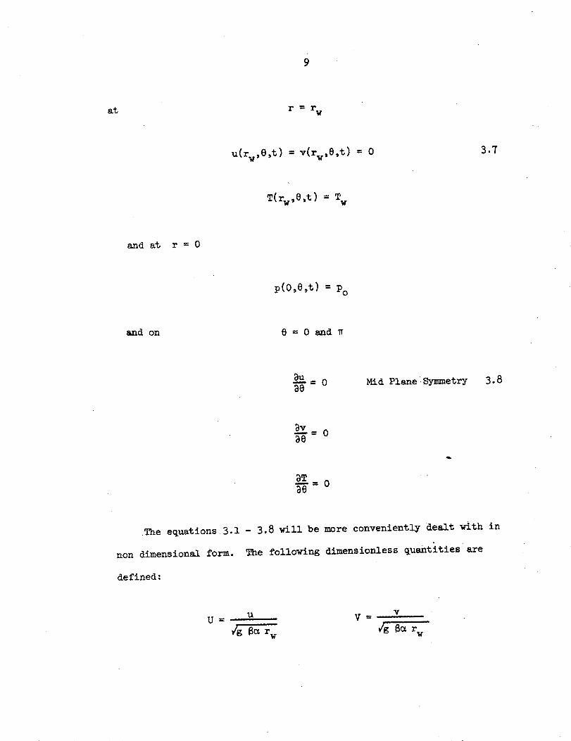
9
r = rw
u(rw,O,t) - v(rw,e,t) = o
T(rw,O,t) = Tw
and at r = 0
p(O,,t) = po
0 = O and n
au =7-8= Mid Plane Symmetry
aTT=
The equations 3.1 - 3.8 will be
non dimensional form. The following
defined:
U = u
'g Ea rw
more conveniently dealt with in
dimensionless quantities are
V = v/g a( rw
at
3.7
and on
3.8
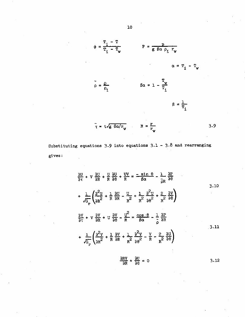
10
g = Pi rwg $ca pi r
= T. -T1 V
TBa = 1 - w
Ti
R = rR- r
=1
Ti
3.9
Substituting equations 3.9 into equations 3.1 - 3.8 and rearranging
gives:
a + vU UU U UV - sin 0+T aR R ae R Ba
+ 2 1/2 + 1 U Uv rG 2 RR aR 2
~~Gr \aR R
+1 a2U
R2 ae2
1 aP
pR ae3.10
+ 2R 1R2 v
+ V + U -DR DeU2 cose' 1 aPR 6a ~ aR
+ av 1 a2vR aR R aDe2
aRV + au = 0aR ae
T. - T
T -T1 w
PiPi
T= t~g 6a/rwV
3.11
3.12
1 ~ a2v
G- \aR
V 2 au2R R2 aeR
11
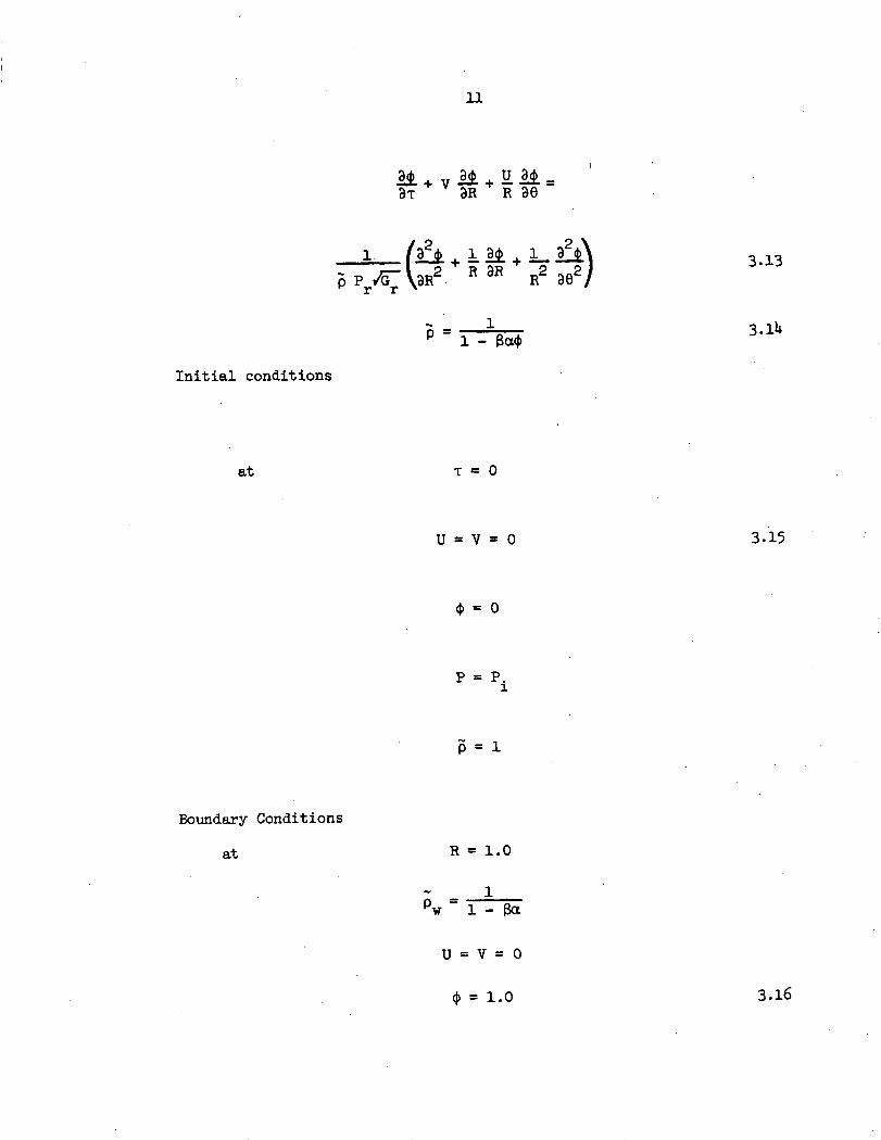
. + v X + u __ =aT aR R ae
+ 1 a R+ 1R DR R2 ae2 /
1P 1- Bam
Initial conditions
T = O
3.15U= V = 0
= 0
P =Pi
Boundary Conditions
R = 1.0
1Pw =1-a
U=V=O
$ = 1.0
3.13
3.14
at
at
1 aP P 3R R2 ,
3.16
12
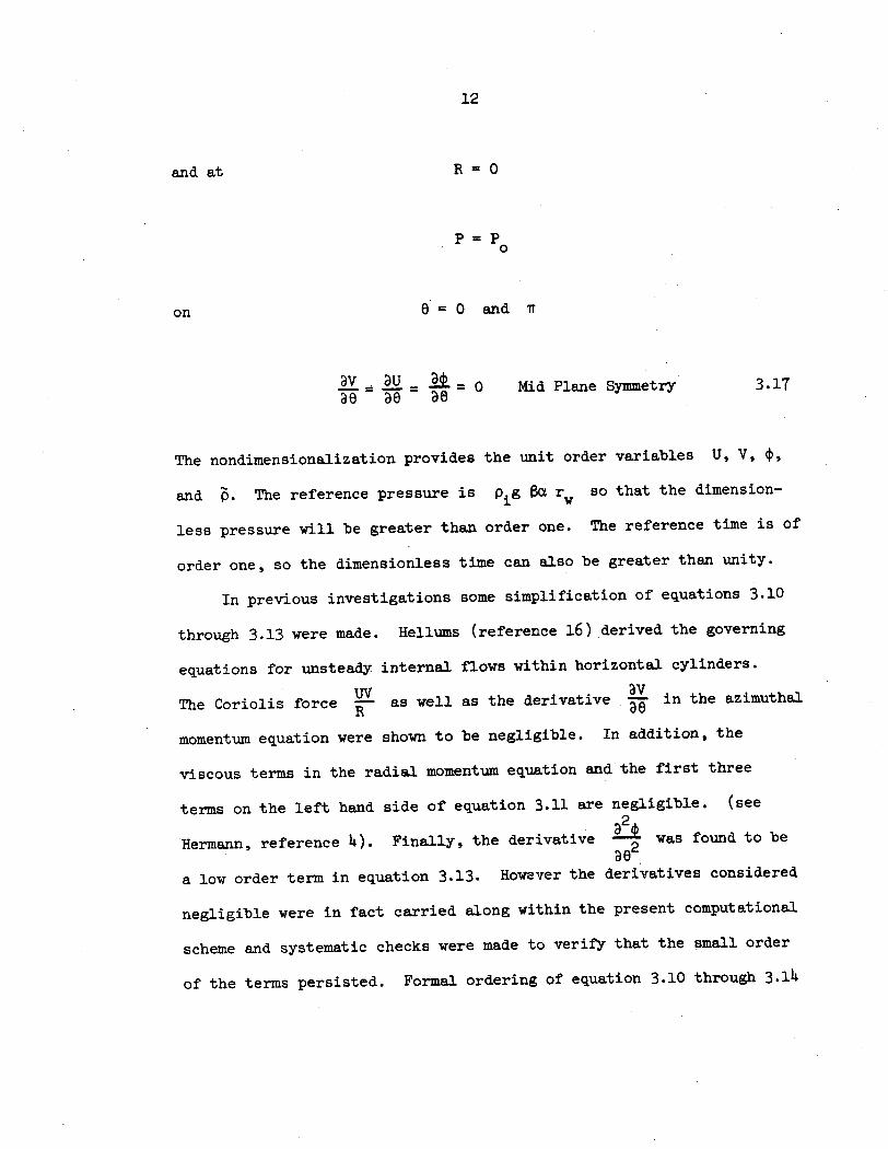
and at R 0
P= P0o
on e =0 and T
av 9 = = 0 Mid Plane Symmetry 3.17
The nondimensionalization provides the unit order variables U, V, *,and p. The reference pressure is pig Oa r
wso that the dimension-
less pressure will be greater than order one. The reference time is of
order one, so the dimensionless time can also be greater than unity.
In previous investigations some simplification of equations 3.10
through 3.13 were made. Hellums (reference 16) derived the governing
equations for unsteady internal flows within horizontal cylinders.
The Coriolis force as well as the derivative aV in the azimuthalR at a
momentum equation were shown to be negligible. In addition, the
viscous terms in the radial momentum equation and the first three
terms on the left hand side of equation 3.11 are negligible. (see
Hermann, reference 4). Finally, the derivative 2 was found to beae
a low order term in equation 3.13. However the derivatives considered
negligible were in fact carried along within the present computational
scheme and systematic checks were made to verify that the small order
of the terms persisted. Formal ordering of equation 3.10 through 3.14
13
by asymptotic series expansions of the dependent variables and stretch-
ing of the normal coordinate is complicated by the eventual thickening
of the boundary layer. At large values of time the boundary layer is no
longer thin and the matched core expansions and inner expansions are
invalidated. An additional simplification to equations 3.10 through
3.14 involves the form of the pressure gradient terms.
It is convenient to divide the pressure into two separate parts:
P = Pi + P * 3.18
Pi is the initial zero motion hydrostatic pressure. P* is a "dynamic"
pressure that arises due to motion and thermal changes within the
fluid. The motivation for equation 3.18 is well founded in that the
initial hydrostatic pressure gradient is known exactly:
1 i sin 3.19p
1 4 i 1 w = = cos e 3.20
For many gravitationally driven flows the contribution to the overall
pressure gradient from De or DR is a small order effect. (see
Hellums reference 16 and Ostrach reference 18). Knowledge of the
hydrostatic pressure gradient facilitates solution of the governing
equations through the use of equations 3.19 and 3.20. With these
considerations and substituting equations 3.19 and 3.20 into equations
14
3.10 through 3.14 the governing system becomes:
+ V + a= - sin 6 _ ( - _a) aYT- BR R M R Be
3.21
+ 1 a2g \aRr
'1 aU U+ B+R 3R R
1a2 u2
R a e2
a.. = -- _ cos 83 R R
aRV au
+ 3R + = 1 o
r r
Initial conditions
T=0
U=V=O
T = 0
P = 0
P* = 0
Boundary conditions
R = 1.0
3.22
3.23
3.24
at
3.25
at
15
U=V=O 3.26
* = 1.0
and at R = O
P* = p*-
and on e = 0 and Tr
aDu= = 0 3.27ae ae
Development of the Finite Difference Approximationto the Governing Equations
Chapter IV
Low velocity fluid flows have proven difficult to solve using
finite difference techniques. When the fluid velocity is low, long
computational times are required, and for gravitationally driven flows
that start from rest, the situation is further aggravated. The fluid
flow studied here should develop maximum velocities on the order of
several feet per second; thus long computational times appear unavoid-
able. The second difficulty arises from the fact that both positive
and negative velocity components may be expected as fluid will be both
entrained and expelled by the boundary layer. Numerical instabilities
are produced by positive and negative coefficients of the convective
terms of a difference scheme unless special care is taken regarding the
form of the differencing. For these reasons an explicit, windward
differencing technique was chosen (also called the donor cell technique).
As shown recently by Roache (reference 19), the windward scheme along
with all but one other scheme (reference 20) have only first-order
accuracy in the transient development of the flow. A diffusive trunca-
tion error is introduced which appears as an artificial viscosity that
may override the physical viscous damping within the fluid. Because of
this, care must be taken with the windward scheme to insure that the
grid size is sufficiently small so that artificial viscous effects do
not have a predominant effect on the numerical development of the flow.
From reference 19 it is seen that the artificial viscosity of the
C
17
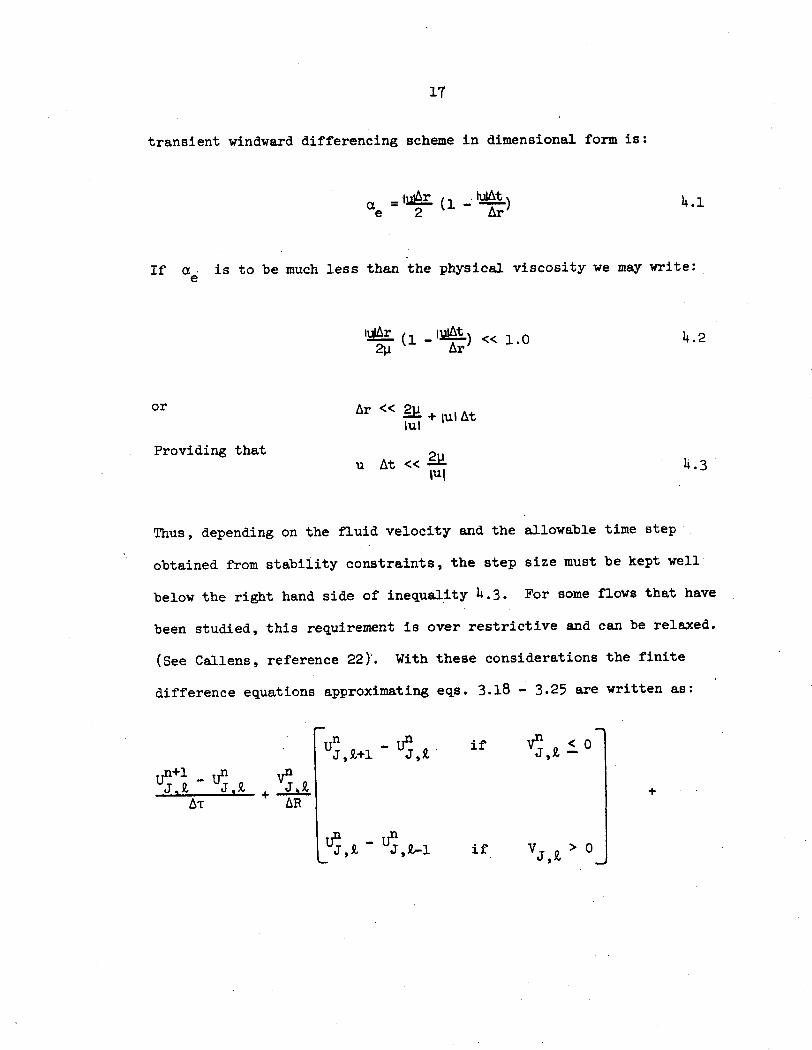
transient windward differencing scheme in dimensional form is:
= IIlUAt 4.~e 2 Ar
If ae is to be much less than the physical viscosity we may write:
1u1r (1 _ ulit) << 1.02o Ar< +A
~~~or Ar << 2 + luAtlul
Providing thatu At << 2P
uuA
Thus, depending on the fluid velocity and the allowable time step
obtained from stability constraints, the step size must be kept well
below the right hand side of inequality 4.3. For some flows that have
been studied, this requirement is over restrictive and can be relaxed.
(See Callens, reference 22)'. With these considerations the finite
difference equations approximating eqs. 3.18 - 3.25 are written as:
n+1 n Vn:
AT Z + Js.-AT AR
UJ,+l1- UJ,Iif Vn <_
J, <0
if V, > 0
1
2
4.3
+
UJ,~- Una,-i
J+l , ,J,
J, - J-1,t
nsin 8 -JIt
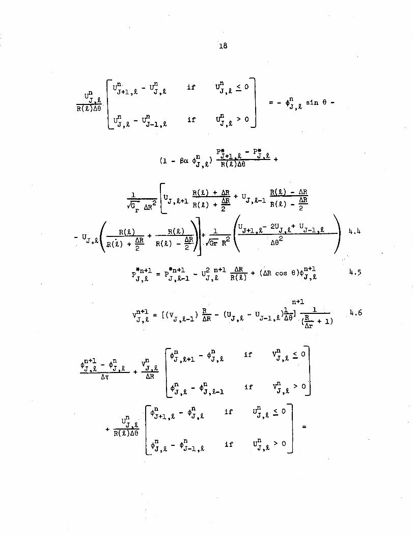
p4*n ) J+l .Z
(1 - 8c gJ, ) R()&e
R(k) + ARAR
R(.) + 2+ U R(Q) - AR
J, R(Q) -
Q + _ R(Q) 01+ 1 tJ+1 - 2Uj ,+ Ui 1 t
AR R(Q) - A .G/ R2 e'22 A
p*n+l n+l _ 2 n+l AR n+
J,k =J,.lR - VJ,k R(-T+ (AR Cos 0,J,k
n+l
JP [(- J,-) - (UJ,t - lUJ_1 -e ]=,R JL-l R (I _ I
4.4
4.5
if U i < 0
iJ >J
if, > 0
ifI
Un
TR3Q4X
J.Q +-- J-~ +
J,+11
V- AR2r
n+l nJ. -iJ,-
AT
vny
+ AR
n n
$J,z+1 - J,
I1X n
$J,Z- 0J,Z-1
Un + Ji
R( Y,)A6
if Un S < 0
J,k --
if Vn < J,. >
if >V"j < 0ifk
n n
.J+i,Z ' J,9
n nJ,Z- ~J-i,
19
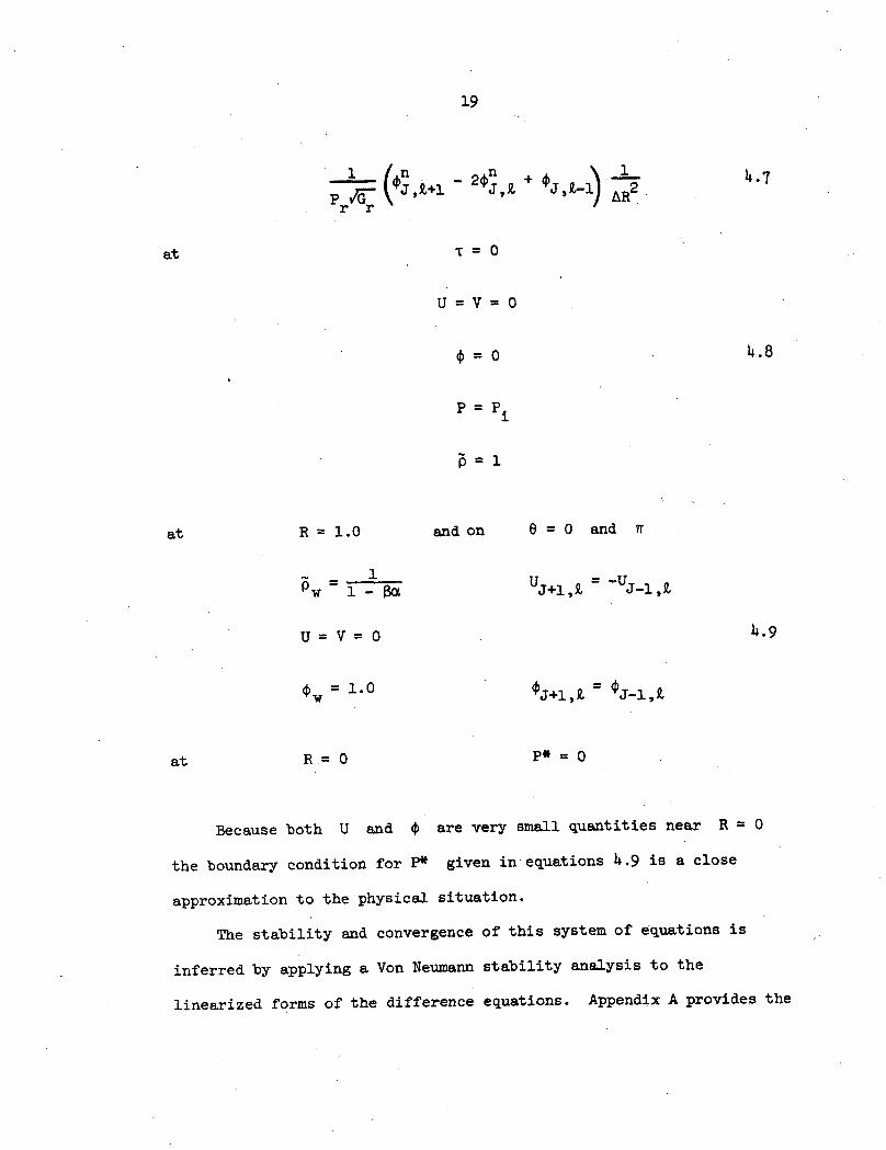
+ J,-1) AR24.7
T= 0
U=V=0
4.8
=Pi
= 1
R = 1.0
1Pw 1 - Baa
U=V=O
w = 1.0
R= 0
and on e =0 and w
UJ+1, =
-UJ-1,
4.9
OJ+1,Z =
J-1,Z
P* = O
Because both U and * are very small quantities near R - 0
the boundary condition for P* given in equations 4.9 is a close
approximation to the physical situation.
The stability and convergence of this system of equations is
inferred by applying a Von Neumann stability analysis to the
linearized forms of the difference equations. Appendix A provides the
at
r nQ 1 r
at
at
20
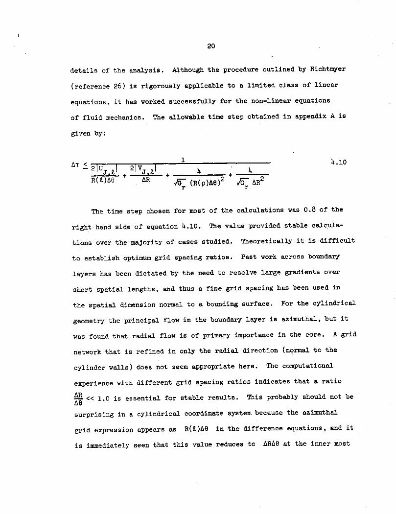
details of the analysis. Although the procedure outlined by Richtmyer
(reference 26) is rigorously applicable to a limited class of linear
equations, it has worked successfully for the non-linear equations
of fluid mechanics. The allowable time step obtained in appendix A is
given by:
- 21|UJ S 21V i 4.10'~a~ne + + 1 +R(.)AO -AR g (R(p)A6) 2 G AR2
r r
The time step chosen for most of the calculations was 0.8 of the
right hand side of equation 4.10. The value provided stable calcula-
tions over the majority of cases studied. Theoretically it is difficult
to establish optimum grid spacing ratios. Past work across boundary
layers has been dictated by the need to resolve large gradients over
short spatial lengths, and thus a fine grid spacing has been used in
the spatial dimension normal to a bounding surface. For the cylindrical
geometry the principal flow in the boundary layer is azimuthal, but it
was found that radial flow is of primary importance in the core. A grid
network that is refined in only the radial direction (normal to the
cylinder walls) does not seem appropriate here. The computational
experience with different grid spacing ratios indicates that a ratio
AR << 1.0 is essential for stable results. This probably should not be
surprising in a cylindrical coordinate system because the azimuthal
grid expression appears as R(L)AO in the difference equations, and it
is immediately seen that this value reduces to ARAE at the inner most
21
grid location next to the origin of coordinates.
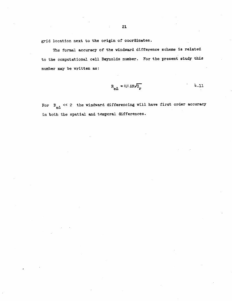
The formal accuracy of the windward difference scheme is related
to the computational cell Reynolds number. For the present study this
number may be written as:
ReA =IUI ARG 4.11
For ReA << 2 the windward differencing will have first order accuracy
in both the spatial and temporal differences.
V Numerical Solutions
A. Constant Wall Temperature
The system of equations 4.4 - 4.9 was solved for values of U, *,
V, and P* over the entire grid following a step-function change in
the cylinder wall temperature at time zero. A flow diagram describing
the calculation sequence is shown in figure 3. It is seen that the
correct difference equations are selected at each grid point depending
upon the sign of Uj,1 or V j, such that stable computations will
result. The program was set up so that computations could be continued
from a previous computer run, and thus extended run times up to 5 hours
on the Langley Research Center CDC 6600 computer were made possible.
Typical computational speeds for a 51 by 31 grid for the half cylinder
were 1.02 x 10⁷ grid points per hour. The real time development of
the flow progressed at a rate of 1.25 seconds per hour of machine time.
An order of magnitude faster flow development time was obtained with a
26 x 16 grid network; however a formal first order accuracy is not
achieved with such a coarse grid.
The steps taken in the computational sequence of events were as
follows:
1. Equation 4.7 was solved over the entire grid for new values
of ~.
2. Equation 4.4 was then solved for new values of U over the
entire grid.
3. Values of $ and U were updated.
22
23
4. Equation 4.6 was solved for the current values of V over the
entire grid.
5. Equation 4.5 was solved for current values of P* over the
entire grid.
6. Values of V and P* were updated.
7. Equation 4.10 was solved to determine an allowable time step.
8. Values of the Nusselt number at the wall were calculated.
The process was repeated over the entire grid for the next time step.
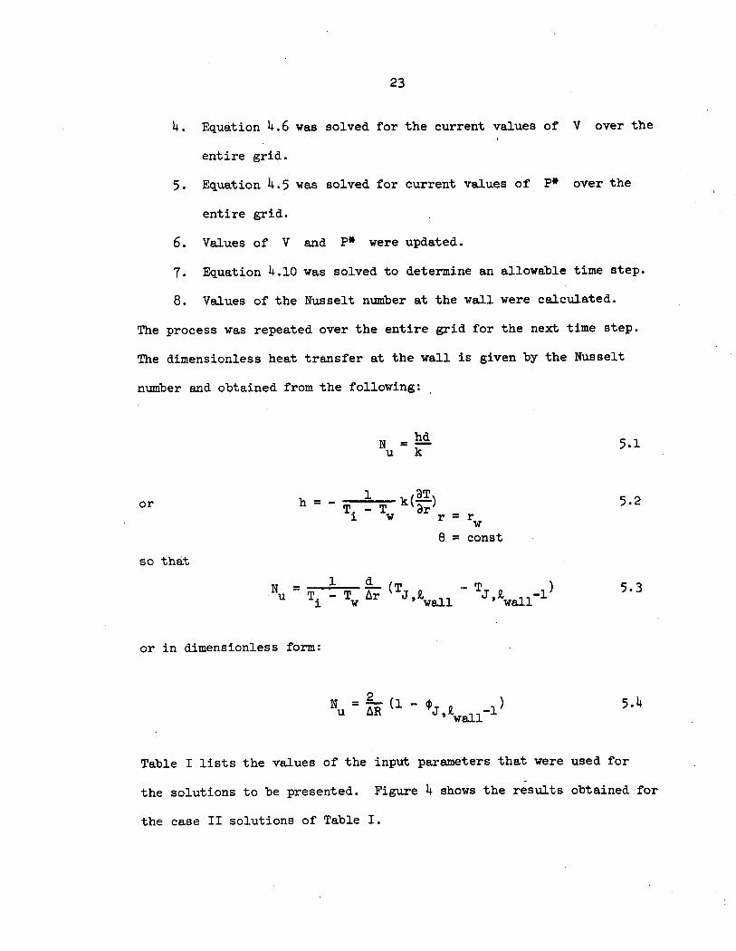
The dimensionless heat transfer at the wall is given by the Nusselt
number and obtained from the following:
N -hd 5.1u k
or h= k( r 5.2Ti w r r
e = const
so that
1 dN -(T -T) 5.3
i Tw wr J wall wall
or in dimensionless form:
N = 2 (1 5.4uwall
Table I lists the values of the input parameters that were used for
the solutions to be presented. Figure 4 shows the results obtained for
the case II solutions of Table I.
From the simple physical geometry of the cylinder a rather compli-
cated flow pattern is revealed by the numerical results. Figure 4a shows
the azimuthal velocity distribution at e = i/2 for three different
time levels. The early time T = 3.05 can be considered as showing the
distribution prior to what is considered to be fully developed flow.
By this it is meant that peak velocities at any given location have not
been achieved. The intermediate time, T = 4.57, shows the velocity
distribution at its peak value, and the late time, T = 14.5, shows the
distribution after a decay in the velocity has taken place. Significant
inward displacement of the peak velocities is not apparent. The
distributions do thicken with time over about 20 grid point spacings,
and the viscous effects are transported further into the core of the
fluid as time progresses. The distributions shown in figure 4 are
typical of all the results obtained for the constant wall temperature
case. Figure 4b shows the velocity distribution near the bottom of
the cylinder at an azimuthal angle of 23.70. The momentum gathered by
the fluid falling downward has both thickened the boundary layer as
well as increased the peak azimuthal velocity. At values of e less
than 230 the fluid rapidly decelerates and comes nearly to rest in
the lower part of the cylinder. Figure 4c shows the velocity distribu-
tion near the top of the cylinder. The boundary layer is well
defined, but the azimuthal velocities are substantially lower than in
the bottom portion of the cylinder near the wall. Figure 5a shows the
radial velocity distribution for case II of Table I. Here it is seen
that the peak velocities are an order of magnitude less than
25
corresponding azimuthal velocities. The radial velocities peak at
their maximum values at the later time, ¶ = 14.5, in contrast to the
azimuthal velocity peaks which occur near T = 4.57. At e = 23.7 ,
figure 5b, the radial velocity is negative which indicates an explusion
of fluid from the boundary layer. As the lower portion of the cylinder
"fills" with fluid that has moved downward in the boundary layer,
negative or radially inward flow takes place to accommodate the added
fluid. Thus, fluid is slowly forced into the boundary layer near the
top of the cylinder due to displacement effects from below. Figure 5c
shows the radial velocity distribution in the upper portion of the
cylinder. At e = 1610 the flow is still developing with peak
velocities occurring near T = 14.5.
Thus the general picture of the flow field involves three major
features. First, there is a boundary-layer development near the wall
due primarily to downward azimuthal fluid flow near the wall. Secondly,
an induced radial velocity occurs that feeds fluid into the developing
boundary layer in the upper and middle azimuthal locations of the
cylinder and ejects fluid out of the boundary-layer at lower azimuthal
locations. Third, a core region exists that strongly resists first-
order motions and only very slowly forces fluid at lower levels to
rise and enter into the boundary-layer. This is a striking example
of a flow in which the principal motion is confined to the boundary
layer.
The dimensionless temperature, T/Ti, is shown as a function of
radial distance in figures 6. Here the thermal-boundary-layer is less
26
well developed than the velocity-layer at a given time. The conduction
terms in the energy equation cause this behavior due to the very low
fluid velocities that occur at early times after the cold wall initial
condition is imposed. The accuracy of the results increases as the grid
network is refined, but the computational time required for fine grids
is enormous. The early behavior of wall-heat transfer is of principle
interest, and figure 7 shows the Nusselt number decay with time for
three different azimuthal stations. The computational results show that
heat is conducted out of the fluid at early times at a greater rate than
energy is convected into a fluid element. As the velocity field
develops, this trend is altered causing a slight steepening of the
temperature gradient near the wall. This result appears to be a valid
physical description of the flow development. The convective terms in
the energy equation are negligible when very low fluid velocities are
present during early times. The result is an energy balance that is
dominated by conduction out of the fluid to the wall until the flow
field develops.
The increasing value of Nusselt number with increasing e gives a
clear picture of the positive upward temperature gradient within the
boundary layer. This positive, upward gradient also exists in the
core fluid as indicated by figure 8. The early establishment of this
upward gradient produces a thermally stable core which tends to resist
downward motion. The low velocities calculated in the core flow are inN
part, a result of this thermal behavior. Figure 9 shows a plot of X
as a function of time. The cold fluid entering and residing in the r
27
lower portion of the cylinder causes a rapid and nearly linear decay
of the dimensionless heat transfer function. For e near w/2 and up
to e = TI, the function decays less rapidly due to the flow of warm
fluid into the boundary layer from the core. At very large times the
heat transfer function must asymptotically approach zero because the
fluid gives up all of its excess energy to the wall. It is apparent
that C1 *+ as T - 0 due to the step function cold wall initial
condition. The actual value of C1 at early times near T = o is
dependent on the radial grid spacing used, as might be expected. A
comparison of the effects of grid refinement is shown in figure 10.
Here the value of T/Ti as a function of radial distance is shown for
three different grid networks. The radial coordinate grid spacings are
.02; .01; and .0067. The azimuthal location is 6 = 90° , and the time
is T = 2.7.
The profiles steepen as the grid is refined and convergence of
the finite difference solution is evident. Of interest is the velocity
distribution shown in figure 10b. Here convergence is also indicated
by the refined grid results. The coarse grid velocity peak is,
however, above the finer grid peaks. The slope of the distributions
near the wall appears to be adjusting itself from an "overshoot" where
AR = .01 to a convergent result as AR becomes smaller. Similar
results have been computed at Grashof numbers of 8 x 10 and 7 x 10⁷
for the grid range given above. Case I of table I was computed for a
Grashof number of 8.3 x 10 . The computational time increases
considerably at this relatively low Grashof number. Figure 11-a shows
28
some representative azimuthal velocity distributions for this case.
The lower Grashof number results for this case can be interpreted as
being due to a more viscous fluid flow, and the distributions reflect
this. At a dimensionless time of T = 3.07 the boundary layer is
considerably thicker than for the comparable boundary layer thickness of
case II. Even at the early time of T = 1.31, the viscous effects are
more pronounced than for the higher Grashof number case. Figure 11-b
shows typical radial velocity distributions for the low Grashof number
case. At T = 3.07 the distribution shows the effects of higher
viscosity with a thicker profile than for the case II solution. Finally,
figure ll-c shows the dimensionless temperature function distribution.
Again the more viscous fluid of case I shows a thicker thermal
boundary layer than the case II solution. All of the profiles for case
I have a qualitative resemblance to the results for case II. The lower
Grashof number solutions for the Nusselt-Grashof relation are shown in
figure ll-d. These curves should be compared with the results shown
in figure 9.
The computations for the dimensionless dynamic pressure, P*,
indicate that the dynamic pressure gradient makes only a small order
contribution to the momentum balance within the fluid. This occurrence
is consistent with the results reported by Ostrach in reference 18 and
24.
The results of the computations for case III at a Grashof number
of 1.3 x 10⁶ are shown in figure 12. The velocity profiles and
temperature profiles represent a result that is intermediate to the case
29
I and case II solutions.
B. Time Varying Wall Temperature
Comparison of the experiments to be described in Chapter VI with
numerical solutions necessitated the use of a time-dependent wall
temperature boundary condition. The experimental wall temperature
decay can be described by solution to the one-dimensional heat conduc-
tion equation. For a wall of thickness x initially at a temperature
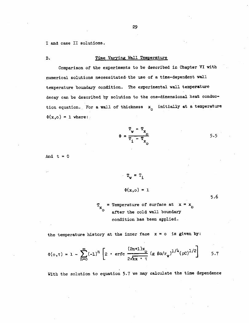
O(x,o) = 1 where:
T -Tw x
T= o 5-5Ti - T
0
And t = 0
Tw = Ti
(x,o) = 1
5.6
T = Temperature of surface at x = xX o
after the cold wall boundary
condition has been applied.
the temperature history at the inner face x = o is given by:
co·I2 (2n+l)xo r w
O) = n(-lo )n [2 * erfc °- (g aC/r )/4(PC)'/2] 5.7n=o 2&XX · T
With the solution to equation 5.7 we may calculate the time dependence
30
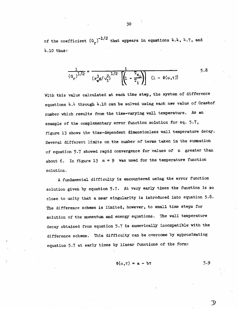
of the coefficient (Gr)-l / that appears in equations 4.4, 4.7, and
4.10 thus:
115.8
(G r) 3 2 1/2,) .Tl (1 - ( - ,T))
With this value calculated at each time step, the system of difference
equations 4.4 through 4.10 can be solved using each new value of Grashof
number which results from the time-varying wall temperature. As an
example of the complementary error function solution for eq. 5.7,
figure 13 shows the time-dependent dimensionless wall temperature decay.
Several different limits on the number of terms taken in the summation
of equation 5.7 showed rapid convergence for values of n greater than
about 6. In figure 13 n = 9 was used for the temperature function
solution.
A fundamental difficulty is encountered using the error function
solution given by equation 5.7. At very early times the function is so
close to unity that a near singularity is introduced into equation 5.8.
The difference scheme is limited, however, to small time steps for
solution of the momentum and energy equations. The wall temperature
decay obtained from equation 5.7 is numerically incompatible with the
difference scheme. This difficulty can be overcome by approximating
equation 5.7 at early times by linear functions of the form:
(o,T) = a - bT 5.9
Di
31
An approximation to the error function solution can be made using
equation 5.9 if we choose: a 4 0.99 and b = 0.050. Figure 14 shows
the azimuthal velocity distribution for the case where the wall
temperature decays according to equation 5.9 rearranged:
Tw = b(OT)(Ti TX ) + Tx 5.100 X0
The results shown in this figure correspond to the case II input values
of Table I.
The time-dependent wall temperature solutions exhibit several
interesting differences from the constant wall temperature solutions.
In effect, a slowly cooled wall-boundary condition produces an early
time driving force that is quite small. This is characterized by the
time development of the Grashof number. Figure 15 shows a typical time
history of the Grashof number for the case II input values and a wall
that follows a temperature history given by equations 5.9 and 5.10.
The development of the flow field is directly related to the time
dependent Grashof number. The immediate consequence of a slowly cooled
wall should appear as a less fully developed flow at any given time than
one for which a step function wall temperature change has been imposed.
The early time behavior is closely related to a lower Grashof number
flow field. The boundary layer development follows the rising Grashof
number with a different behavior than for the constant wall temperature
results. In effect the driving force increases with time, and thus
the flow experiences a longer and more pronounced acceleration. Figure
32
16-a shows a typical temperature distribution for the time-dependent
wall boundary condition as well as for the constant wall temperature
case. The 'details revealed by these curves are physically valid in
that the constant wall temperature case, of necessity, must have a
steeper slope near the wall and, in addition, must have a thinner
thermal boundary layer due to the higher Grashof number at equal
values of time. These features are clearly evident in figure 16-a.
A comparison of the constant and variable wall temperature cases
at equal values of the Grashof number reveals the fundamental differences
between the two cases. Figure 16-b shows that the variable wall
temperature still has the effect of producing a more viscous flow
by maintaining lower Grashof numbers throughout the entire time
development than the constant cold wall case maintains. A comparison
with the constant Grashof number case is difficult because of the
fundamental difference between the two case histories. If the two
boundary layer thicknesses are compared at equal values of R and
time, we find the results shown in figure 17-a. The difference in the
peak values of the dimensional velocity are.of course even greater than
shown in this figure because of the different value of reference velocity
used in the non-dimensionalization, i.e. u =-g Oa rw
U. A
comparison of the dimensionless azimuthal velocity distributions at
equal values of both Grashof number and time is shown in figure 17-b.
As expected the time varying wall case shows a thicker profile but
with lower peak velocities. Similar results were observed for the
temperature distribution which is also an indirect result of the
33
viscous behavior of the fluid. Perhaps the most significant single
consideration regarding the energy transfer to the walls is the time
dependent Nusselt-Grashof correlation. Hellums (reference 16)
established the constant C in the relation N = C G1 /4 . Foru r
steady flow within a horizontal cylinder C = 0.326. If a fully
developed flow occurs in the present problem, the time dependent C(T)
should approach the steady value prior to a decay in the fluid motion.
As time increases indefinitely in the present unsteady flow, C (T) 4
o, since the fluid will then have given up all its excess energy to the
cold walls. Figure 18 shows the time-dependent behavior for the Nusselt-
Grashof correlation. The relation N /G1/4 is seen to rapidly approachIu r
the steady state or fully developed value. The unsteady flow value of
this relation for the present problem must be asymptotic with zero at
large values of time. This behavior is demonstrated by the numerical
results represented in figure 18.
Figures 19-a through 19-d illustrate the time history of "fluid
particles" within the flow field from a sequence of photographs which
were taken from an oscilloscope display of the particle displacements as
computed from the numerical solutions. As shown in these figures par-
ticles were located, at t = 0, along rays separated by an azimuthal dis-
tance of w/8. From R = 0 to R = .64 the particles were spaced radially
with AR = .04. From R = .64 to R = 1.0 the radial spacing was AR = .01.
A two dimensional interpolation was used to obtain particle displacements
between grid locations for the 31 by 101 mesh used for this case. The
time dependent wall temperature decay for case II-T of table I was used.
The sequence of photographs shows the fluid deceleration and strati-
fication near the bottom of the cylinder. Regions where the number of
particles increase represent regions of higher fluid density as might
be expected. Figure 19-e is a plot of the displacements at 6.6
seconds. In this figure the particles belonging to each original ray
have been faired in to illustrate the displacement profiles. Real
time movies were made from plots such as these to give a physical
picture of the flow field development. Because of the low velocities
within the core flow, large values of time must be obtained with the
numerical solutions before substantial particle displacements can be
observed within the core.
Chapter VI - EXPERIMENTAL STUDIES
Apparatus
The instrumented stainless steel cylinder used for measuring
temperature distributions in a gravitationally driven flow field is
shown in figure 20-a. Experiments were made with the cylinder in a
horizontal position, and rotation of the cylinder allowed measurements
to be made at different azimuthal locations. Gage marks and internal
thermocouple probes were used as references in setting the cylinder
in a desired position, and a positive lock cradle was made to insure
that the cylinder maintained a given position. An optical transit was
used for precise orientation of the entire system. Figure 20-b is a
schematic diagram of the entire apparatus. The cylinder was made of
schedule 40 non magnetic stainless pipe with 300 series stainless steel
end caps welded in place. The inside diameter was nominally 5.94
inches and the length was 60 inches. The cooling manifolds were
insulated from the outer cooling Jacket by means of one inch thick
micarta rings. The purpose of this insulation was to allow filling of
the coolant tanks prior to a run, and cooling the liquid to a uniform
temperature without introducing conduction effects downward to the
actual test cylinder. A threaded connection between the outer Jacket
and the test cylinder established a conduction path that had to be
accounted for, and thus the insulator rings were installed.
The inside surface of the test cylinder was machined to a smooth
finish with average surface projections not greater than 220 micro
35
36
inches from peak to valley. The cylinder was cleaned and vacuum leak
tested prior to installation of the instrumentation. The cylinder
maintained a pressure of less than 10' 6
mm of mercury for a 24 hour
period.
Figure 21 is a photograph of the cooling tanks, inlet manifolds,
and outer' cooling Jacket surrounding the test cylinder. The valves
for dumping the cooling fluid into the outer cooling Jacket were
manually operated, and the liquid coolant in the tanks could be
completely discharged in less than one second. The "o" ring sealed
valves shown in figure 20-b proved exceptionally reliable, and because
of their large size the effective discharge rate from the coolant tanks
was in excess of 2500 gallons per minute.
Instrumentation
Two sets of thermocouple probes were installed through the walls
of the test cylinder. Initially copper-constantan thermocouple probes
were installed as shown in figure 20-b for the purpose of determining
whether or not a region of two dimensional flow existed in the region
away from the end walls. Near the mid section of the cylinder there
appeared to be no end wall effects and the thermal field was two
dimensional.
The cylinder was then instrumented with a series of thermocouple
probes to measure temperatures across the boundary layer at an l/d = 5.
The baundary-layer probes were made from 30 gage copper-constantan
wire with fiber sheathing left on the probes to reduce axial-conduction
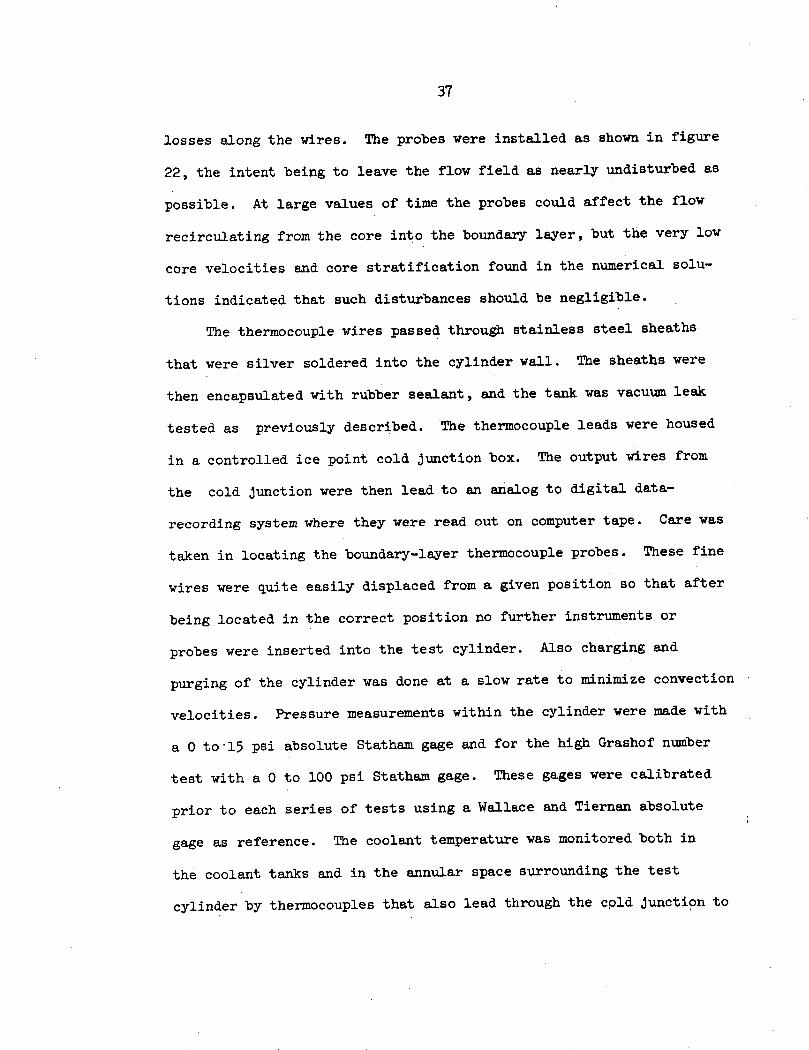
37
losses along the wires. The probes were installed as shown in figure
22, the intent being to leave the flow field as nearly undisturbed as
possible. At large values of time the probes could affect the flow
recirculating from the core into the boundary layer, but the very low
core velocities and core stratification found in the numerical solu-
tions indicated that such disturbances should be negligible.
The thermocouple wires passed through stainless steel sheaths
that were silver soldered into the cylinder wall. The sheaths were
then encapsulated with rubber sealant, and the tank was vacuum leak
tested as previously described. The thermocouple leads were housed
in a controlled ice point cold Junction box. The output wires from
the cold Junction were then lead to an analog to digital data-
recording system where they were read out on computer tape. Care was
taken in locating the boundary-layer thermocouple probes. These fine
wires were quite easily displaced from a given position so that after
being located in the correct position no further instruments or
probes were inserted into the test cylinder. Also charging and
purging of the cylinder was done at a slow rate to minimize convection
velocities. Pressure measurements within the cylinder were made with
a 0 to 15 psi absolute Statham gage and for the high Grashof number
test with a 0 to 100 psi Statham gage. These gages were calibrated
prior to each series of tests using a Wallace and Tiernan absolute
gage as reference. The coolant temperature was monitored both in
the coolant tanks and in the annular space surrounding the test
cylinder by thermocouples that also lead through the cold Junction to
38
the data recording system.
Test Procedure
The test procedure consisted of charging the cylinder with dry
air at ambient temperature, sealing off the inlet and outlet valves to
the cylinder, and then allowing a two hour waiting period for convec-
tion currents to damp out within the cylinder. Thirty minutes prior
to a test, water and cracked ice were introduced into the coolant
tanks, and the coolant was brought to a uniform and steady temperature
that typically was 4940 R. With all thermocouples displaying steady
state readings the plug valves were opened, and the coolant was dumped
over the test cylinder walls. Immediately upon opening the plug
valves, a circulating pump was activated to minimize temperature
gradients in the cold liquid by drawing cold liquid out of the
annular region surrounding the test cylinder, and spraying the coolant
back over the ice crystals in the coolant tanks. Strainers at the
bottom of each tank prevented solid ice from going past the plug
valves and into the annular tank chamber.
For a period of approximately five minutes following the coolant
dumping, data sampling of all thermocouples and pressure instrumen-
tation was taken. The digital system sampled each channel 400 times
per second and stored the values on tape. A printer output from the
digital system gave separate channel print outs at a rate of about 5
channels per second for convenience in visually following the temperature
and pressure changes from the digital system.
39
Following a test, the coolant was removed from the system and room
temperature water was flushed through the coolant tanks, valves, and
annular chamber. Dry, ambient air was pumped through the test cylinder
and it was sealed off when all thermocouple readings showed steady,
ambient temperatures existed within the cylinder. A two hour waiting
period, was then used as previously described.
Two series of tests were made using Freon and dry ice as the
coolant. Wall temperatures down to 4000 R were achieved but it was found
almost impossible to maintain uniform coolant temperatures. The problem
was due to the formation of "snow" when dry ice was sublimed in Freon.
A more reliable approach for raising the Grashof number was taken by
pressurizing the cylinder. The experimental data reported here was
obtained at a nearly constant gas to final wall temperature ratio ofTw = .936.
T.1
Attempts to Measure Gas Velocities
Considerable effort was put into an attempt to measure gas velo-
cities near a wall in natural convection flow. Early studies by
Martini and Churchill (reference 17) using titanium dioxide dust were
difficult and with considerable uncertainty. The attempt made here
involved the use of helium filled soap bubbles. A flat plate was
constructed to test against previous experiments and theory. This
plate is shown housed in a plexiglass cage in figures 23-a and 23-b.
At time zero hot water was forced through three passages internal to
the plate. At the same time, bubbles that were filled with mixtures of
40
He and N2 and were neutrally buoyant were introduced to the lower
leading edge region of the plate. Color movies were taken of the rapid
entrainment of the bubbles into the plate boundary layer, and their
subsequent acceleration vertically upward. Time displacement studies
were made of the bubbles. Almost independent of bubble size, the bubbles
all seek out a single streamline in the plate boundary layer. Thus it
appears nearly impossible to measure a velocity profile. The reasoning
for why the bubbles behave in this manner is based on the fact that the
boundary layer is quite thin for the plate tested, and thus a steep
velocity gradient normal to the plate exists which in effect produces
a gradient across the bubble. Such a velocity gradient would act to
draw the bubble laterally inward to a position of peak velocity within
the boundary layer. A comparison of the measured velocities for both
transient and steady flow conditions indicated that the bubbles were in
fact traveling with close to the maximum theoretical velocities deter-
mined by Siegel (reference 25). The solution to the difficulty appears
to be in producing a very thick boundary layer such that the bubble
size is small compared to the change in velocity across a distance of
one bubble diameter. Extensive tests were made to produce extremely
small bubbles but below about .05 inches diameter neutral buoyancy
cannot be achieved at standard atmospheric conditions. The hope of
mapping out the velocity distribution within the cylinder by tracing
the bubble displacements had to be abandoned.
Discussion of the Experimental Results
Chapter VII
Comparison of the numerical results and the experiments necessitated
a consistent formulation of both the dimensionless variables as well as
identical wall boundary conditions. Also the numerical solutions must
have the initial conditions imposed at the same time zero as actually
occurred in the experiments. It was found that within 0.4 sec after
application of the cold liquid to the cylinder wall, temperature drops
were detected within the gas near the wall. Thus time zero could be
determined within 0.4 second by thermocouple signals alone. For
comparison with the numerical results, the heat conduction equation was
used for determining time zero for the experiments by allowing time
zero for the conduction problem to occur when the liquid was first
dumped from the hoppers. Time zero for the numerical computations and
the fluid was taken when a 0.2 Rankine decrease in wall temperature
had occurred due to conduction. (See equation 5.9)
1As discussed in chapter 5, the near singularity in for a
Grtime dependent wall temperature, limits the value of the constant, a,
in equation 5.9 to values less than about .99.
With these considerations the measured and computed temperature
distributions for an azimuthal angle of 900 are shown in figure 24.
These results correspond to case II of table I with the exception of
a variable wall temperature as mentioned above. The numerical solutions
for 1.2, 4.0, and 8.0 seconds of real time compare favorably with the
41
42
measured results. The large computing time for the program prohibits
carrying out the numerical solutions to larger values of time. The
gradual thickening of the thermal boundary-layer is seen in these
figures. Because the core acts as a reservoir of warm fluid for supply-
ing the boundary layer, the temperature distributions within the layer
tend to retain their profiles over a long period of time after the
velocity field starts decaying. To illustrate the temperature decay,
figures 25 show typical plots of both the experimental and theoretical
temperature at a selected radial location. Figure 25-a shows an early
time behavior both from experimental measurements, and from the numerical
solutions that clearly indicates the inflection produced by the flow as
the velocity distribution shifts toward a more developed profile.
Similar behavior is seen in figure 25-b at 8 = 70° . Finally at the
bottom of the cylinder where the azimuthal motion of the fluid ceases,
the temperature decay appears as shown in figure 25-c. The numerical
results predict a more rapid decay than was actually measured. Several
possible reasons for the disagreement are available. The most likely
source of error lies within the framework of the differencing scheme
near the mid-plane of symmetry. Because both the azimuthal and radial
velocities are negative near the bottom of the cylinder, forward
differencing is used throughout the momentum and energy equations. But
forward differencing carries the grid points into regions of largest
change and tends not to balance with the backward grid points that,
for the present physical system, lie in regions of lesser change. Near
the mid-plane the azimuthal velocity goes to zero but forward differencing
tends to override this due in part to the finite grid size, and thus it
appears that errors may be largest near the bottom mid-plane of symmetry.
In this respect the solutions are dependent upon the cylindrical geo-
metry being considered. This represents a limitation or at least an
undesirable aspect of one sided finite difference techniques.
It is of some interest to observe the experimentally measured
pressure decay within the cylinder. This decay represents a three-
dimensional (closed volume) phenomenon that is in a sense primarily
dependent on the two-dimensional flow field that transports heat to the
cylinder walls. Figure 26 shows a typical measured pressure decay for
the case of a maximum Grashof number of 7 x 10⁷. The pressure decay
is a direct measure of the over all energy loss from the fluid.
The mass in the enclosed cylinder remains constant over the total
volume and thus values of the average tank pressure are a function of
the average fluid temperature within the cylinder.
The single most important comparison made between the numerical
results and the experiments is that of the Nusselt-Grashof relation
for the time dependent flow. Figure 27 shows the measured time
dependent variation of this dimensionless grouping. The comparison is
favorable. Many steady state natural convection flows can be described
by the Nusselt-Grashof correlation and from figure 27 it appears that
a time dependent correlation could be written for an internal flow
with the boundary conditions presently under consideration. The
formulation of such a relation was not attempted in this study.
44
The Nusselt-Grashof relation is asymptotic with zero at large
time as seen by:
Gr1/4 rwg i - Tw
2 i d
When 'T * J we find 1 and the right hand side of equation 7-1
goes to zero. The value of NU/Gr/4 will pass through Hellum's steady
state value (0.326) about 14 seconds after initiation of the flow.
If figure 27 is compared to figure 18 the effect of a steadily decaying
wall temperature is apparent. The curve shown in figure 27 can be
interpreted as being a result of lower values of heat transfer when the
wall is cooled unsteadily than when a step function cold wall is applied,
such as for the figure 18 conditions.
Examples of typical experimental radial temperature distributions
are shown in figure 28. In figure 28a at t = 4.0 seconds, the wall
has cooled to about .983 of the initial temperature, and thus the
distribution terminates at the wall (R=1.0) in the manner shown.
The thermocouple located at R = 0.2 was considered essential for
monitoring the core temperature. If a very low ratio of Tw/Ti had
been utilized, it could be anticipated that fluid would fall downward
from the upper most walls of the cylinder. In such a case a negative
vertical temperature distribution within the core might have been
45
observed. For the Tw/Ti
ratio of these experiments the flow was
almost completely confined within the wall boundary layers, and no
negative upward distributions were measured. Figure 28-b shows the
temperature distribution at 8.0 seconds after flow initiation. The
measured profile has broadened more than the numerical solutions
predict. Figure 29-a shows a similar result for e = 700.
A series of experiments at Grashof number values up to about
1.8 x 10 were made and some results are shown in figures 30. The
very slow time development of the flow field is indicated by both the
numerical calculations which take almost an order of magnitude longer
computational time, than the case II solutions and by the experiments.
The agreement between the numerical solutions and the experiments is not
as good at low values of the Grashof number as at the higher Grashof
numbers. The very slow development of the flow reduces the early time
accuracy because of the small differences in temperature that must be
measured. Figure 31 is a plot of the time history of the boundary-
layer temperature at R = .966. The slow decay is an example of the
lower Grashof number behavior. However, the relatively more rapid
reduction of the gas to wall temperature ratio for the lower Grashof
number case produces an undershoot of the Nusselt-Grashof relation.
This is due to the differences between the velocity field development
and the thermal field development and is shown in figure 32. An
initial response to the near singularity at early times due to low
values of the Grashof number causes the undershoot in the numerical
results. Thus although the disturbance is damped by the difference
scheme, the accuracy of the results is severely lessened by the
destabilizing influence of a very low early time Grashof number. Re-
stated, the low Grashof number computations are characterized by a
relatively rapid wall cooling which raises the wall heat transfer more
rapidly than the one fourth power of the Grashof number. The Nusselt-
Grashof behavior in both figure 27 and figure 32 must be viewed as
being representative of one specific flow configuration, and also a
very specific boundary condition. The difference between figures 27
and 32 indicates that a single correlation equation from the numerical
results presented here, may not be possible to achieve for the entire
range of unsteady laminar natural convection flow within a horizontal
cylinder.
Conclusions
Chapter VIII
The present investigation has revealed the dynamic and thermal
behavior of a confined fluid subjected to gravitational body forces.
For a semi-infinite horizontal cylinder with uniformly cold walls the
principle features of the flow involve a rapid development of the
boundary layer adjacent to the walls, a tendency for fluid stratifica-
tion in the lower regions of the cylinder, and a slow decay of the
velocity and thermal fields with time. Experiments made in this
investigation substantiate the thermal behavior predicted by numerical
solutions to the quasi-compressible Navier-Stokes equations for the case
of a time dependent wall temperature decay. Because the thermal and
velocity fields are strongly coupled, the experimental findings imply
that the velocity field may also be accurately described by the
numerical results.
The following conclusions can be drawn from this study:
1. For very low velocity natural convection flows, windward
finite differencing, which gives first order accuracy in time and space,
is a suitable numerical scheme when positive and negative velocities
occur. The large computing times required for such flow fields rules
out more time consuming differencing schemes at the present time.
2. The windward scheme in cylindrical coordinates was not
extremely sensitive to grid spacing ratios except when the ratio
ARA 0.2. Above this value, numerical instabilities occurred regardless
of the time step used.
3. The differencing scheme appeared to lose accuracy near the
bottom of the cylinder where both the radial and azimuthal velocities
are negative, and the azimuthal velocity is decelerating to zero at
e = 0.
4. The early establishment of a positive upward temperature
gradient within the central core flow, along with the effects of fluid
viscosity combine to produce a strong resistance to induced fluid
motion within the core. After initiation, the flow within the
boundary layer develops rapidly, and decays over a long period of time.
5. The dynamic pressure gradient terms 1 BP and BR are
negligible in the azimuthal and radial momentum equations for the
conditions considered in this investigation.
6. The relationship between the Nusselt and Grashof numbers is
found both numerically and experimentally for the case of unsteady
natural convection flow within a horizontal cylinder subjected to
uniformly cold wall boundary conditions. For the case of a time
dependent wall boundary condition, the Nusselt-Grashof relation inter-
cepts the steady state value of the dimensionless group about 14
seconds after the commencement of flow down the cylinder walls. For
the case of a constant cold wall condition from time zero, the numerical
results show that the Nusselt-Grashof relation intercepts the steady
state value at about 3 second after commencement of the flow.
7. No first order vortical motion was found within the core flow.
The absence of this motion is attributed to the boundary conditions
49
which require azimuthal deceleration of the boundary layer flow near
the bottom of the cylinder. Both the theoretical and experimental
models establish a mid plane of symmetry that satisfies the boundary
conditions imposed in this study.
Bibliography
1. Nusselt, W.: Gesundh. Ing., Bd. 38, 1915.
2. Hermann, E.: Phys. Zeichshrift Bd. 33. 1932.
3. Beckmann, W.: Forsch Ing.-Wes., Bd. 2 1931.
4. Hermann, R.: Heat Transfer by Free Convection from HorizontalCylinders in Diatomic Gases, NACA TM-1366 1954 (Translation).
5. Wamsler, F.: VDI Forschungsheft. 98/99 (Berlin) 1911.
6. Koch, W.: Beih. z. Gesundh.-Ing. Reihe 1, Heft 22 1927.
7. Jodlbauer, K.: Forsch. Ing.-Wes., Bd. 4 1933.
8. Ostrach, S.: Laminar Natural Convection Flow and Heat Transfer ofFluids with and without Heat Sources in Channels with ConstantWall Temperatures NACA TN-2863 1952.
9. Lewis, J. A.: Free Convection in Commercial Insulating MaterialsPh. d. Thesis, Brown University Providence, R. I. 1950.
10. Batchelor, G. K.: Heat Transfer by Free Convection across aClosed Cavity between Vertical Boundaries at DifferentTemperatures. Quart. Journ. of Appl. Math. 12 209 1954.
11. Pillow, A. F.: The Free Convection Cell in Two Dimensions, AeroResearch Lab. Dept. A-79 1952, Melbourne, Australia.
12. de Vahl Davis, G.: Laminar Natural Convection in a RectangularCavity, New York University, School of Eng. Report No. F-67-21967.
13. Weinbaum, S.: Natural Convection in a Horizontal Cylinder, Journ.of Fluid Mechanics, 18, 409 1964.
14. Menold, E.: Natural Convection in a Horizontal Cylinder at LargePrandtl Numbers, Case Institute of Technology, Ph.d Thesis, 1966.
15. Hantman, R. G.; Ostrach, S.: Natural Convection inside aHorizontal Cylinder, AFOSR Scientific Report AFOSR68-2341 1969.
16. Hellums, J. D.: Finite Difference Computation of NaturalConvection Heat Transfer, Ph. d. Thesis University of Michigan,1961.
50
51
17. Martini, W. R.; Churchill, S. W.: Natural Convection inside aHorizontal Cylinder, American Institute of Chemical EngineersJ. 6. 251,1960.
18. Ostrach, S.: Laminar Flows with Body Forces, The Theory ofLaminar Flows, Ed. F. K. Moore, Princeton University Press,Princeton New Jersey, 1964.
19. Roache, P. J.: On Artificial Viscosity Sandia Research ReportSC-PR-71-0301, 1971.
20. Lax, P. D.; Wendroff, B.: Systems of Conservation Laws, Communica-tions on Pure and Applied Mathematics Vol. 13, 217-237, 1960.
21. Brooks, I. H.; Ostrach, S.: An Experimental Investigation ofNatural Convection in a Horizontal Cylinder, AFOSR ScientificReport., TR-69-0174, 1969.
22. Callens, E. E. Jr.: A Time Dependent Approach to Fluid MechanicalPhenomenology, AIAA Paper 70-46, January 1, 1970.
23. McAdams, W. H.: Heat Transmission 3rd Ed. McGraw-Hill 1954.
24. Ostrach, S.: An Analysis of Laminar Free Convection Flow and HeatTransfer about a Flat Plate Parallel to the Direction of theGenerating Body Force. NACA Report 1111, 1953.
25. Siegel, R.: Transient Free Convection from a Vertical Flat PlateTransactions of the ASME Vol. 80 No. 2 February 1958.
26. Richtmyer, R. D.: Difference Methods for Initial Value ProblemsInterscience Publishers, 1957.
27. Moffat, R. J.: Gas Temperature Measurement in Temperature itsMeasurement and Control Science and Industry Vol. 3 Part 2C. M. Herzfeld Ed. Reinhold Corp. 1962.
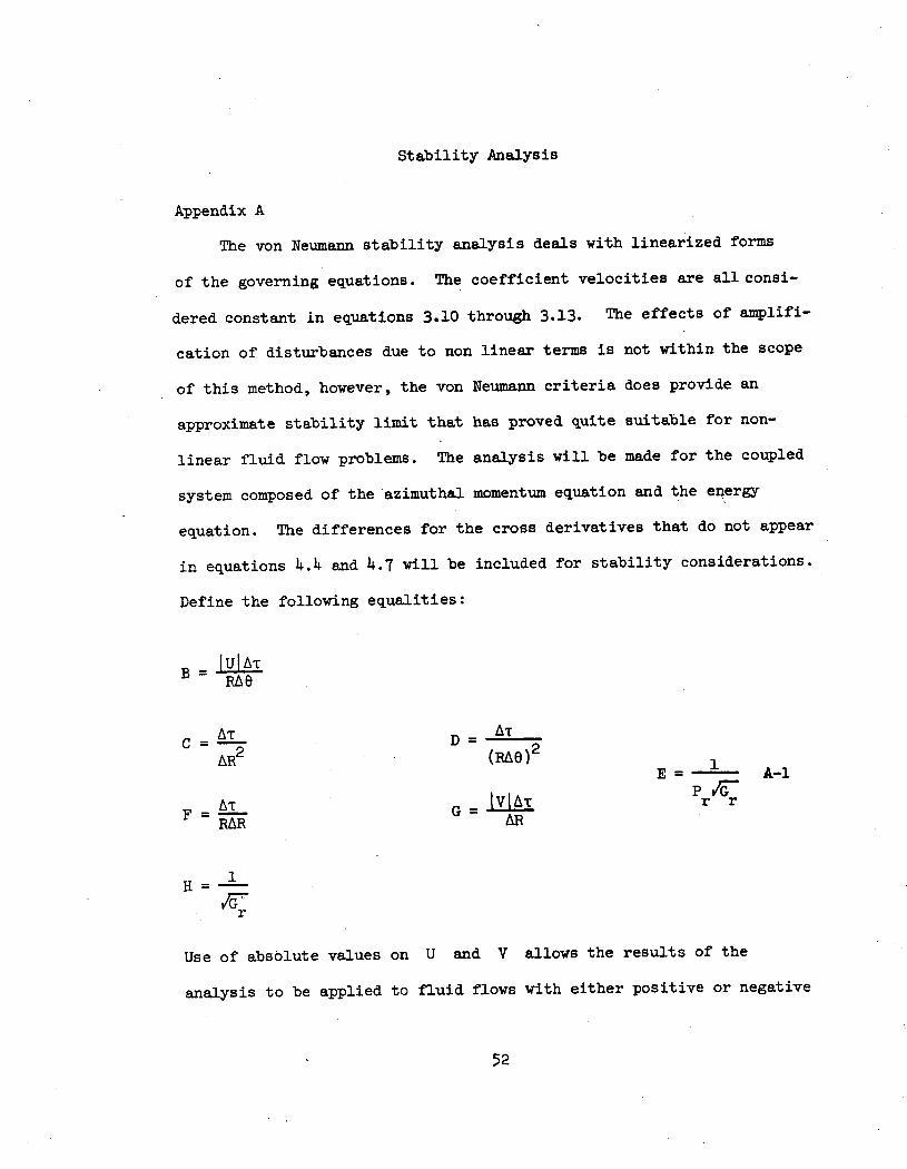
Stability Analysis
Appendix A
The von Neumann stability analysis deals with linearized forms
of the governing equations. The coefficient velocities are all consi-
dered constant in equations 3.10 through 3.13. The effects of amplifi-
cation of disturbances due to non linear terms is not within the scope
of this method, however, the von Neumann criteria does provide an
approximate stability limit that has proved quite suitable for non-
linear fluid flow problems. The analysis will be made for the coupled
system composed of the azimuthal momentum equation and the energy
equation. The differences for the cross derivatives that do not appear
in equations 4.4 and 4.7 will be included for stability considerations.
Define the following equalities:
B = IUIATRAQ
C= D=AR
2(RAe)2 1
E =- A-1
__T IVIAr r rFRAR G = AR
1H=
r
Use of absolute values on U and V allows the results of the
analysis to be applied to fluid flows with either positive or negative
52
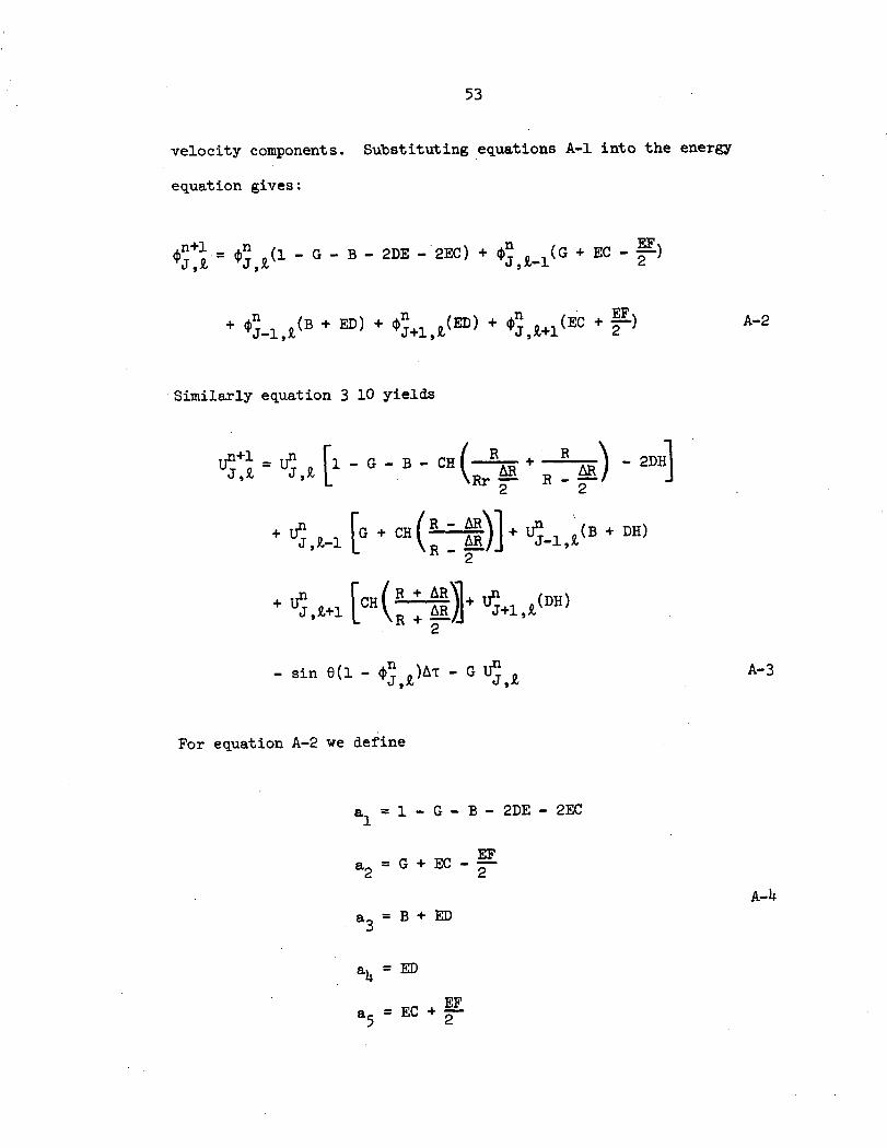
53
velocity components. Substituting equations A-1 into the energy
equation gives:
n+Jl n (1-G-B-2DE-EC)+- F.l= nz(1 - G - B - 2DE - 2EC) + on ,(G + EC - )
J,k i Jz-1 2
+ l i, (B + ED) + *Jn+1 (ED) + ,+1l(EC + 2E )
Similarly equation 3 10 yields
Un+1 = Uj [, 9, 9 R
- G- B- CH(RrR
2
+ R2
+ j [G + CH AR+ UJ 1n (B + DH)
UJ-l,t
U L QaR + UR+1 (DH)
- sin 6(1 - fjn )At - G UnJ~~k iJk
For equation A-2 we define
al =1 - G - B - 2DE - 2EC
EFa2 = G + EC 2-2 ~~~2
A-4
a3= B + ED
a4= ED
a5 =EC +2
A-2
- 2DH]
A-3
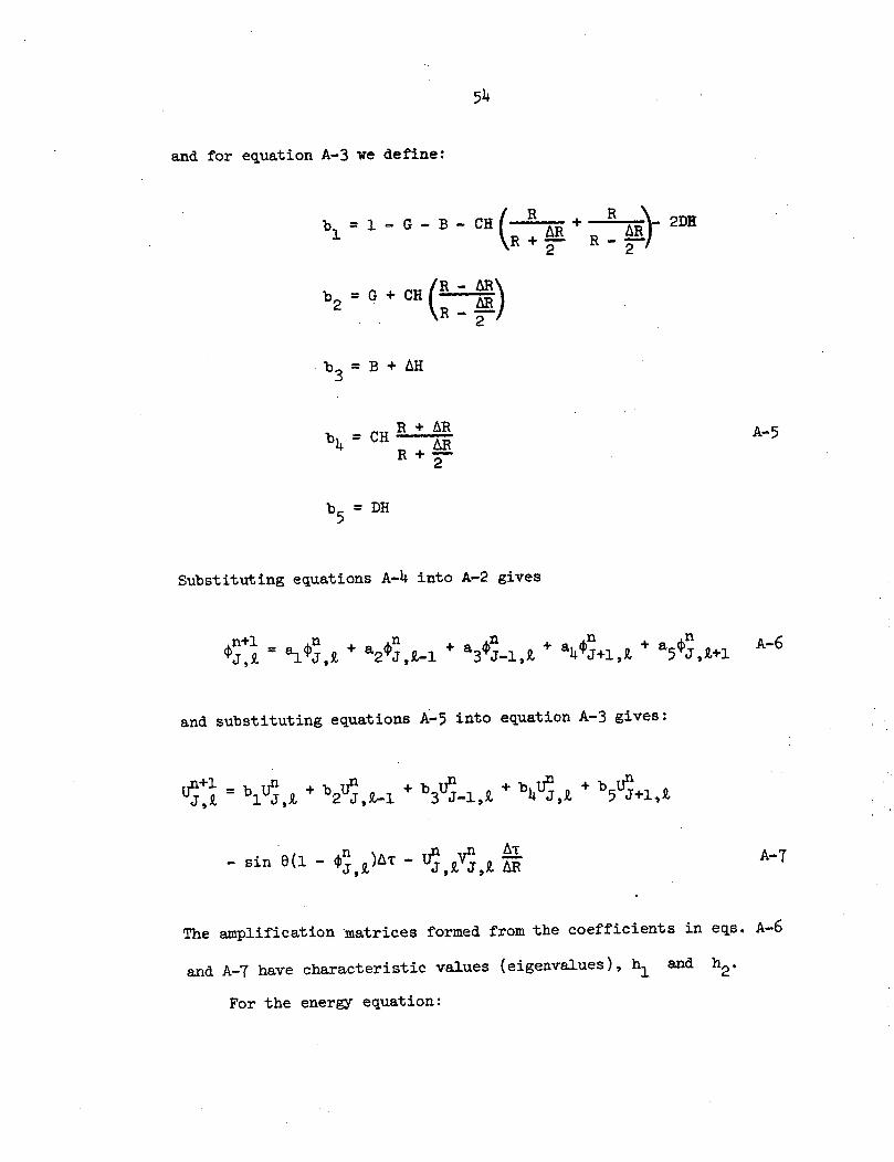
54
and for equation A-3 we define:
b1 = 1 - G - B - CH A( + R 2DI( 2 2R
b2 = G + CHR
-
b = B + AH
b~ CH R + ARR + AR
b5= DH
Substituting equations A-4 into A-2 gives
n+l n n n n nJ, = aljQ + a2 j Z-1 +a 3 J-1, + a4oj+l,, + a5 J,Q+1
and substituting equations A-5 into equation A-3 gives:
Un+l =blUn +bUQ + bUn lA b4 U, 5 J+1,J,- i JY 2 nJ,.- 3 J-1,k 4 + U J+1,
iJk iPJ,. J,£ AR
A-5
A-6
The amplification matrices formed from the coefficients in eqs. A-6
and A-7 have characteristic values (eigenvalues), hl and h2.
For the energy equation:
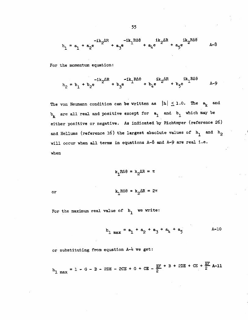
55
-ik2AR
hi = a1 + a2e
-ik RAe+ a3e
ik2AR+ age
ik2RAe+ a5e
For the momentum equation:
-ik2AR
h2 =1 + b2e
-ik RAE+ b3e
ik2 AR+ b4e
iklRAe
+ b5e
The von Neumann condition can be written as IhI < 1.0. The ak and
bk
are all real and positive except for al and b I which may be
either positive or negative. As indicated by Richtmyer (reference 26)
and Hellums (reference 16) the largest absolute values of hI
and h2
will occur when all terms in equations A-8 and A-9 are real i.e.
when
klRAB = k AR = T
or klRAE = k2AR = 2a
For the maximum real value of hI
we write:.1
hi max = a + a + a + a + a 5l max 12 2 3 4 5 A-10
or substituting from equation A-4 we get:
EFh = 1 - G - B - 2DE - 2CE + G + CE 2EF + B + 2DE + CE A-11
1 max 2
A-8
A-9
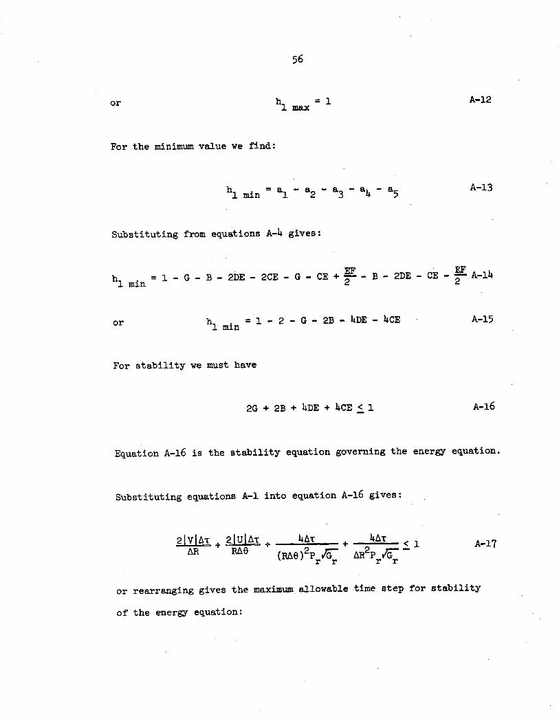
56
or h = 11hi max
For the minimum value we find:
h min al1 - a2 - a3 - a4 - a5
Substituting from equations A-4 gives:
EFhm = 1 - G - B - 2DE - 2CE - G - CE + 21 min2
- B - 2DE - CE - 2 A-14
h mi = 1 - 2 - G - 2B - 4DE - 4CE1 mmn A-15
For stability we must have
2G + 2B + 4DE + 4CE < 1 A-16
Equation A-16 is the stability equation governing the energy equation.
Substituting equations A-1 into equation A-16 gives:
2IVIAT + 2IUIA + A AR RAe (RAO)2 p vr'
r r
4AT
ARp r- -r r
or rearranging gives the maximum allowable time step for stability
of the energy equation:
A-12
A-13
or
A-17
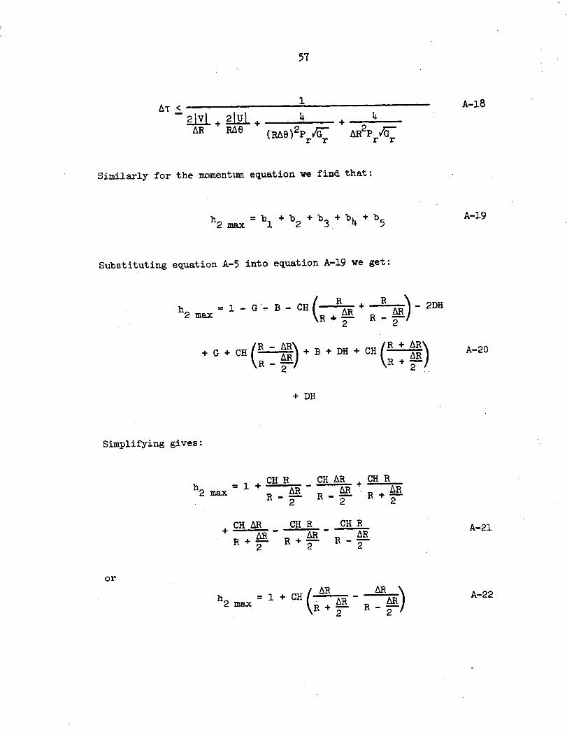
57
AT < 1
-21V 2I + 4 +AR RAe (RAe)2P vG AR2p vr
r r r r
Similarly for the momentum equation we find that:
h max bl + b2 + b3 + bq + b5
Substituting equation A-5 into equation A-19 we get:
2 max=1 - G -_B - CH R + R - 2DHA R-- 1 - G" B - CH(R 2 /AR+ -- - 2DH
R~ R
+ G + CH(R - R + B + DH +
2R -
CH(R + AR\
+ DH
Simplifying gives:
h CHA R CHAR CH Rh - 1 + R R2 max AR AR R + AR
R-- R-- R+-2 2 2
CH AR CH R CH RR + AR R R R+ R+ R-
2 2 2
or
2 m (CH AR R ARh2 max = 1+CHR AR
\R+F R-i--
A-18
A-19
A-20
A-21
A-22
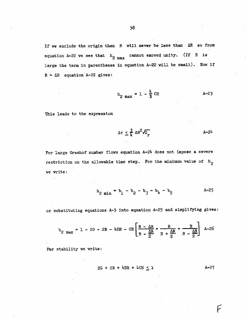
58
If we exclude the origin then R will never be less than AR so from
equation A-22 we see that h2 max cannot exceed unity. (If R is
large the term in parentheses in equation A-22 will be small). Now if
R = AR equation A-22 gives:
h 1--CH A-232 max 3
This leads to the expression
A T < AR2G- A-24A( < r
For large Grashof number flows equation A-24 does not impose a severe
restriction on the allowable time step. For the miniamum value of h2
we write:
h2 min = b - b2 b3 - b4 - b5 A-25
or substituting equations A-5 into equation A-25 and simplifying gives:
h2 = 1 - 2G - 2B - 4DH - CH [ hR R A-262 max we write:
2 R+
For stability we write:
2G + 2B + 4DH + 4CH < 1 A-27
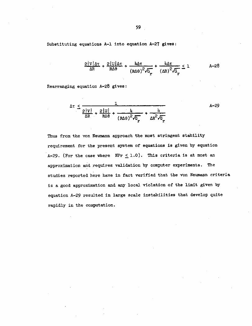
59
Substituting equations A-1 into equation A-27 gives:
2IIAT + 2UIAT + 4AT + < A-28AR RA 1 A-28AR RAe (RAe)2G (AR)e2
r r
Rearranging equation A-28 gives:
AT < - A-29-21Vl 21Ul + ,"m + + 2 + 4AR RAO (RAe)2 vG AR2 vG
r r
Thus from the von Neumann approach the most stringent stability
requirement for the present system of equations is given by equation
A-29. (For the case where NPr < 1.0). This criteria is at most an
approximation and requires validation by computer experiments. The
studies reported here have in fact verified that the von Neumann criteria
is a good approximation and any local violation of the limit given by
equation A-29 resulted in large scale instabilities that develop quite
rapidly in the computation.
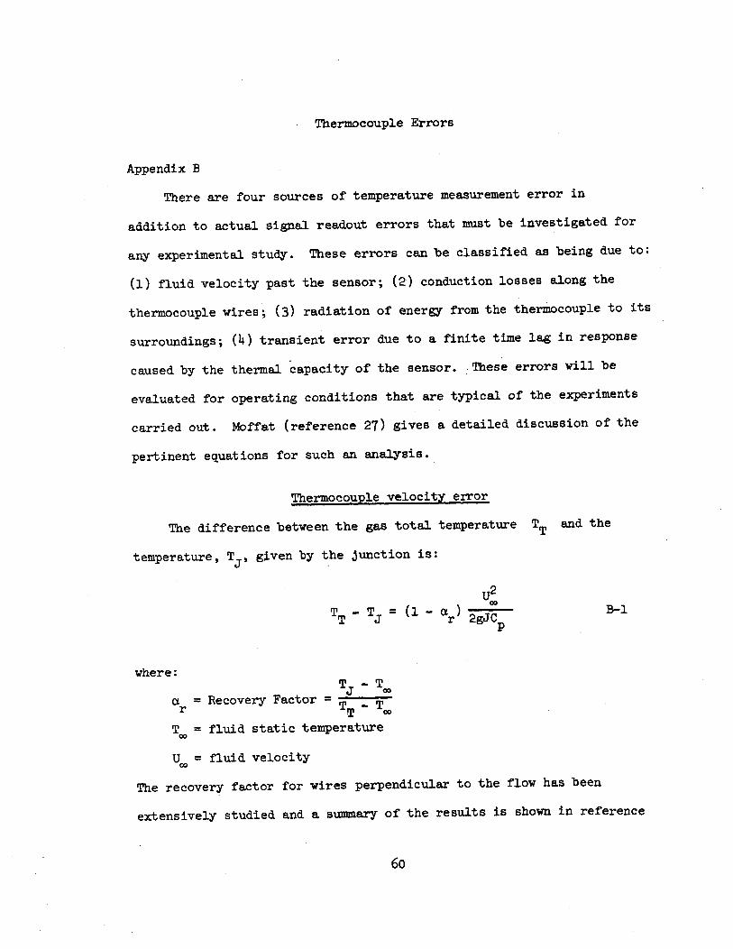
Thermocouple Errors
Appendix B
There are four sources of temperature measurement error in
addition to actual signal readout errors that must be investigated for
any experimental study. These errors can be classified as being due to:
(1) fluid velocity past the sensor; (2) conduction losses along the
thermocouple wires; (3) radiation of energy from the thermocouple to its
surroundings; (4) transient error due to a finite time lag in response
caused by the thermal capacity of the sensor. These errors will be
evaluated for operating conditions that are typical of the experiments
carried out. Moffat (reference 27) gives a detailed discussion of the
pertinent equations for such an analysis.
Thermocouple velocity error
The difference between the gas total temperature TT and the
temperature, Tj, given by the Junction is:
U2
TT T = (1 - r) 2gJCp
where:T - T
ar = Recovery Factor = T TT co
T = fluid static temperature
UQ = fluid velocity
The recovery factor for wires perpendicular to the flow has been
extensively studied and a summary of the results is shown in reference
60
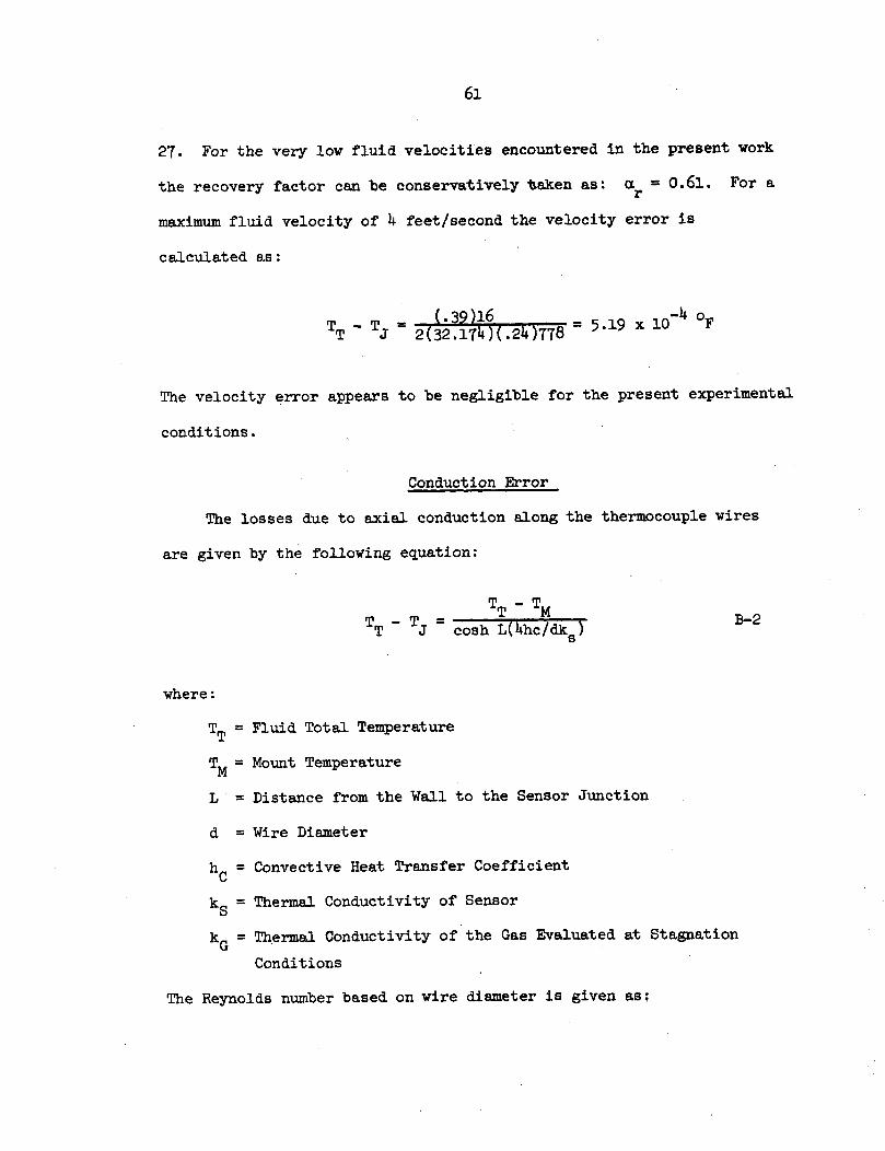
61
27. For the very low fluid velocities encountered in the present work
the recovery factor can be conservatively taken as: a = 0.61. For ar
maximum fluid velocity of 4 feet/second the velocity error is
calculated as:
T -T = (.39)16 5.19 x 10T J 2(32.174)(.2)7781
The velocity error appears to be negligible for the present experimental
conditions.
Conduction Error
The losses due to axial conduction along the thermocouple wires
are given by the following equation:
TT - TMTT - TJ = cosh L(4hc/dk s) B-2
where:
TT = Fluid Total Temperature
TM= Mount Temperature
L = Distance from the Wall to the Sensor Junction
d = Wire Diameter
hC= Convective Heat Transfer Coefficient
kS= Thermal Conductivity of Sensor
kG = Thermal Conductivity of the Gas Evaluated at Stagnation
Conditions
The Reynolds number based on wire diameter is given as;
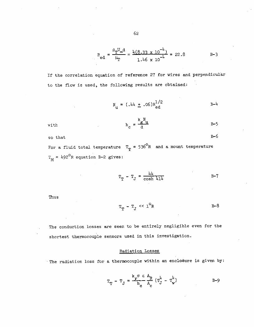
62
PTUod 4(8.33 x 10⁻⁴ ) 228
Red PT 1.46 x 10 -
B-3
If the correlation equation of reference 27 for wires and perpendicular
to the flow is used, the following results are obtained:
N = (.44 + .06)Rl/2 B-4u ed
k Nh = u
c d B-5
so that
For a fluid total temperature
TM = 4920 R equation B-2 gives:
B-6
TT = 5360 R and a mount temperature
T - T = h44T - TJ cosh 414 B-7
Thus
TT - TJ << 1°R B-8
The conduction losses are seen to be entirely negligible even for the
shortest thermocouple sensors used in this investigation.
Radiation Losses
-The radiation loss for a thermocouple within an enclosure is given by:
k a E AR 4 4TT -T rh A (T -T) B-9
c c
with

63
where
K = Radiation Form Factorr
a = Stefan Boltzman ConstantAAr = Ratio of Area Available for Radiative Loss to Area Availablec for Convective Loss.
c = Emissivity Compared to a Black body
For an enclosure that is large compared to the wire dimensions it is
known that K z 1.0.r A
For the present problem we may also write -Ar= 1.0. Also for oxidizedc
base metal thermocouples E - .85. And
Bt0 = 4.75 x 10⁻¹ 3 4 B-10
Ft sec R
Considering the largest gas to wall temperature difference to be 200 R
for the unsteady wall temperature decay of the present experiments,
equation B-8 gives:
TT'- TJ = 3.70 x 10 (1.14 x 10¹⁰
Thus (T -T)max 0. 420 R B-ll
Thus the radiative losses for the case of an unsteady wall temperature
decay can be of significance. Within the boundary layer there is
some reduction of the loss due to lower fluid temperatures. This
affect is partially overcome by a reduction in the value of h withinC
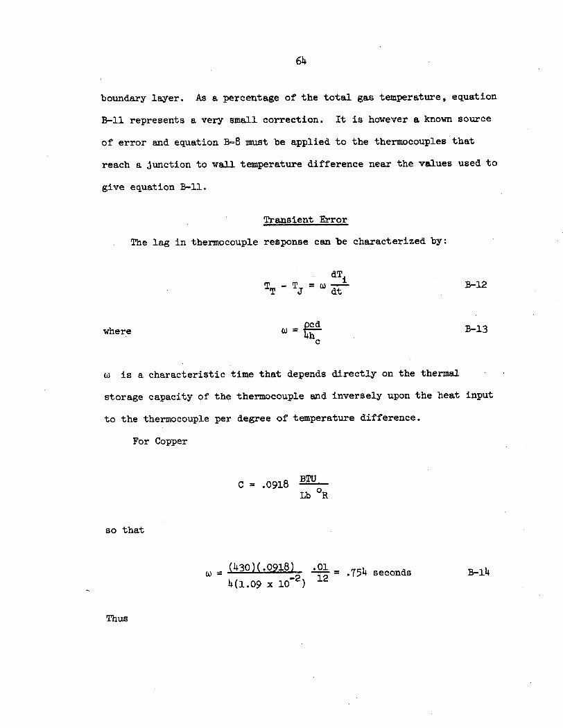
64
boundary layer. As a percentage of the total gas temperature, equation
B-ll represents a very small correction. It is however a known source
of error and equation B-8 must be applied to the thermocouples that
reach a Junction to wall temperature difference near the values used to
give equation B-ll.
Transient Error
The lag in thermocouple response can be characterized by:
dTiB-12TT - TJ = W dt
where B-13c
w is a characteristic time that depends directly on the thermal
storage capacity of the thermocouple and inversely upon the heat input
to the thermocouple per degree of temperature difference.
For Copper
C = .0918 BTULb OR
so that
= (430)(.0918) 01 = .754 seconds B-144(1.09 x 10 2 ) 12
Thus
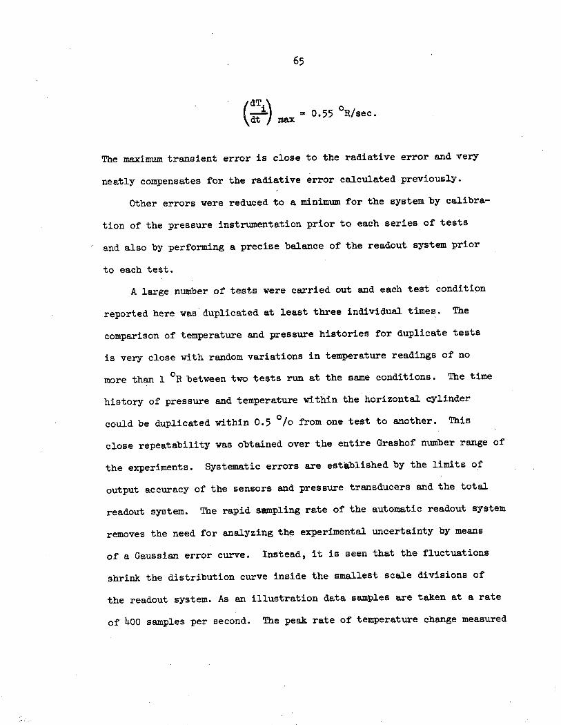
(I-) x = 0.55 OR/sec.
The maximum transient error is close to the radiative error and very
neatly compensates for the radiative error calculated previously.
Other errors were reduced to a minimum for the system by calibra-
tion of the pressure instrumentation prior to each series of tests
and also by performing a precise balance of the readout system prior
to each test.
A large number of tests were carried out and each test condition
reported here was duplicated at least three individual times. The
comparison of temperature and pressure histories for duplicate tests
is very close with random variations in temperature readings of no
more than 1 OR between two tests run at the same conditions. The time
history of pressure and temperature within the horizontal cylinder
could be duplicated within 0.5 0/o from one test to another. This
close repeatability was obtained over the entire Grashof number range of
the experiments. Systematic errors are established by the limits of
output accuracy of the sensors and pressure transducers and the total
readout system. The rapid sampling rate of the automatic readout system
removes the need for analyzing the experimental uncertainty by means
of a Gaussian error curve. Instead, it is seen that the fluctuations
shrink the distribution curve inside the smallest scale divisions of
the readout system. As an illustration data samples are taken at a rate
of 400 samples per second. The peak rate of temperature change measured
65
66
was close to 10 R per second so that effectively 100 sample readings
were taken within each 1/4 OR change in the value of temperature. For
machine plotted data this is about the limit of scale size that can
usefully be worked with. The data readings are truly scale limited
rather than being perturbation limited. The absolute uncertainty of
the temperature measurements is set by the error limits of the
thermocouple Junction itself. All known system errors are far below
the thermocouple error which commercially is given as + 1 1/20 F.
Calibrations of the thermocouples within a controlled ice point instru-
ment showed less than 1/2 OF discrepancy between recorded signal and
the ice point temperature. The temperature measurements have an overall
uncertainty of something on the order of + 1 l/20 F which is within about
+0.2 °/o of the measured values.
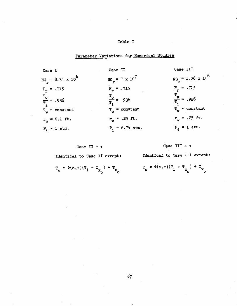
Table I
Parameter Variations for Numerical Studies
Case II
NG = 7 x 10⁷
r
P = .715r
w = 936
T = constant
rw = .25 ft.
Pi = 6.74 atm.
Case II - T
Identical to Case II except:
T= (o,T)(Ti
Tx ) + TO O
Case
NG =r
P =r
TW
Ti
T =
r =v
Pi
III
1.36 x 10⁶
.715
.936
constant
.25 ft.
1 atm.
Case III - T
Identical to Case III except:
T =c (o,T)(Ti Tx ) + TO O
67
Case
NG =r
P =rT
W
T.1
T =w
Pw
Pi
I
8.34 x 10⁴
.715
.936
constant
0.1 ft.
1 atm.
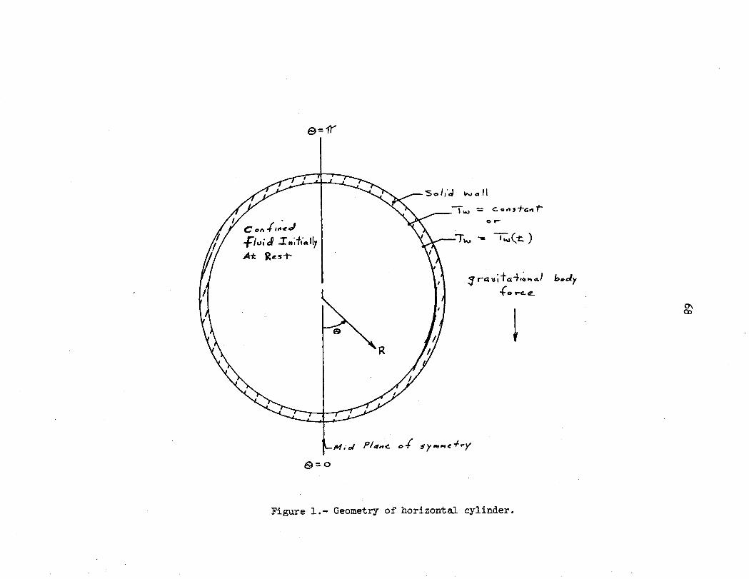
c 1,
o1 .--
L,
II P
L
68
IQ.0
IIQ
)
4)Hrdo0*,40 -4-ooq)
or.0I a4ii
0II
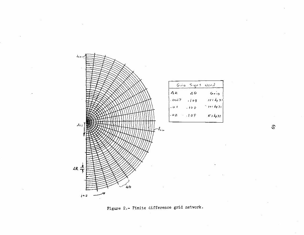
69
0r0go Ianc) aa)4-rd.H
IS'7
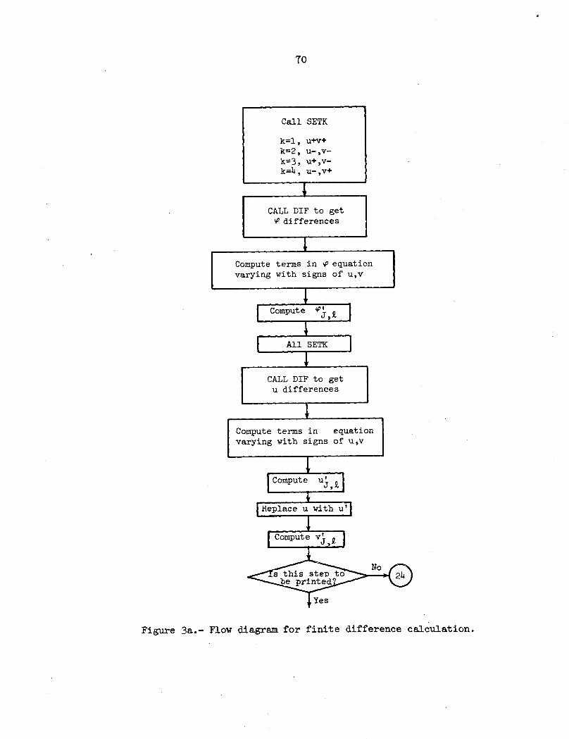
70
Figure 3a.- Flow diagram for finite difference calculation.
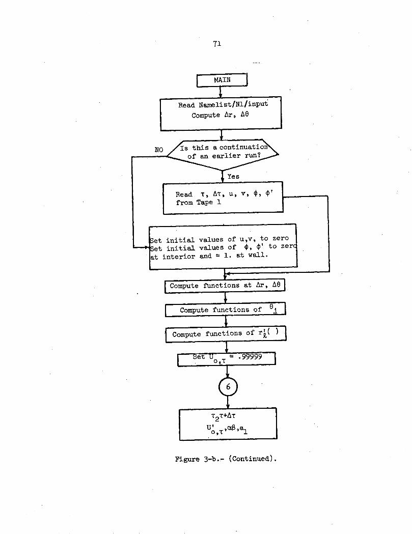
71
Read Namelist/Nl/input
Compute Ar, AO
Is this a continuati(of an earlier run?
Figure 3-b.- (Continued).
initial values of u,v, to zeroinitial values of *, *' to zerinterior and = 1. at wall.
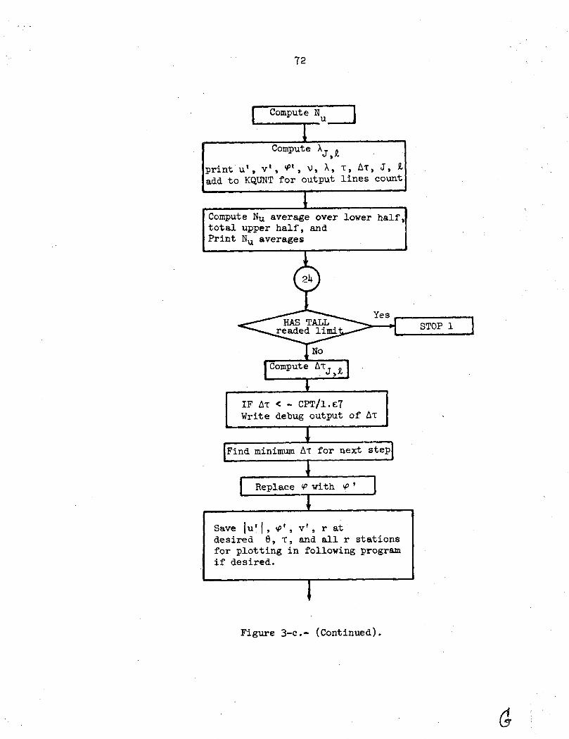
72
Compute Nu
Compute hJ
print u', v', ft, v, A, T, AT, J, iadd to KQUNT for output lines count
Compute Nu average over lower halftotal upper half, andPrint Nu averages
Yes
IF AT c - CPT/1.E7Write debug output of AT
Find minimum AT for next step
X _-I Replace P with 'P'
Jr
I
I
Figure 3-c.- (Continued).
4
Save (u'f, I', v', r atdesired e, T, and all r stationsfor plotting in following programif desired.
STOP 1 I
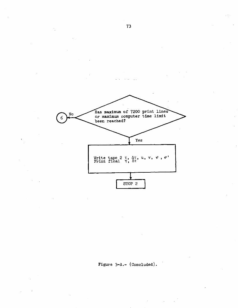
73
Has maximum of 7200 print lineEor maximum computer time limitbeen reached?
Figure 3-d.- (Concluded).
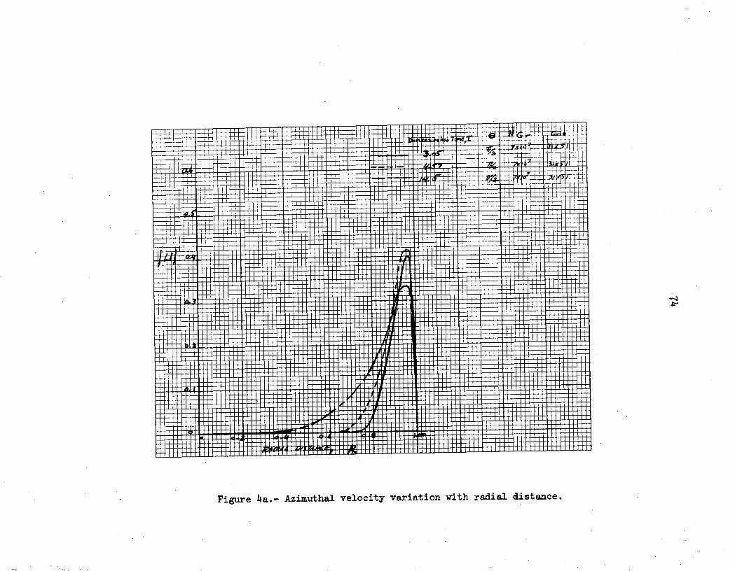
74
r400I +-a.1 4.0r
l
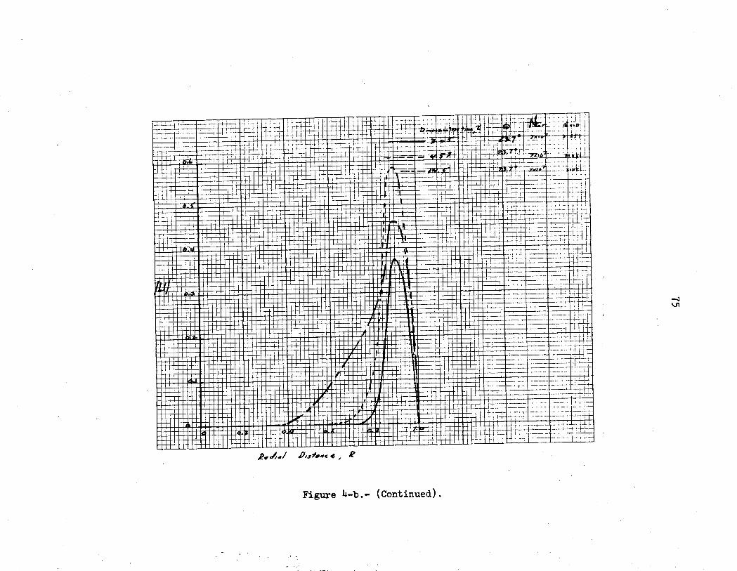
75
i' ii / t
I 1 !
--
I I
-.! i
--------
i~~i-: r 1 r1
: j Ij
i i i i~~T
TTT-
1t-tv-:P
ie
h-a-t-+
- t
-tI, _ i
.4 .
a0,4 0.r!F
4N
X4 l K* AX i t It 1 II , i I I
I
Ir.,4 i
,-i~ Ti-I
Xl, tl I ill
-li Xi-
--a T
1
_i
_'I
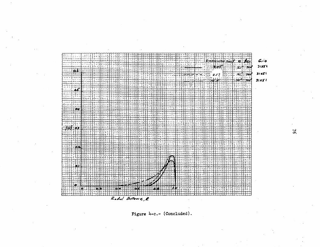
76
LL
iX
f i l.-
MW
040 g e | ; N
t4
t Ad X
X
t t X t 111 j1
||111f1
111g-1
1|tt1
Xt
X
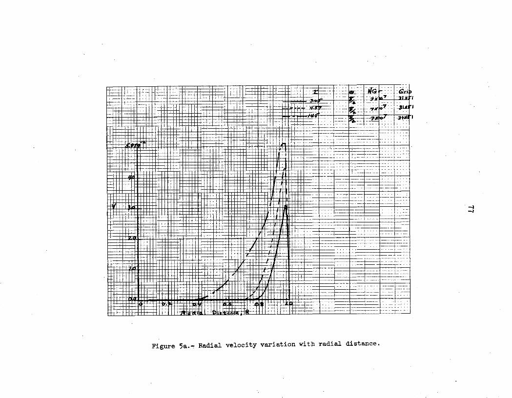
iB
I~~~~~~~~~~~~~~~~~~~~~~~~~~~TLI
......., ~
; ;:·
7 i i
·~~~~·I I~
,
; _I
..
wF
tI
t t
--i
--:'li
iii! !
l t
r.~;~
.i'~
~ i, !: i
i i
i I
!1
1i
,; ..... -j tT
t-t__ t
t, i1
1i
-_
4 -H
_
_ _'
i i
i ' i
i
H
X A
_ S
C_
_:St'iI _ll
i~ i.i'; i
ii ;t
i'..Ii
:~: II
,, ~-'
illR4!~A
-Fm
I
i~~~~~~~~~1 ~~~I
L
ll lliH
~I~~~~~~
~ ~
~~~~~~~~~~~~~~~~~ I
Illll'i
:~:
i il
i i~~
~~
~~
~~
~~
~~
~~
~~
~~
~~
~~
~~
~~
~~
~~
~~
~~
~~
~~
~~~~~~~~~~~~~~~~~~~~~~~~~~Ill
,,, -::i- ,4
fifilii:,
~~
~~
~iu
77
C,cI a,
.,-rda,I>4.r rl.ra 0V
I
ID
-*,
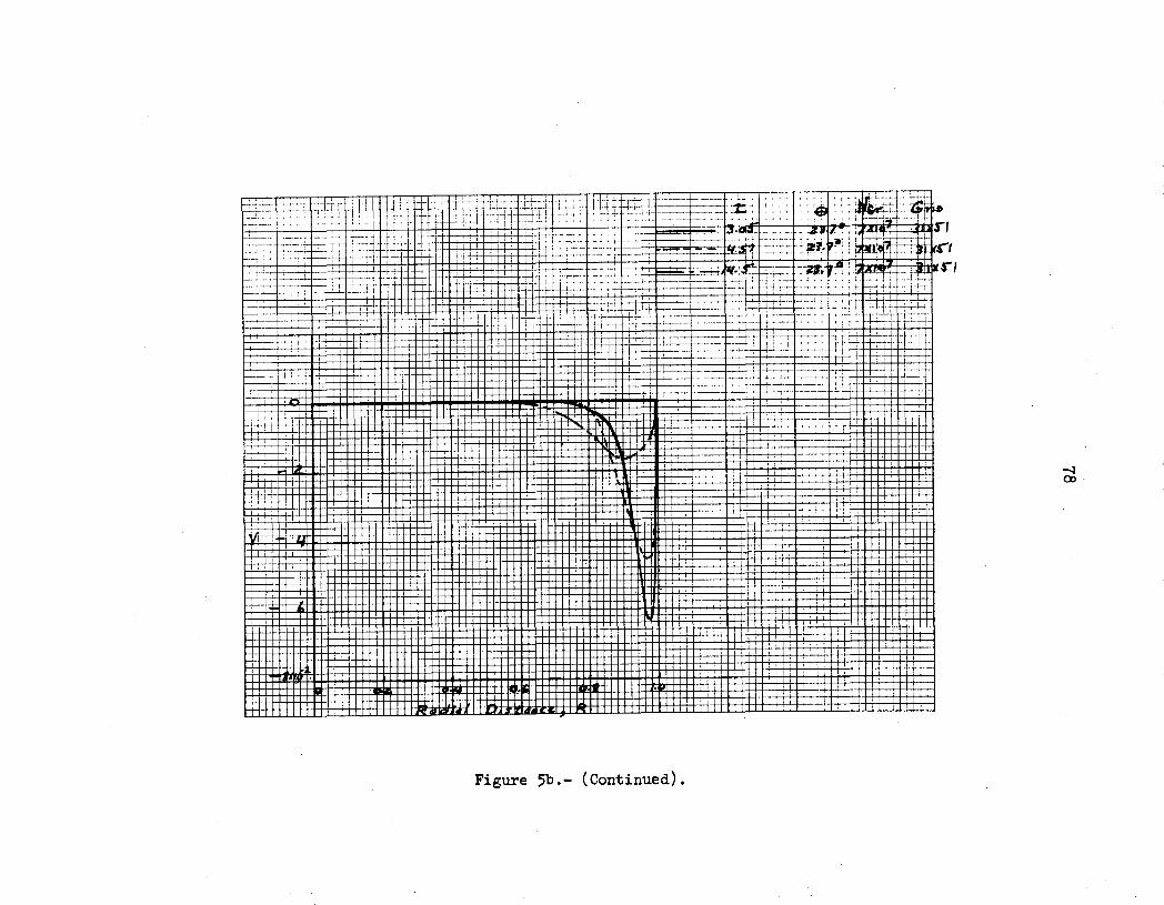
78
i. .II- ..
reb: ii lijil ;0
i ~
i+ '
i ~
L
:i
L~1ti1t
MI- ti
-111X
,0
l
ol! I
t t1
1 1 LI
IT-1
1 J" '
T~
~~
~~
~~
~~
~~
~~
~~
~~
It] .
' '
'~ ~ ~~~~~~~~II
I I
I I
I I· i
1.i it
i
~ ' I- ii,
1~
~illItiil
i~
I
rT-:
'I'' lll'1
I llt11111
I~I-RI1
'. ....
!1'
~ i~
I
I ~
tlli
: ~~~~~~~~~~~~~~~~~~~~~~~~~~I
"! ..
.';
I 1
Il
!- :---! ~''-
."::
_ ~
. ..
''""
,I
_11
Id4.,0vG)
.r, 1 4
I t_;
t:T
-I_!~
,dM_! -
--
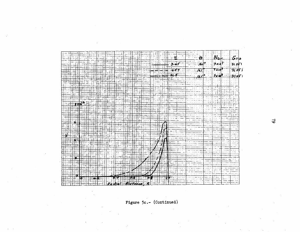
79
=C
L
4 C
CS
2
*t f
itt~~
~~
~~
~
i~~
~~
~~
~~
~~
~~
~~
~
~~~t '
i
Tj k +
i
_- 4
-T
-
ii j
I::n
:~~
~~
~-
Vf
I i
I i
t i
I I
' -
Ii LT I
LE .
M -1
-1T-
12
.,rza
i ri it-iti?-
�ffTF
I -9
r. K
-
.- WrTr
-i- t
4.L1L" -P-i-__F T
a _
I ,
_-
,1;.,
.iI
_
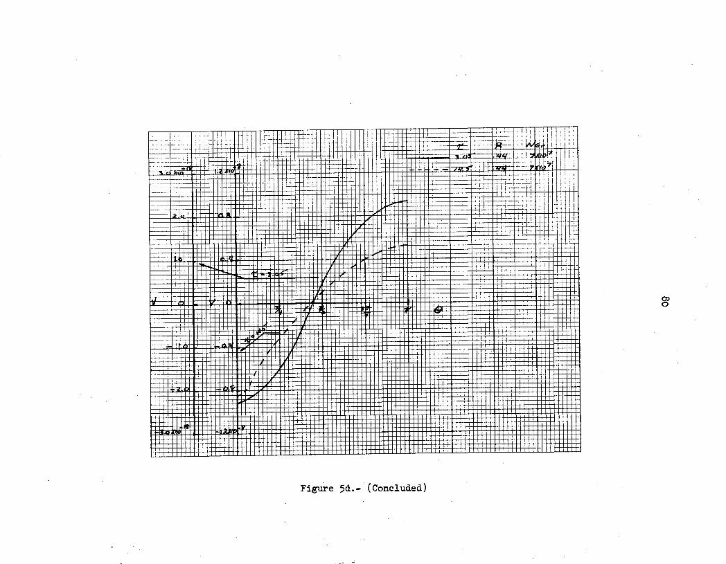
80
-- fK
_-_
-
IL-
-
or.0ua,4
· X
-- X-
t CT m; t I I I
iI f il IiI
-- t- -
i -'
~~~~~~- I t 14It!!
1-1
~~
~~
~~
~~
~~
~~
~~
~~
~~
~~
~R
-
m 4
4400t
<
i- -1
ff4
I: X
- 1A
·-~~
4-~
· ·
· :611
_- I, .f t*-'' f
. .1
, I
:. -fi I i
.I
I <
1
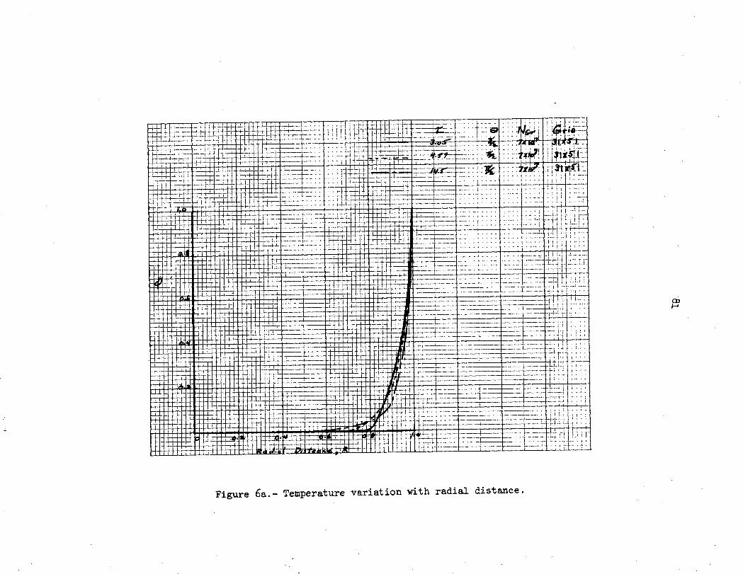
81
iTI
T -, .-
-, ri _
..T ' i i
+
W
i _,1
_ ,_
~~1 ;i~~
7
, #T
.~~
i
..
j i
l 0
0 t
i
,4. -1 4 -itl i
t :t4
U3U)
.,0·-1'Id4) HaIdCd
SdO ,14
4-)k 0.h .,ItPha IL,
E-e Cd
IL
\0 b4
4)
,tD4)
I
,t 4{
Ft -tX" A
~-" R
C
Si,, !11 t
I'll f
-i
'iT: 4
Ki~
i-. TI 7I_1
1 I L.
L I I
III
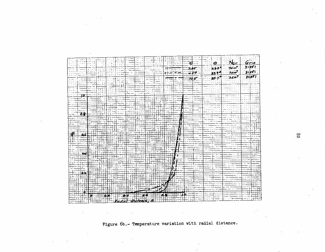
82
[f t X~~~~~~i:D~H
titT
_: '
1 r 1 i :
E
: : iti"
~ah ·
r h;:
r ·1
+
E
i :~~
~~
~Z
i
LII'A
14-~~~~~~
..
t X
iii L b
_ '! j t!+ i I j
ati
t S
a.,.J.,E4d
.IS0
!
ol$-(Dpq
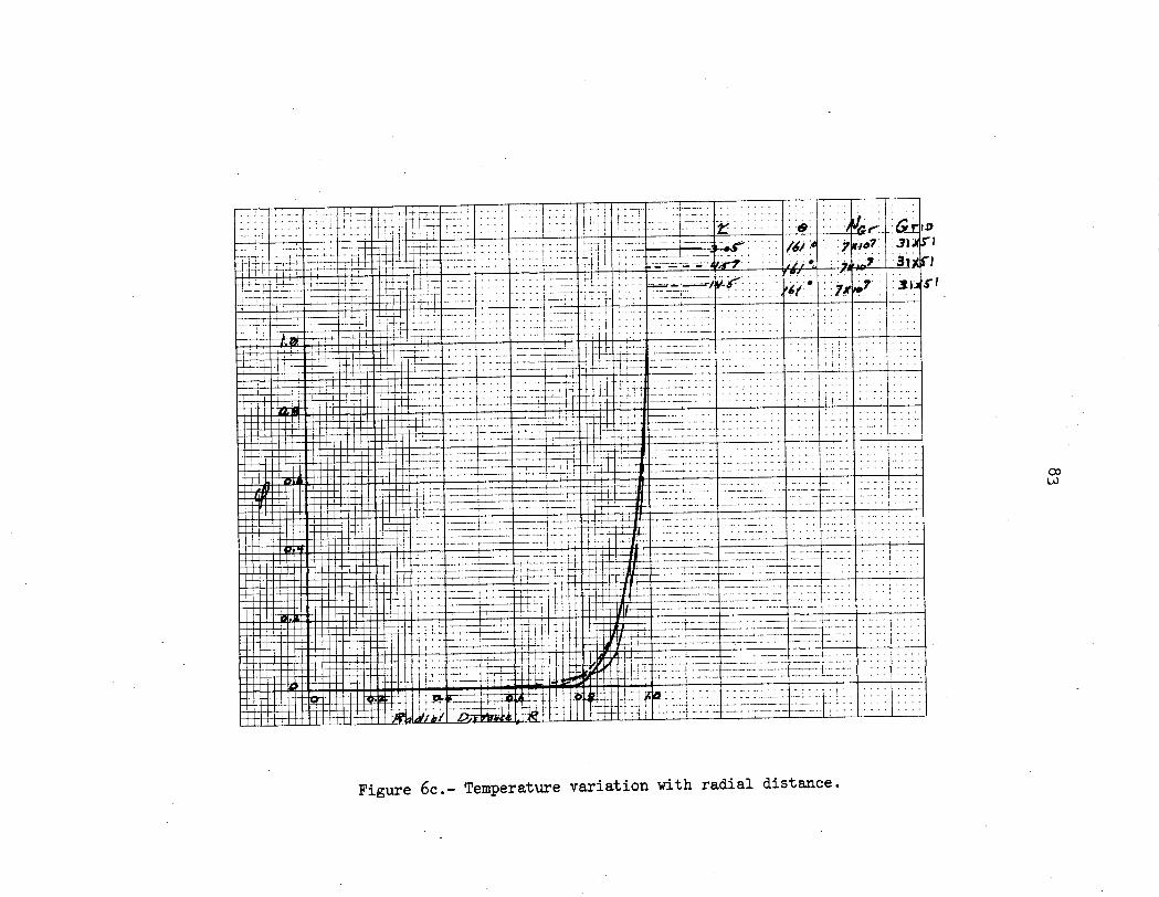
83
94; i;
_-
.q
{q ' '.
' '
' '
' 1.
', '''
., .
..' ....'.'
....
~~
~~
~.
..
..
..
..
...
.. .
... .
_._. .
_X_.._
-.
4 '
_ ~
~.
_''. .
., '-_ _
.1 ...,. .,.,;.i'...*_'
0 7i\ _, ,' .. '. '
i t i
::: ~::: ::: :::: :::i: :::: ::;: :i:.
!! 1l, iil
.;::I::1:: it 'a
l,-~
~
~4
--
·-·i--I -
· I ·
I 1
H
t~~
t7
f 1
i^
i 3
iI
i, l I
'K I
*I '1
' l.'T
.
Is· .
i iJ ' 1 .,
: I 1. ItIt.
PtPi- i
-HI
"- ,
;_ i -I
-I ;'
t C
ITi IX
tfl,,,,1
LX
r'riId.¢;:0 ',r\-
__. 2
-ItilI
' ;T T
-.....
- 1 . .h
-t-d t-
--. D
'IfI i i. : i Id
..-
., i-.
L. ' : ' ,i
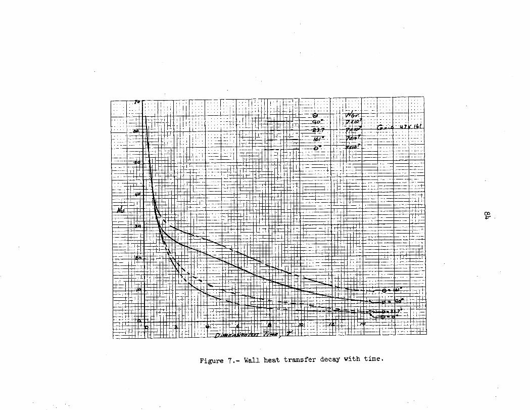
84
:it :;: X
t~ X
I Ii
'~~
~~
~~
~~
~~
~~
~~
~~
~
zXWj l U X
W;i
-T W
i W
T
X
r [ $ f t t X t t 0
iiii
nii~nIi 1i ~
i·+i
:-. i I ~
~ ~
~ -
++
+
-H44
i~ ~~
~~
~~
~~
~~
~l
4
4 II
I I
i r~~~~~~~~~~~~~~~~~~~~~~~~p
I t
0'H.,a,Ce
0)
'C I-ItaH
V14.rX
k
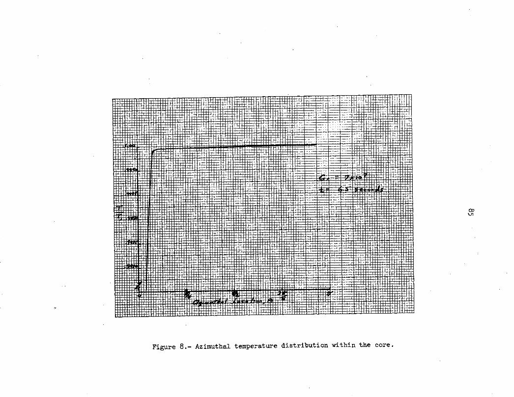
85
0o *4.4
4.) ., Nta)
+,^
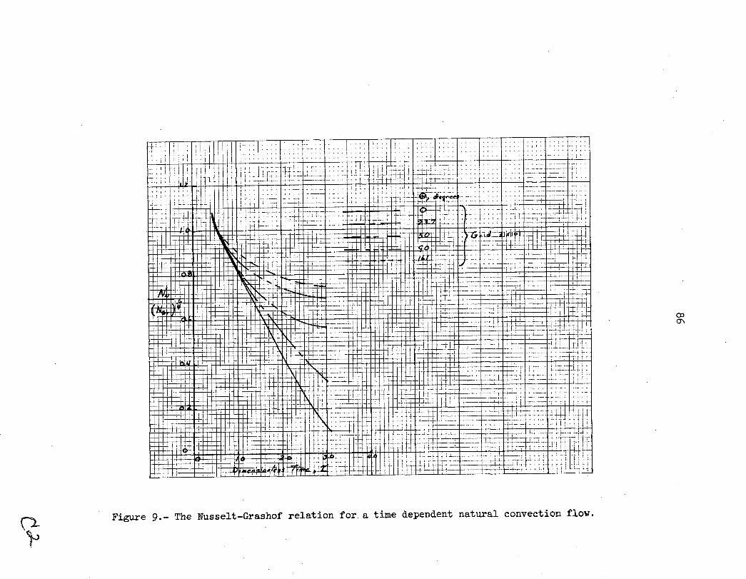
86
___ T
ft~
~~
~~
~~
~~
~~
~~
~~
-r
it
4j~~
~j
~~~{ Vj!. -
-111.9 jj ~~~~~~~~~~~ r4¼ 4
- 4-
I I
-17 -4
-1
-- ---
··TT
*----
I' -: -I
r{
I it=
L -
4 ~ ~ I-
i---: I-.-
li
T
I I
Ii I
i
1 4L
I II
i~I 44
~~~"' ~
~ I
4I-4
4-
-TI
··· t
I '----~
-~'-4
I1
-t- L-i
-,
1'. 4
-; -
.-I
:: T 4 , '
1 -4: 4
4 i
I j
+L
ETt -j
0oH00C
)
H .4+) uw0 Cd
es90)a)
r 0wa,'.4 00 0.'4, a,
.d0) '40U)
rqa, I'.4 04,
*H 00) U9
0)
1z10, I0, rn;j;40\
.,I
i-ti IH:
:
__
-.__
._ .._
1
' '
..
I ..
I I
_..I
_ 1. .
_ .'... --
L·
! -I-- -1 I
~.1
Ej
icffl Xt1EIrrt-F
Zr .-
H-! '
r-r-
n~~P~
;
;[:"i -i
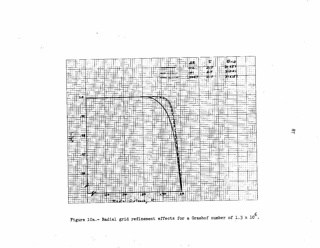
··· -- i I :-·-· · ·-· -·-·-· -··- -t
-- '-- .
..
..
..i.
.H
g .0 g0E LI..
i1%_
U4- W
-
t; :2 0 Wi
.iI F
44
.I i =
'4 ,_-
~~
~'<
""I:
"
+t
k1-1 Jtj
Ri1
0H0rj ci.oar0 C).r4 taDaS
, :4
87
i. I
r
7>
1 7 I
r! iI
F, r-7
T T-11 +- f- 1
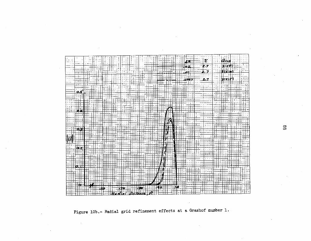
.L
.- A
:ti· . .
::- -.
: l
.- I.S..:
...'
.. ,
_ i. .
I ;
i~I
-I-
1H0C: 40a-
C,
V XX
~--L4-$ ~-I :-
_ I I ,,
il I _ i i
i.4 i
I I T-
1- -i-ii 1
i i
i I
88
4,Vwq4)
+)
.ardIo,rltA
I. .t I i.
,-... X
i ..
..' i
__ ii
___
_r
~:
I .I
=._ AL ..
..
.I
....-.1.!,Ii .1
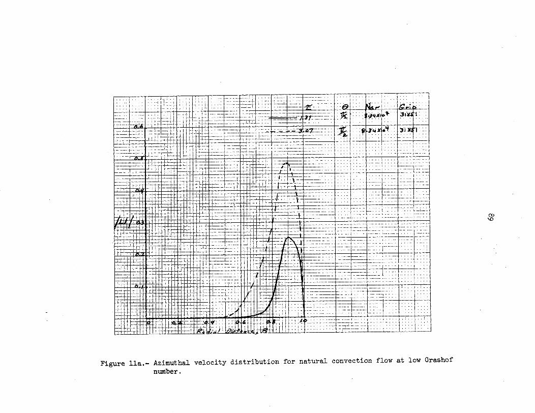
89
0
L.
.. ':
..,K
L
o ,
:":n
~~
h
X
,:0 i
:4
I-J
~ i j
::l ~i !i I i 11~11 1t{~~ ':ii i I I I i i i Iii I~~~~~~~~-in
ii I i i iii i i i
:I~
' I~
~
: ~~i ~~~i
~~i; 41
_+
___
H
H
-T_
1 --
:- I
J?
----
--
· -
-~--.
:!: ;i !:
j t~
:[' ' -
~-i
i ii i
Il-i
Imi-
cl i
I I liri
i-I -I I-i-~
ili·;·iJ~i~
--lh;L
~i~
-l .
H
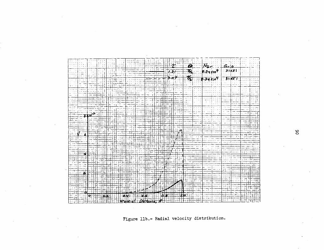
90
0oi0 -,q
.H0,-i
*,.rI--I
.rjr-4
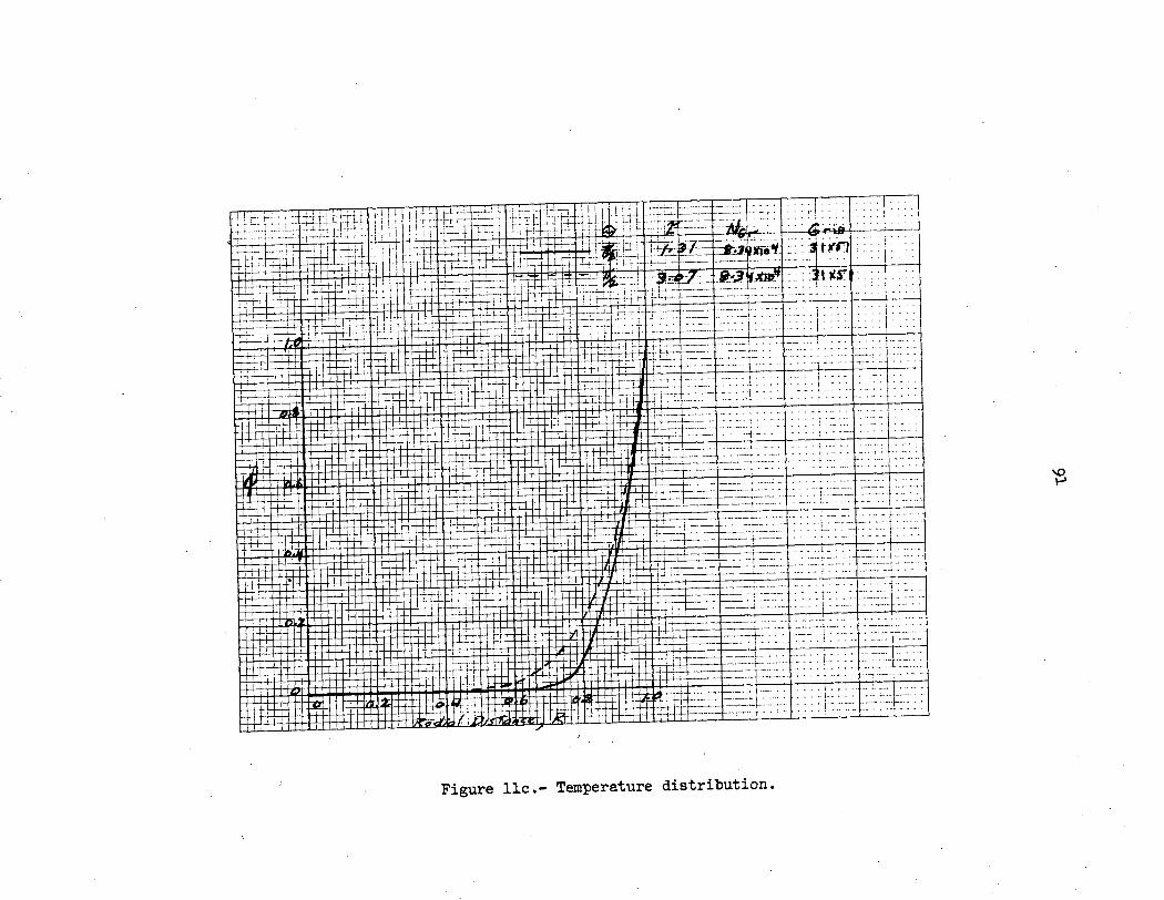
91
04o,-I
*rl*rlIA
r-4rTp4f,4
l
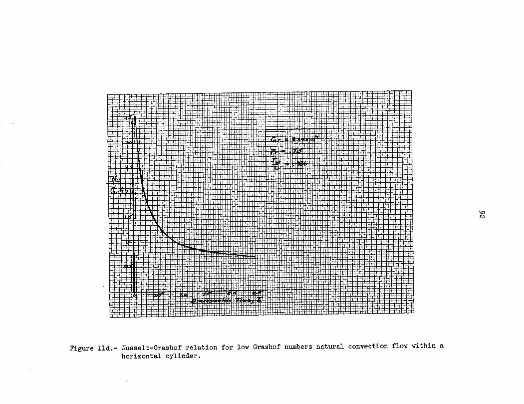
92
-r 4,0C
)
H.r'lo 0k C)
a)0C-)Ah o
4,-
0is.-
(0 -I
,t0
rd
hO
H
I
r-4
ci
*,1-
0
4.DI
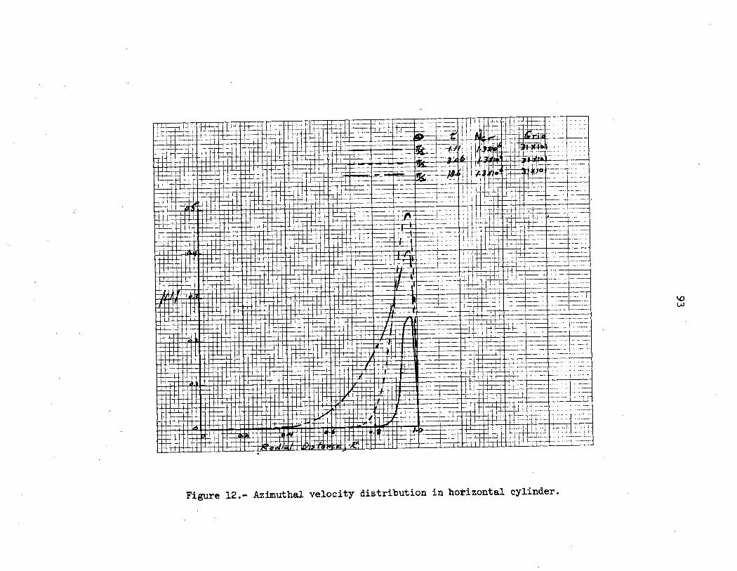
.1 T.
I _..
_ __
i W f S f V
f i
W
W F s
-v
_ i _ _
_ i
1 >
_ _
k
93
C,
400 *rl
or Ho>1 uIr-00 tqH44H0) 0I:
laI'
k -.,I00INA
4!oi
.rq1
FX
Cki
ii~fL
CT
t
l-tt-:
e t.1 1-1H
I; kIIIII
FMI-Td
iHT
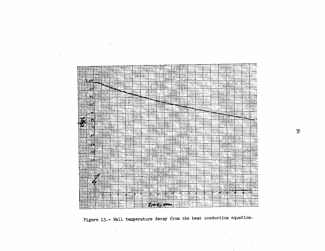
94
At-i tI ff-t t-ti{tH It] H
TH'th'Bi H
til thi
.| iI
t |
i 1:";
l
041o0c)0 0c9r-4I.,p
400r4
B X
S1iS
tF~
i i
N-44-:ft f f
tA~~~~~~~~~~~~~~~~~~~~~~~~~ : H
I I
II<
t I 1, I
g X0T
I X
X
X
X X
X
Q
M~~~~tittt
I I
MN
-1 X
II 11 1H
11111 112 ~ Hilil I
g g 1}-0001T-}-0,}--t0X~4H,1-111-1--0X
I g-X
I ~~~~~~-H ~
~ Y
44++-t
R Htj-10tqiu
I -:-!P :1.d
l-f7H-H
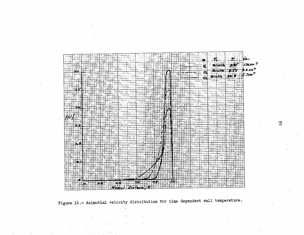
95
I',,.q
ai.4+)0)
od0)
4)I4) 4)
Hq
$4
rdW)
.r*,
tt
.. ,
X44+0 b--:
f Iljj
ii~
~ ~
~ 11I~
.4I...........i ,
HH i~~~~~~~II
L
r~~
~~
~~
~~
~7
:!
:-
iu 1 i
Il t t i ......
i!~
~~
~~
~~
~~
_x_
, >
IF
!I' ~
i !!~ l !! ! !!
!!!II
l~.~
Ilj l~klll
LIT :i Il:.q
IIIIII, , ,
, , ,
JJ'~
~~
~~
~
3
i-t-1, -i -F rfl tr It
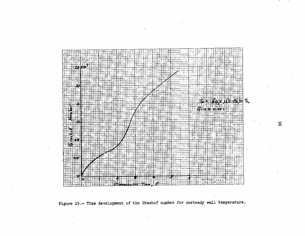
96
a)tqa k00)o 4)
UE I $4toa f4I,2UN
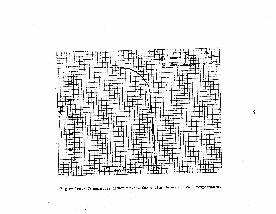
97
t P40a)
.,rl ,4 a)at 00atp4a)
E1-
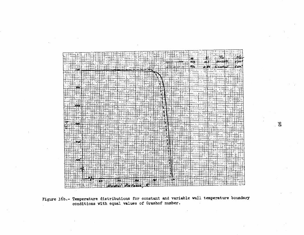
98
§0 op.,4-,0 a
a3 U,
4oH 0
3 sq
a o
oo
1o
k
I g
ka
4Sink:
0
oa d
o,1-4
PaJ
0h
4o
in-40
'
kG)
*., inrt
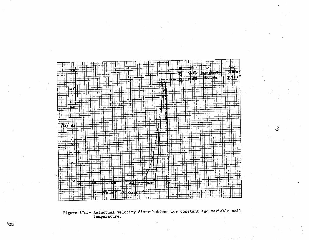
99
Hr-o.4,
Id 00S
cIon
4-5.-I wa.,ia
,.
>a)
rz
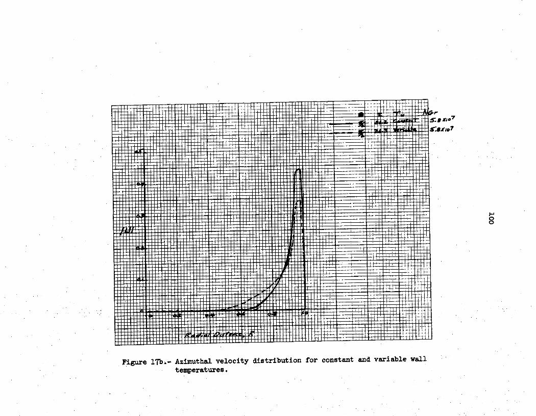
100
la4)0Co .4toN)
¢ 9rl
I
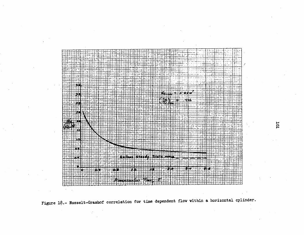
101
HU 0.9-$4
.ed
0'Cco
0 -ts4,4)4l0o0a.03
N
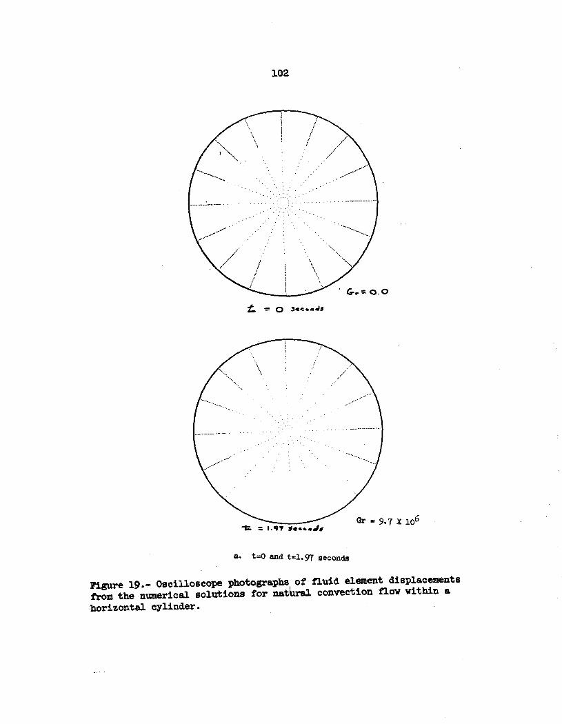
102
t -= 0 ~3(:." J*
Gr = 9.7 X 10⁶
a. t=O and t=1.97 seconds
Figure 19.- Oscilloscope photographs of fluid element displacementsfrom the numerical solutions for natr-al convection flow within ahorizontal cylinder.
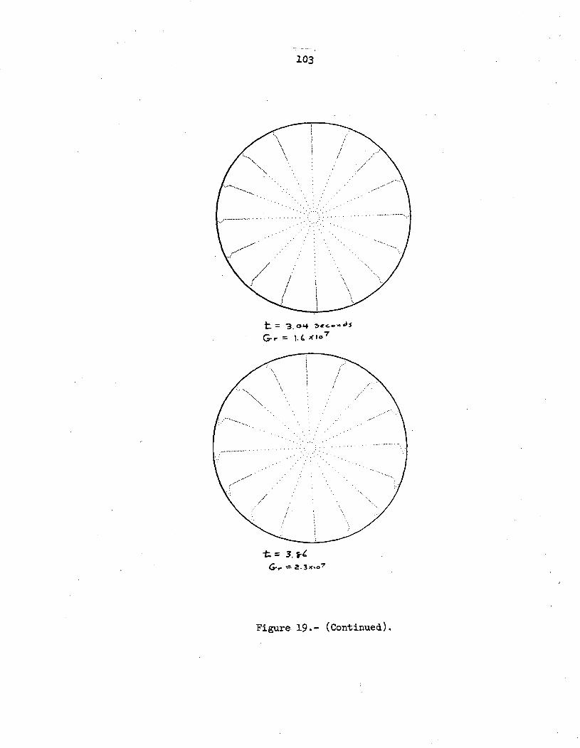
103
............ ......
" .. .:.. ..... ..
t= 3.o) a4o, J
G, = I.( x I °7
X= 3. o
Figure 19.- (Continued).
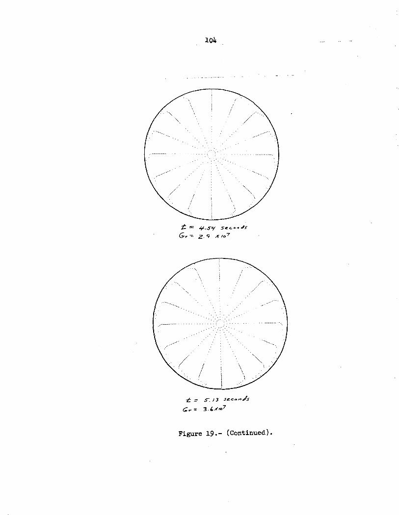
104
G.-r z2 Ao 7
6r = 3 . x ,o 7
Figure 19.- (Continued).
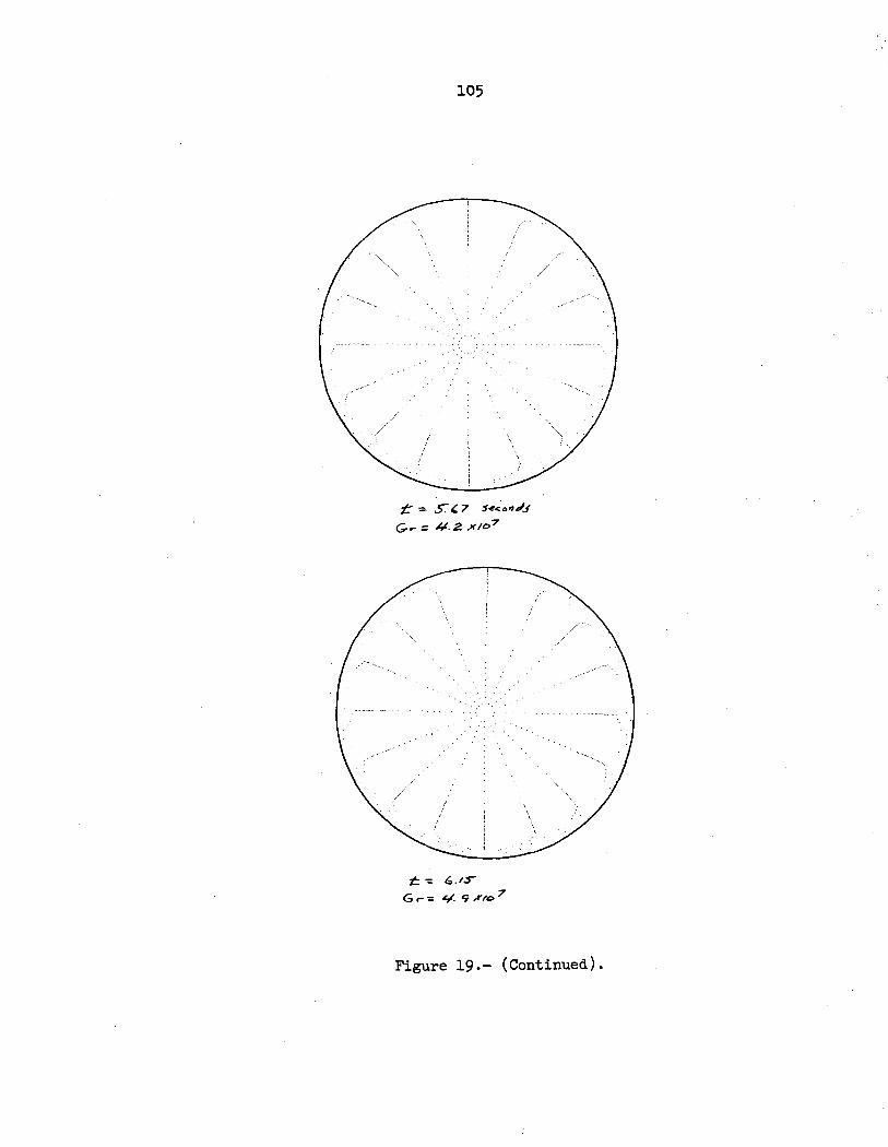
105
= - C 7 secod.s.
&r = 4. 2 X/o 7
G- = 6. /o 7
GC= 4/. 9 r/ 7
Figure 19.- (Continued).
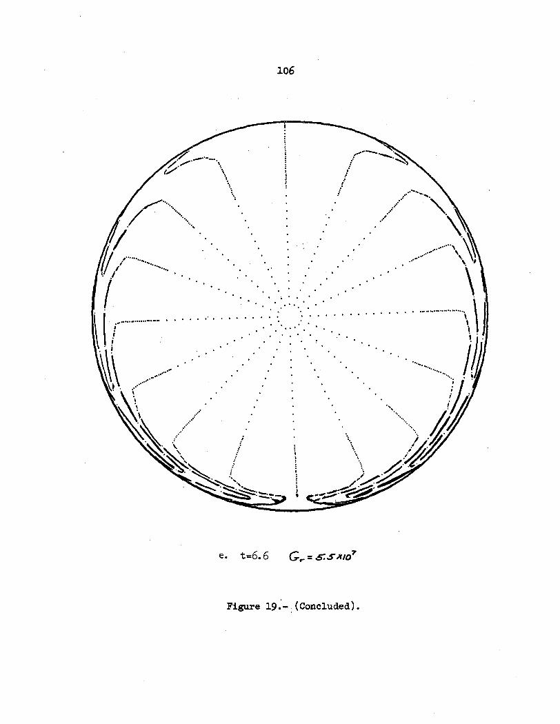
106
e. t=6.6 C. = SSSo
Figure 19.- (Concluded).
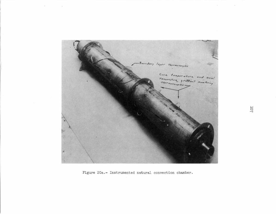
5 -J
Figure 20a.- Instrumented natural convection chamber.

4 ,H
CD
a
C
C..
4$4
to +
m
· A
"' I
4-'
108
cn
'341 a30W
i
.,3 OoI0.-4 Q,
,00r.
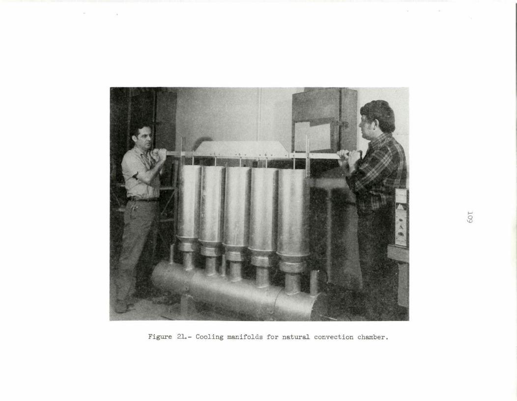
8
Figure 21.- Cooling manifolds for natural convection chamber.
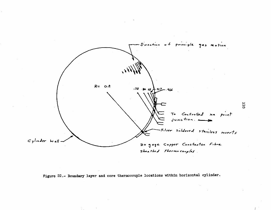
110
-k-C
Is~~~~ t
~I,r o
.0 "4:
' '
k z
c zr4
0 0~
.o
%4.
.4 oS
~. 4
L
Lh0
0)
6 0
-i
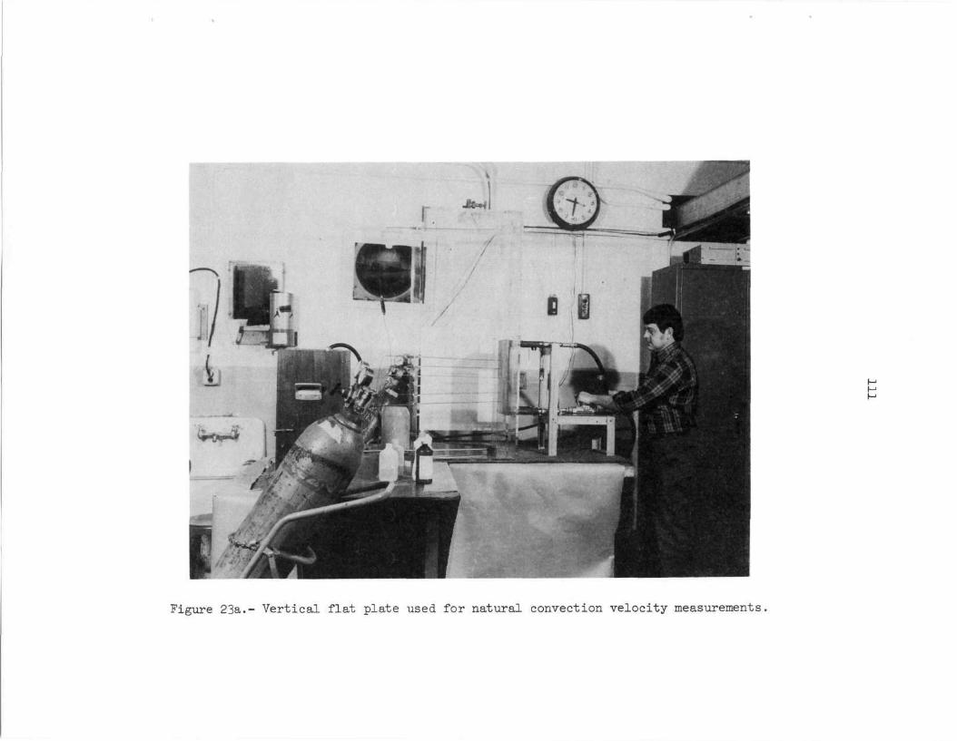
Figure 23a.- Vertical flat plate used for natural convection velocity measurements,
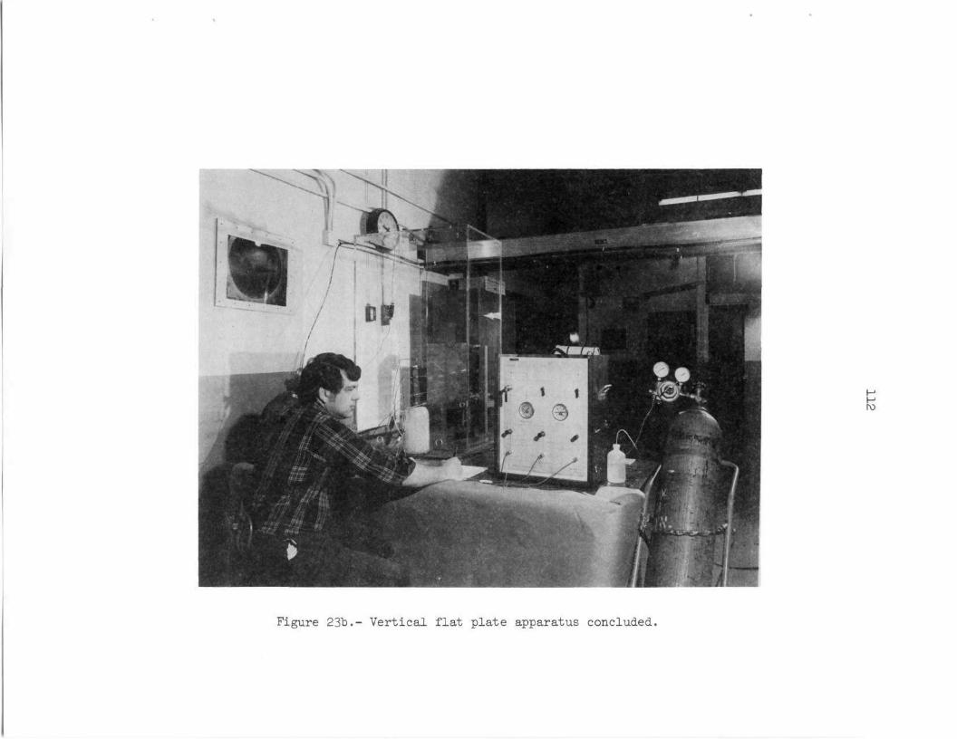
Figure 23b.- Vertical flat plate apparatus concluded.
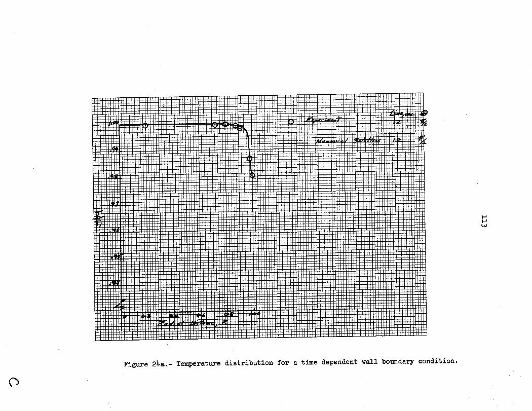
113
0.r44).r40V
.00t4 C
c
rd0ar.a)0s-I 04,
4) -0 oe I005.44)
h 41') LO
0E-405.4
·rx 0ICc
Q)
kr
.,
C
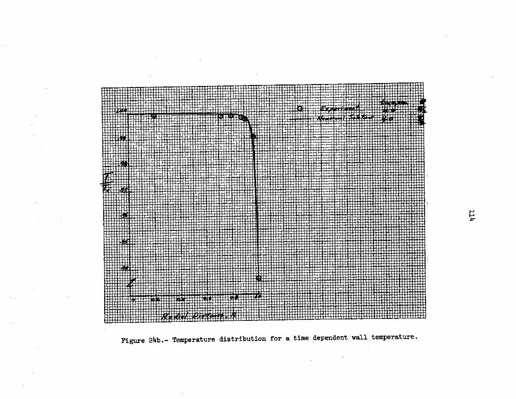
114
aN0U,
14a,
0pdSz 04dp..,1 04 '004,0 $4 00'a k 1.402
'01.H4, $4
0ptScu0 E-4
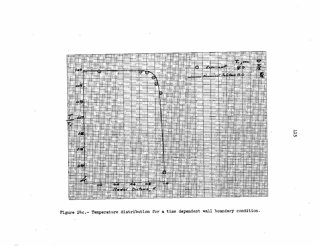
115
04- o.,o Ido ri:0 4, aPd
ao-r4
.:4 CU O
0.10
4ba,a)aa,.rxFr4
II
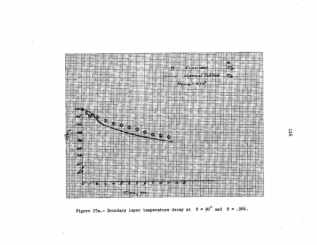
116
I'DoofoI 00oC)
0c
oo aI04,
rlI*,4N
r
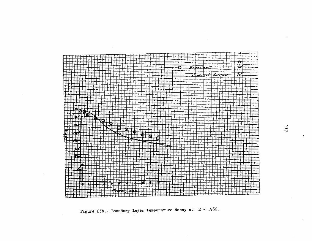
117
"DC,
4)4,
*4
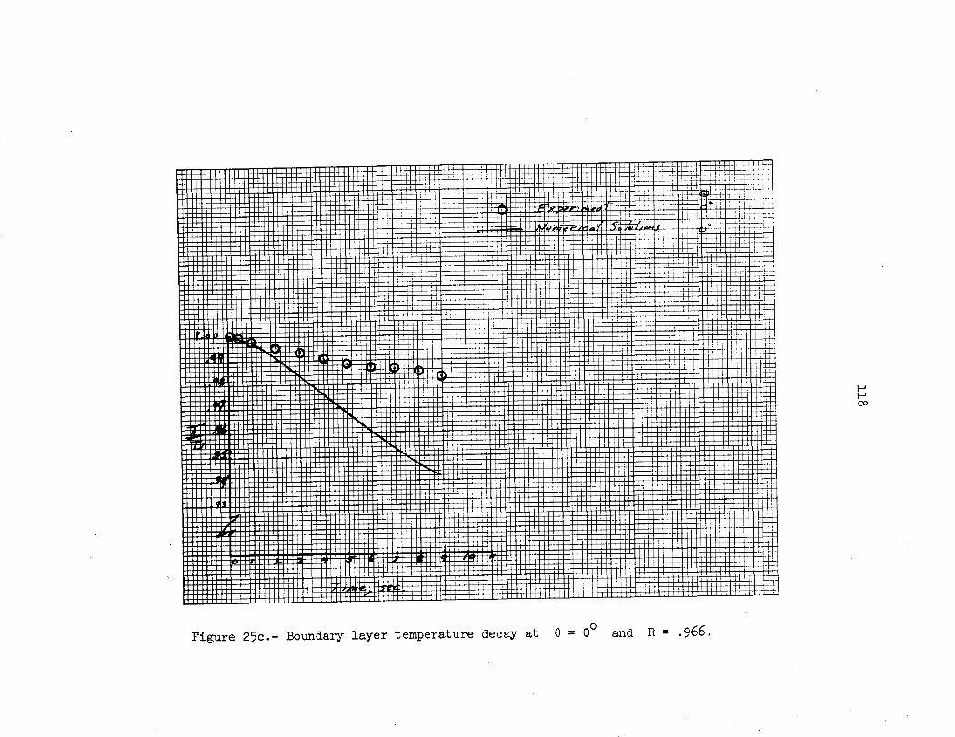
118
II
o1o
oCo
0II
CDIdC)
a)a) -q0) a,
'5
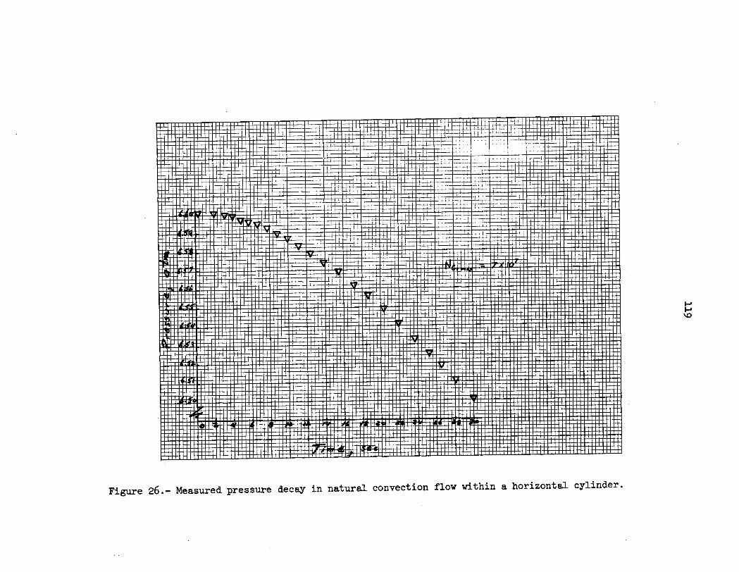
119
40rl00.roH0C)
o -,-0 CH
0.,p400ci
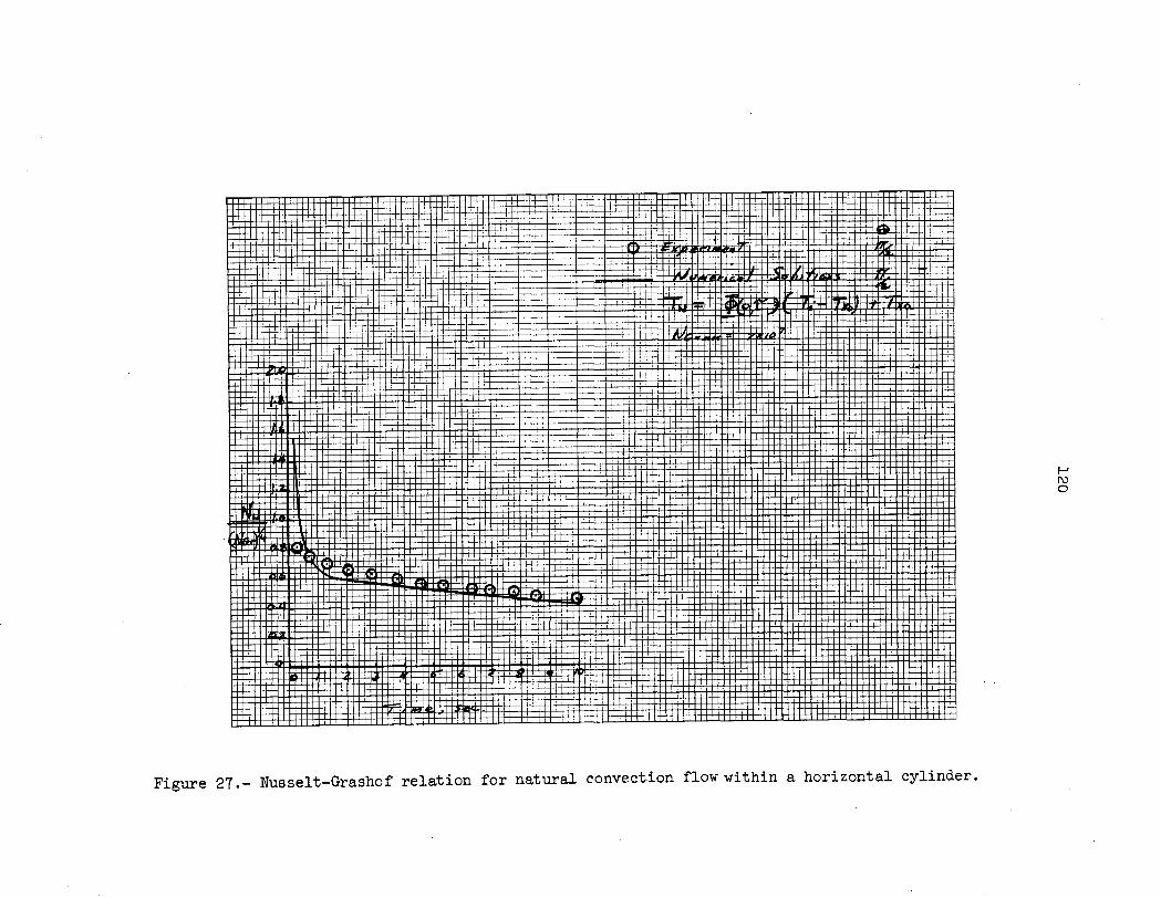
120
o '4C)
o0o.r-o 4-,
C.)
0 C"00 0C-
0O-Hr-4 4-t1)'-4
Ia
H
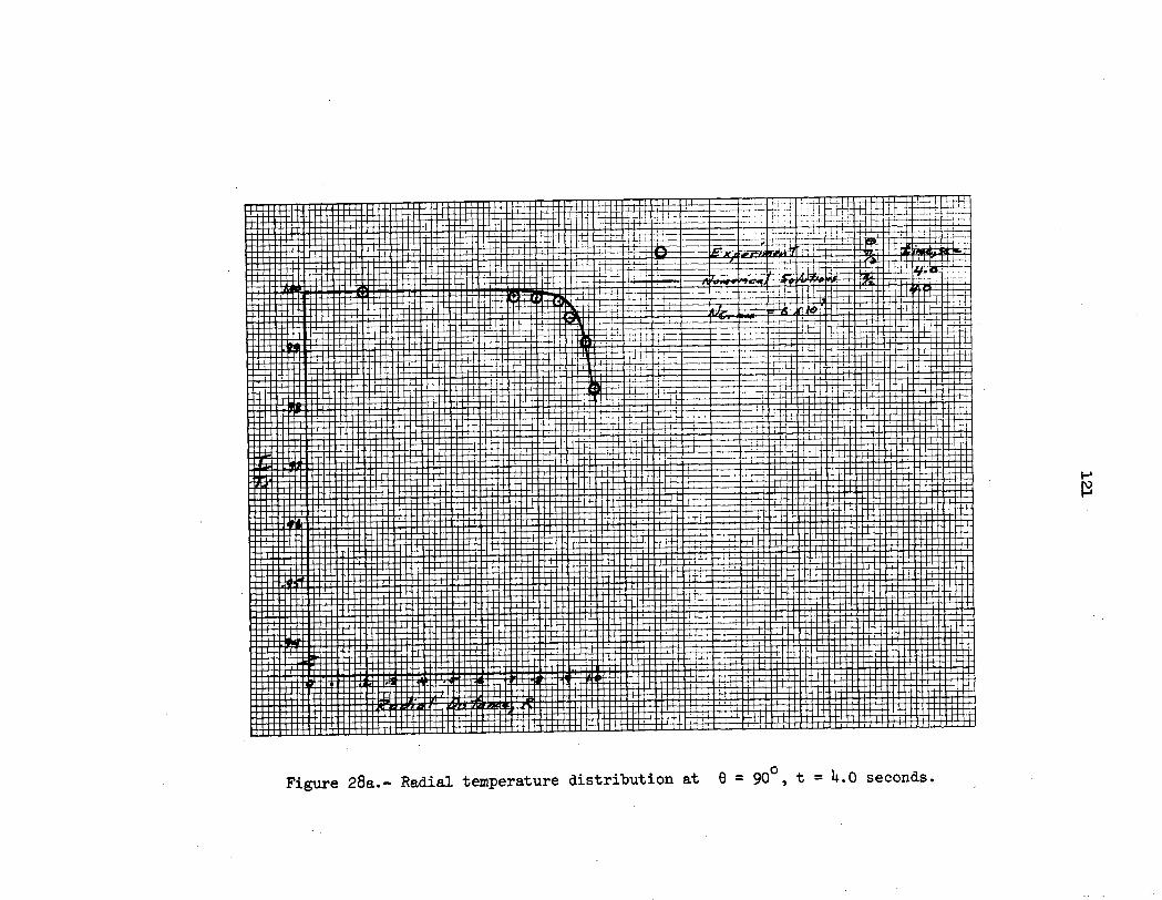
121
o c}o0.,II
4.)oco4.,r04,0p
I
.,fco0C
M
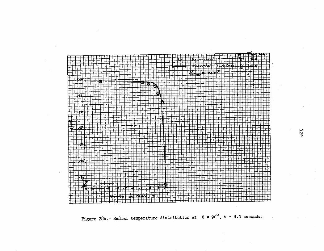
12
2
0co
ao00 oCI
C)0 r orI
4oa0p40as
Ca
Fx4
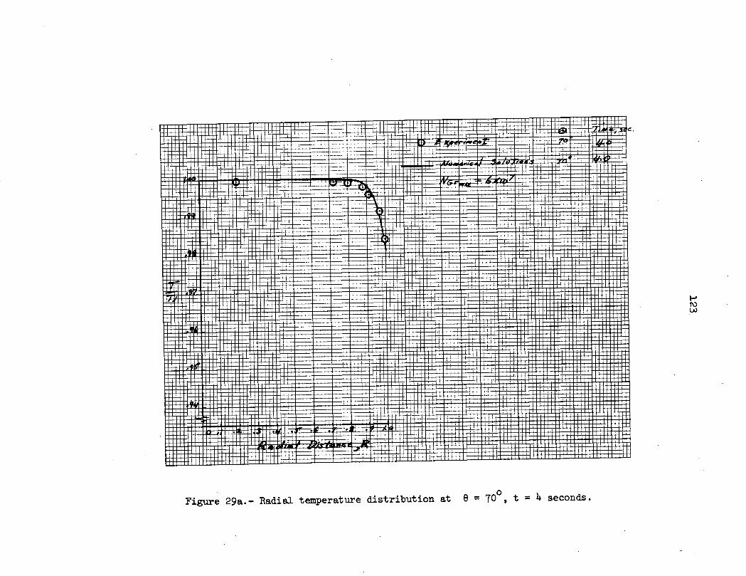
123
k
0ooar
II
0oC
D
it ill
F
It 1
1t$$iII- ij i i 2I -
· i
fIt
.I 4)ta)P4
.r'ca,0\
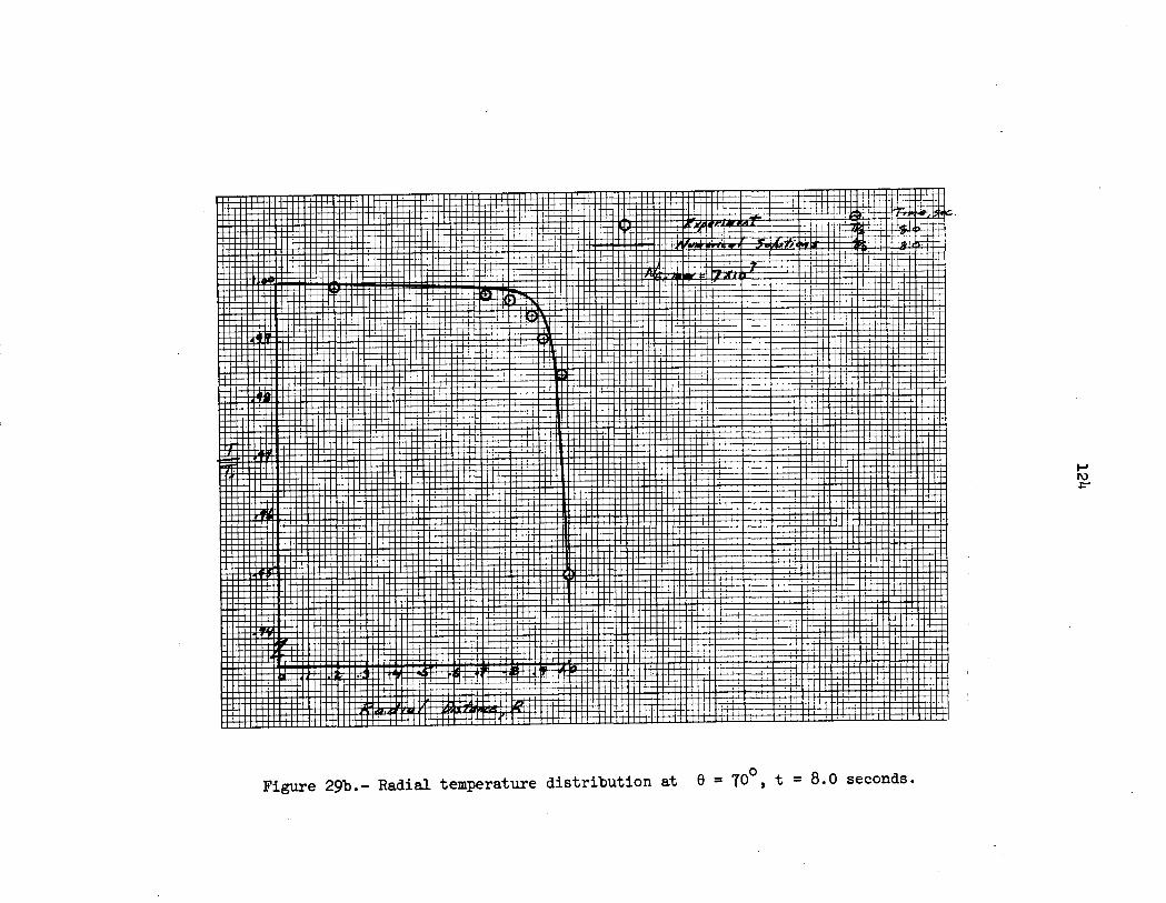
124
0Io 0o0ocoII4-
0oCMo1
CD00ci)'-4r4cm
.1jpt4
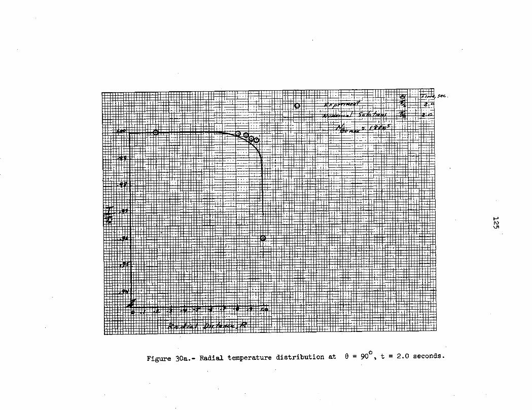
4R
I-4F
i
I-I ll-l .-
h l
ll ll
125
IaoC)
0 u,rCt00 II00 Ca
p,
.H4')
IdHo
asl
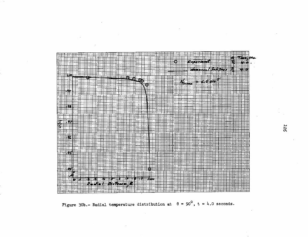
126
o Id
00Uo
oaNo
4.)
0
0,.,od Id0.,Ird
I ,,
,, M
1
, I., I
I, ,
, ,1
,
1 ,
,,, i.llz
, I
I .,
I ,
, ,
l
.. .............. ..............
Afitll
--------
P't --444--
----
---
------------+
++
4-� #4
i i ii
------ -------
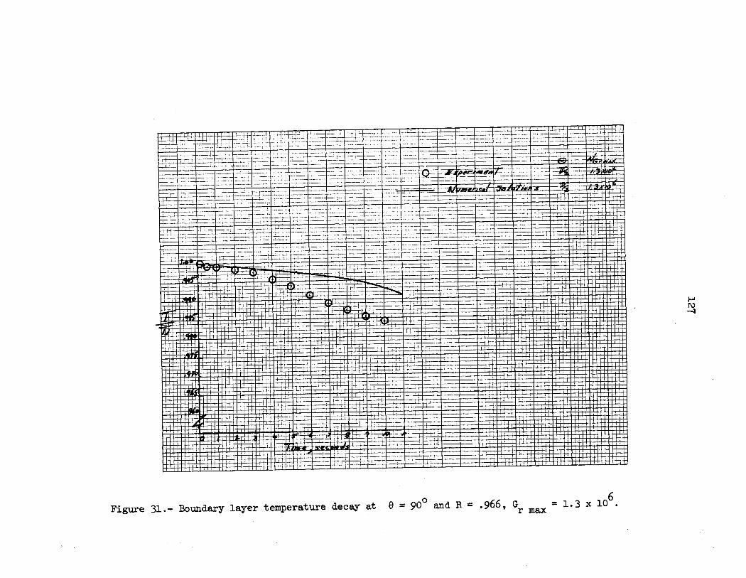
4EtRHit- i.!
i i f
1Si~t1|X1 JI
IIIIItI t
~ l
tV f-
: 111-11014:I
ii 4
, i ii
i t'
11i i 11
ii!~,1
S!1
. ·
!: m..
'tJt .
..
..
....-X
VFffill
'! i- I
' I
I |-
j It
Ii, I
! I 1ttltti l ll
Jt, tl- tti 1 1 t
I II liiM
It:'" ~ '
~" I Il
!i ..
... '?i
H I
~i. .
i !
ii .
..
rt!~, t'
;- -
~tti~
~~
~~
~~
~1
,1 i I
, -....
t!!-!: ;ih-!
127
'o
II o
$4
0o II,-0II o0
<D0a0 a0el
~'i~~i- i ~ll
"!it I
im
t' i!
i ! -
i i
I ~ '
1:I- iii:
:I!
-r L''
1 Z
1
1 1i
I I if Z
I IZI ii
Tf 1
1''
1 11
iSl( -
l-l ii L
lllllliqtllt
I;I -1-i1_j71
-1711:1III E
i ii-,: !+ -{ ~!
t 4-! .Iu
I .I
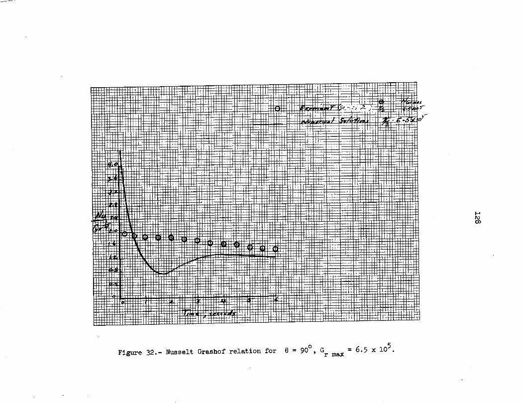
128
oU'N0Hx'l-o0\II 0oq.a.,l 0 r-I0 02
.rl.-
0)I o04rl
H,
wr
VITA
The author was born 2.
After moving to Seattle, Washington in 1938 he graduated from Garfield
High School in Seattle. Two years after entering the University of
Washington he entered the Naval Aviation Training program and in 1954
earned his commission and Naval aviators wings. For two and one half
years he flew with an operational Marine Jet fighter squadron. Follow-
ing completion of military service the author enrolled in the University
of Colorado School of Engineering. In 1960 had earned a Bachelor of
Science degree in Aerospace Engineering from the University of Colorado
and in that same year began full time employment with the National
Aeronautics and Space Administration at the Langley Research Center.
Through the NASA cooperative study program, the author earned a Master
of Aerospace Engineering degree from the University of Virginia in 1964.
In September of 1968 the author entered graduate school at Virginia
Polytechnic Institute to begin study for the degree of Doctor of
Philosophy in Aerospace Engineering.
The author resides in Yorktown, Virginia with his wife, Patricia,
and three sons, Roger, Keith, and Gordon.
129