718 ieee transactions on pattern analysis and … and... · propose a complete human recognition...

Human Ear Recognition in 3DHui Chen, Student Member, IEEE, and Bir Bhanu, Fellow, IEEE

Abstract—Human ear is a new class of relatively stable biometrics that has drawn researchers’ attention recently. In this paper, we

propose a complete human recognition system using 3D ear biometrics. The system consists of 3D ear detection, 3D ear identification,

and 3D ear verification. For ear detection, we propose a new approach which uses a single reference 3D ear shape model and locates the

ear helix and the antihelix parts in registered 2D color and 3D range images. For ear identification and verification using range images, two

new representations are proposed. These include the ear helix/antihelix representation obtained from the detection algorithm and the

local surface patch (LSP) representation computed at feature points. A local surface descriptor is characterized by a centroid, a local

surface type, and a 2D histogram. The 2D histogram shows the frequency of occurrence of shape index values versus the angles

between the normal of reference feature point and that of its neighbors. Both shape representations are used to estimate the initial rigid

transformation between a gallery-probe pair. This transformation is applied to selected locations of ears in the gallery set and a modified

Iterative Closest Point (ICP) algorithm is used to iteratively refine the transformation to bring the gallery ear and probe ear into the best

alignment in the sense of the least root mean square error. The experimental results on the UCR data set of 155 subjects with 902 images

under pose variations and the University of Notre Dame data set of 302 subjects with time-lapse gallery-probe pairs are presented to

compare and demonstrate the effectiveness of the proposed algorithms and the system.

Index Terms—3D ear biometrics, 3D ear identification, 3D ear verification, range and color images, surface matching.

Ç

1 INTRODUCTION

BIOMETRICS deal with recognition of individuals based ontheir physiological or behavioral characteristics [1].

Researchers have done extensive studies on biometrics suchas fingerprint, face, palm print, iris, and gait. Ear, a viable newclass of biometrics, has certain advantages over face andfingerprint, which are the two most common biometrics inboth academic research and industrial applications. Forexample, the ear is rich in features; it is a stable structurethat does not change much with age [2] and it does not changeits shape with facial expressions. Furthermore, ear is larger insize compared to fingerprints but smaller as compared to faceand it can be easily captured from a distance without a fullycooperative subject although it can sometimes be hidden withhair, cap, turban, muffler, scarf, and earrings. The anatomicalstructure of the human ear is shown in Fig. 1. The ear is madeup of standard features like the face. These include the outerrim (helix) and ridges (antihelix) parallel to the helix, the lobe,the concha (hollow part of ear), and the tragus (the smallprominence of cartilage over the meatus). In this paper, weuse the helix/antihelix for ear recognition.

Researchers have developed several biometrics techni-ques using the 2D intensity images [1, chapter 13], [3], [4], [5].The performance of these techniques is greatly affected by thepose variation and imaging conditions. However, an ear canbe imaged in 3D using a range sensor which provides aregistered color and range image pair. Fig. 2 shows anexample of a range image and the registered color imageacquired by the Minolta Vivid 300 camera. A range image is

relatively insensitive to illuminations and it contains surfaceshape information related to the anatomical structure, whichmakes it possible to develop a robust 3D ear biometrics.Examples of ear recognition using 3D data are [6], [7], [8], [9],[10], [11], [12], [13]. More work on the 3D face biometrics canbe found in [14], [15], [16], [17], [18], [19], [20].

In this paper, we propose a complete human recognitionsystem using 3D ear biometrics. The system has two keycomponents: 3D ear detection and 3D ear recognition. For eardetection, we propose a two-step approach using theregistered 2D color and range images by locating the earhelix and the antihelix parts. In the first step, a skin colorclassifier is used to isolate the side face in an image bymodeling the skin color and nonskin color distributions as amixture of Gaussians [21]. The edges from the 2D color imageare combined with the step edges from the range image tolocate regions-of-interest (ROIs) which may contain an ear. Inthe second step, to locate the ear accurately, the reference3D ear shape model, which is represented by a set of discrete3D vertices on the ear helix and the antihelix parts, is adaptedto individual ear images by following a new global-to-localregistration procedure instead of training an active shapemodel [22] built from a large set of ears to learn the shapevariation. The DARCES (data-aligned rigidity-constrainedexhaustive search) algorithm [23], which can solve the3D rigid registration problem efficiently and reliably, withoutany initial estimation, is used to perform the global registra-tion. This is followed by the local deformation process whereit is necessary to preserve the structure of the reference earshape model since neighboring points cannot move inde-pendently under the deformation due to physical constraints.The bending energy of thin plate spline [24], a quantitativemeasure for nonrigid deformations, is incorporated into theproposed optimization formulation as a regularization termto preserve the topology of the ear shape model under theshape deformation. The optimization procedure drives theinitial global registration toward the ear helix and the

718 IEEE TRANSACTIONS ON PATTERN ANALYSIS AND MACHINE INTELLIGENCE, VOL. 29, NO. 4, APRIL 2007

. The authors are with the Center for Research in Intelligent Systems,University of California at Riverside, Riverside, CA 92521.E-mail: {hchen, bhanu}@cris.ucr.edu.

Manuscript received 2 Feb. 2006; revised 8 Aug. 2006; accepted 30 Oct. 2006;published online 18 Jan. 2007.Recommended for acceptance by S. Prabhakar, J. Kittler, D. Maltoni,L. O’Gorman, and T. TanFor information on obtaining reprints of this article, please send e-mail to:[email protected] and reference IEEECSLog Number TPAMISI-0116-0206.Digital Object Identifier no. 10.1109/TPAMI.2007.1005.

0162-8828/07/$25.00 � 2007 IEEE Published by the IEEE Computer Society

antihelix parts, which results in the one-to-one correspon-dence of the ear helix and the antihelix between the referenceear shape model and the input image.

The approach for ear detection is followed to build adatabase of ears that belong to different people. For earrecognition, we present two representations: the ear helix/antihelix representation obtained from the detection algo-rithm and a new local surface patch representation computedat feature points to estimate the initial rigid transformationbetween a gallery-probe pair. For the ear helix/antihelixrepresentation, the correspondence of ear helix and antihelixparts (available from the ear detection algorithm) between agallery-probe ear pair is established and it is used to computethe initial rigid transformation. For the local surface patch(LSP) representation, a local surface descriptor is character-ized by a centroid, a local surface type, and a 2D histogram.The local surface descriptors are computed for the featurepoints, which are defined as either the local minimum or thelocal maximum of shape indexes. By comparing the localsurface patches for a gallery and a probe image, the potentialcorresponding local surface patches are established and thenfiltered by geometric constraints. Based on the filteredcorrespondences, the initial rigid transformation is esti-mated. Once this transformation is obtained using either ofthe two representations, it is then applied to randomlyselected control points of the hypothesized gallery ear in thedatabase. A modified Iterative Closest Point (ICP) algorithmis run to improve the transformation, which brings a galleryear and a probe ear into the best alignment, for every gallery-probe pair. The root mean square (RMS) registration error isused as the matching error criterion. The subject in the gallerywith the minimum RMS error is declared as the recognizedperson in the probe image.

The rest of the paper is organized as follows: Section 2introduces the related work and the contributions. Section 3presents the ear recognition system. It presents the two-stepapproach to automatically detect ears using side face colorand range images and describes the surface matchingscheme to recognize ears using the ear helix/antihelixrepresentation and the local surface patch representation.Section 4 develops a model to predict the performance ofthe ear recognition system in terms of cumulative matchcharacteristic (CMC) curve. Section 5 gives the experimentalresults to demonstrate the effectiveness of the proposedapproaches and the performance of the system. Finally,Section 6 provides the conclusions. Additional results areprovided in the supplemental material [25].

2 RELATED WORK AND CONTRIBUTIONS

2.1 Related Work

Detection and recognition are the two major components of abiometrics system. Tables 1 and 2 provide a summary ofobject detection and recognition approaches for 3D bio-metrics. Table 3 compares our approach with Yan andBowyer’s work [8], [9], [10], [11], [12], [13] which is close toour research. As compared to all the work presented inTables 1, 2, and 3, the detection approach proposed here usesa single reference ear shape model and exploits a two-stepprocedure that includes fusion of color and range data and thesystematic adaptation of the shape model for local deforma-tion. For the recognition, the most important differencebetween our approach and their work [8], [9], [10], [11], [12],[13] is that this paper proposes new ear helix/antihelix and

CHEN AND BHANU: HUMAN EAR RECOGNITION IN 3D 719

Fig. 1. The external ear and its anatomical parts.Fig. 2. Range image and color image captured by a Minolta Vivid 300

camera. In images (a) and (b), the range image of one ear is displayed as

the shaded mesh from two viewpoints (the units of X, Y, and Z are mm).

Image (c) shows the color image of the ear.

TABLE 1Object Detection: Summary of Approaches for 3D Biometrics

the local surface patch (LSP) representations to estimate the

initial rotation and translation between a gallery-probe pair.

The initial transformation is critical for the success of the ICP

algorithm and more details about it are given in Section 5.3.4.

2.2 Contributions of This Paper

The specific contributions of this paper are:

1. An automatic human recognition system using the3D ear biometrics is developed.

2. A single reference ear shape model is adapted toincoming images by following a new global-to-localregistration procedure with an associated optimiza-tion formulation. The bending energy of thin platespline is incorporated into the optimization formula-tion as a regularization term to preserve the structureof the reference shape model under the deformation.This formulation can be applied to handle thenonrigid shape registration and it is demonstratedfor the alignment of the hand and dude shapes.

3. The helix/antihelix-based representation and the invar-iant local surface patch representation for recognizingears in 3D are proposed. These representations areevaluated for their pose invariance and robustness tothe real world data.

4. A simple and effective surface matching schemebased on the modified ICP algorithm is introduced.ICP is initialized by a full 3D (translation androtation) transformation.

5. A binomial model is presented for characterizing theperformance of ear recognition.

6. The experimental results on two large ear databases(UCR and UND databases) of color and rangeimages are presented and compared with the otherpublished work [8], [9], [10], [11], [12], [13].

3 TECHNICAL APPROACH

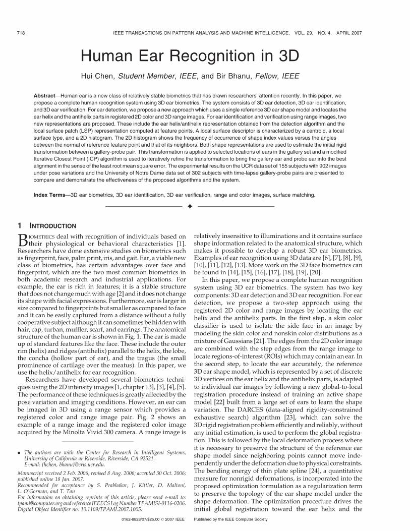
The proposed human recognition system using 3D earbiometrics is illustrated in Fig. 3. It consists of twocomponents: 3D ear detection and 3D ear recognition. Byfollowing the ear detection algorithm, ears are automaticallyextracted in side face range images. For the ear helix/antihelix representation, the ear gallery consists of 3D rangedata associated with the 3D coordinates of ear helix andantihelix parts obtained in detection. For the local surfacepatch (LSP) representation, the ear gallery consists of a set ofdescriptors associated with 3D range data. They are com-puted at selected feature points marked by plus signs in Fig. 3.In the following, we describe the details of the proposed eardetection and recognition algorithms and the system.


TABLE 2Object Recognition: Summary of Approaches for 3D Biometrics

TABLE 3Comparison between Chen and Bhanu’s and Yan and Bowyer’s Approaches in Methodology

3.1 Automatic Ear Extraction

The Minolta Vivid 300 and 910 range sensors used in thiswork provide a registered 3D range image and a 2D colorimage. The ear detection starts with the extraction of regions-of-interest (ROIs) using both the range and color images.Once the ROIs are located, the problem of identifying the earhelix and antihelix parts in a range image is converted to thealignment of the reference ear shape model with ROIs. Thealignment follows a new global-to-local procedure: Theglobal registration brings the reference shape model intocoarse alignment with the ear helix and the antihelix parts; thelocal deformation driven by the optimization formulationdrives the shape model more close to the ear helix and theantihelix parts.

3.1.1 Regions-of-Interest (ROIs) Extraction

Since the images in two modalities (range and color) areregistered, the ROIs can be localized in any one modality ifthey are known in the other modality.

. Processing Color Images. The processing consists oftwo major tasks:

- Skin Color Classification. Skin color is a power-ful cue for segmenting the exposed parts of thehuman body. Jones and Rehg [21] built a classifierby learning the distributions of skin and nonskinpixels from a data set of nearly one billion labeledpixels. The distributions are modeled as a mixtureof Gaussians and their parameters are given in[21]. We use this method for finding skin regions.

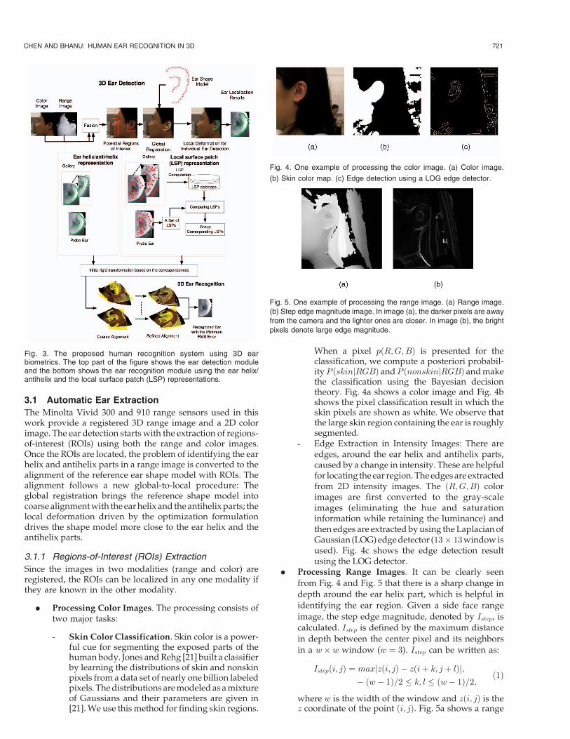
When a pixel pðR;G;BÞ is presented for theclassification, we compute a posteriori probabil-ityP ðskinjRGBÞ andP ðnonskinjRGBÞ and makethe classification using the Bayesian decisiontheory. Fig. 4a shows a color image and Fig. 4bshows the pixel classification result in which theskin pixels are shown as white. We observe thatthe large skin region containing the ear is roughlysegmented.

- Edge Extraction in Intensity Images: There areedges, around the ear helix and antihelix parts,caused by a change in intensity. These are helpfulfor locating the ear region. The edges are extractedfrom 2D intensity images. The ðR;G;BÞ colorimages are first converted to the gray-scaleimages (eliminating the hue and saturationinformation while retaining the luminance) andthen edges are extracted by using the Laplacian ofGaussian (LOG) edge detector (13� 13 window isused). Fig. 4c shows the edge detection resultusing the LOG detector.

. Processing Range Images. It can be clearly seen

from Fig. 4 and Fig. 5 that there is a sharp change in

depth around the ear helix part, which is helpful in

identifying the ear region. Given a side face range

image, the step edge magnitude, denoted by Istep, iscalculated. Istep is defined by the maximum distance

in depth between the center pixel and its neighbors

in a w� w window (w ¼ 3). Istep can be written as:

Istepði; jÞ ¼ maxjzði; jÞ � zðiþ k; jþ lÞj;� ðw� 1Þ=2 � k; l � ðw� 1Þ=2;

ð1Þ

where w is the width of the window and zði; jÞ is thez coordinate of the point ði; jÞ. Fig. 5a shows a range


Fig. 3. The proposed human recognition system using 3D earbiometrics. The top part of the figure shows the ear detection moduleand the bottom shows the ear recognition module using the ear helix/antihelix and the local surface patch (LSP) representations.

Fig. 4. One example of processing the color image. (a) Color image.

(b) Skin color map. (c) Edge detection using a LOG edge detector.

Fig. 5. One example of processing the range image. (a) Range image.

(b) Step edge magnitude image. In image (a), the darker pixels are away

from the camera and the lighter ones are closer. In image (b), the bright

pixels denote large edge magnitude.

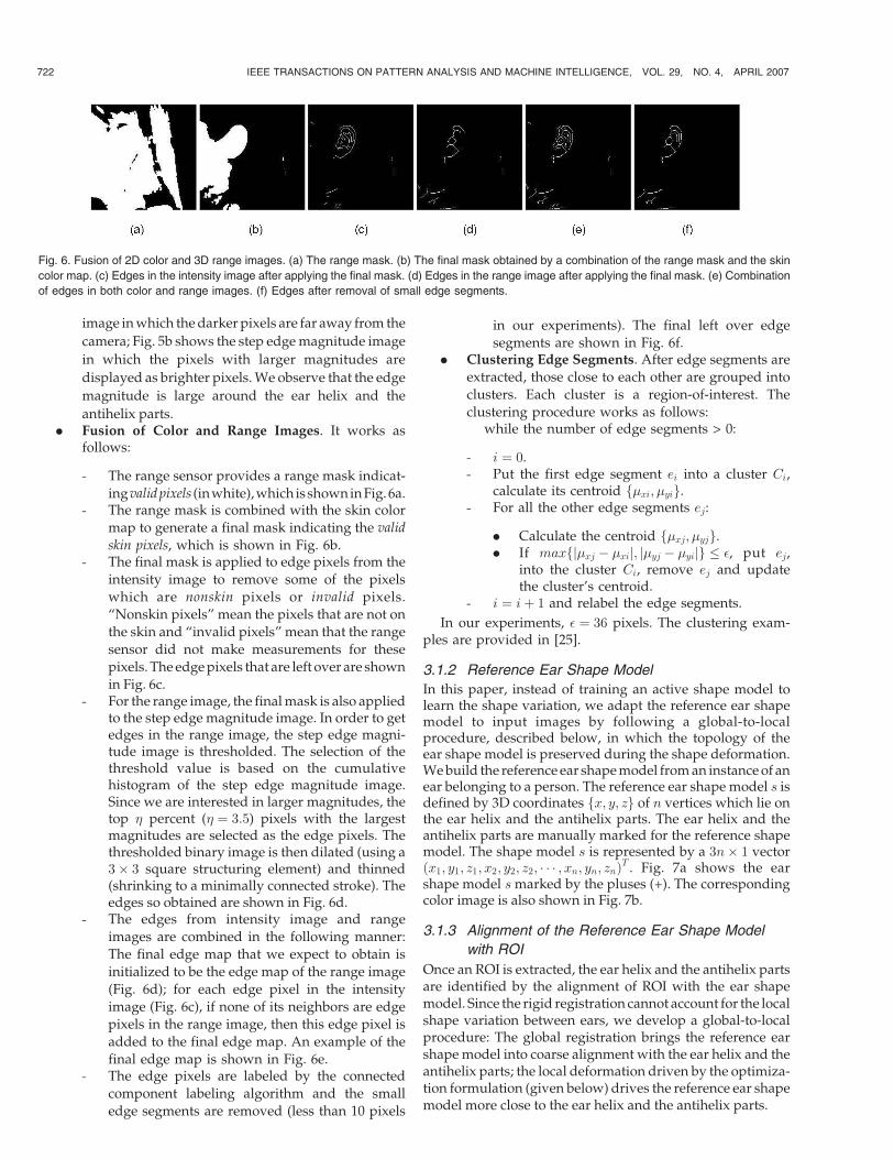
image in which the darker pixels are far away from the

camera; Fig. 5b shows the step edge magnitude image

in which the pixels with larger magnitudes are

displayed as brighter pixels. We observe that the edge

magnitude is large around the ear helix and the

antihelix parts.. Fusion of Color and Range Images. It works as

follows:

- The range sensor provides a range mask indicat-

ingvalidpixels (inwhite), whichisshowninFig.6a.- The range mask is combined with the skin color

map to generate a final mask indicating the valid

skin pixels, which is shown in Fig. 6b.- The final mask is applied to edge pixels from the

intensity image to remove some of the pixels

which are nonskin pixels or invalid pixels.“Nonskin pixels” mean the pixels that are not on

the skin and “invalid pixels” mean that the range

sensor did not make measurements for these

pixels. The edge pixels that are left over are shown

in Fig. 6c.- For the range image, the final mask is also applied

to the step edge magnitude image. In order to getedges in the range image, the step edge magni-tude image is thresholded. The selection of thethreshold value is based on the cumulativehistogram of the step edge magnitude image.Since we are interested in larger magnitudes, thetop � percent (� ¼ 3:5) pixels with the largestmagnitudes are selected as the edge pixels. Thethresholded binary image is then dilated (using a3� 3 square structuring element) and thinned(shrinking to a minimally connected stroke). Theedges so obtained are shown in Fig. 6d.

- The edges from intensity image and range

images are combined in the following manner:

The final edge map that we expect to obtain is

initialized to be the edge map of the range image

(Fig. 6d); for each edge pixel in the intensity

image (Fig. 6c), if none of its neighbors are edgepixels in the range image, then this edge pixel is

added to the final edge map. An example of the

final edge map is shown in Fig. 6e.- The edge pixels are labeled by the connected

component labeling algorithm and the small

edge segments are removed (less than 10 pixels

in our experiments). The final left over edgesegments are shown in Fig. 6f.

. Clustering Edge Segments. After edge segments are

extracted, those close to each other are grouped into

clusters. Each cluster is a region-of-interest. The

clustering procedure works as follows:while the number of edge segments > 0:

- i ¼ 0.- Put the first edge segment ei into a cluster Ci,

calculate its centroid f�xi; �yig.- For all the other edge segments ej:

. Calculate the centroid f�xj; �yjg.

. If maxfj�xj � �xij; j�yj � �yijg � �, put ej,into the cluster Ci, remove ej and updatethe cluster’s centroid.

- i ¼ iþ 1 and relabel the edge segments.

In our experiments, � ¼ 36 pixels. The clustering exam-ples are provided in [25].

3.1.2 Reference Ear Shape Model

In this paper, instead of training an active shape model tolearn the shape variation, we adapt the reference ear shapemodel to input images by following a global-to-localprocedure, described below, in which the topology of theear shape model is preserved during the shape deformation.We build the reference ear shape model from an instance of anear belonging to a person. The reference ear shape model s isdefined by 3D coordinates fx; y; zg of n vertices which lie onthe ear helix and the antihelix parts. The ear helix and theantihelix parts are manually marked for the reference shapemodel. The shape model s is represented by a 3n� 1 vectorðx1; y1; z1; x2; y2; z2; � � � ; xn; yn; znÞT . Fig. 7a shows the earshape model s marked by the pluses (+). The correspondingcolor image is also shown in Fig. 7b.

3.1.3 Alignment of the Reference Ear Shape Model

with ROI

Once an ROI is extracted, the ear helix and the antihelix partsare identified by the alignment of ROI with the ear shapemodel. Since the rigid registration cannot account for the localshape variation between ears, we develop a global-to-localprocedure: The global registration brings the reference earshape model into coarse alignment with the ear helix and theantihelix parts; the local deformation driven by the optimiza-tion formulation (given below) drives the reference ear shapemodel more close to the ear helix and the antihelix parts.


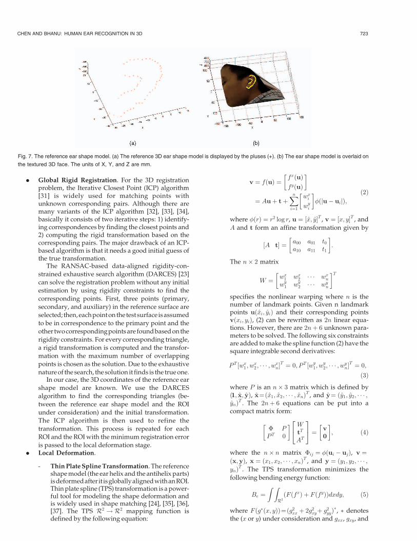
Fig. 6. Fusion of 2D color and 3D range images. (a) The range mask. (b) The final mask obtained by a combination of the range mask and the skin

color map. (c) Edges in the intensity image after applying the final mask. (d) Edges in the range image after applying the final mask. (e) Combination

of edges in both color and range images. (f) Edges after removal of small edge segments.

. Global Rigid Registration. For the 3D registrationproblem, the Iterative Closest Point (ICP) algorithm[31] is widely used for matching points withunknown corresponding pairs. Although there aremany variants of the ICP algorithm [32], [33], [34],basically it consists of two iterative steps: 1) identify-ing correspondences by finding the closest points and2) computing the rigid transformation based on thecorresponding pairs. The major drawback of an ICP-based algorithm is that it needs a good initial guess ofthe true transformation.

The RANSAC-based data-aligned rigidity-con-

strained exhaustive search algorithm (DARCES) [23]

can solve the registration problem without any initial

estimation by using rigidity constraints to find the

corresponding points. First, three points (primary,

secondary, and auxiliary) in the reference surface are

selected; then, eachpointon thetest surface is assumed

to be in correspondence to the primary point and the

other twocorrespondingpoints are foundbasedon the

rigidity constraints. For every corresponding triangle,

a rigid transformation is computed and the transfor-

mation with the maximum number of overlapping

points is chosen as the solution. Due to the exhaustive

nature of the search, the solution it finds is the true one.In our case, the 3D coordinates of the reference ear

shape model are known. We use the DARCES

algorithm to find the corresponding triangles (be-

tween the reference ear shape model and the ROI

under consideration) and the initial transformation.

The ICP algorithm is then used to refine the

transformation. This process is repeated for each

ROI and the ROI with the minimum registration error

is passed to the local deformation stage.. Local Deformation.

- Thin Plate Spline Transformation. The referenceshape model (the ear helix and the antihelix parts)isdeformedafter it isgloballyalignedwithanROI.Thin plate spline (TPS) transformation is a power-ful tool for modeling the shape deformation andis widely used in shape matching [24], [35], [36],[37]. The TPS R2 !R2 mapping function isdefined by the following equation:

v ¼ fðuÞ ¼fxðuÞfyðuÞ

� �¼ Auþ tþ

Xni¼1

wxiwyi

� ��ðju� uijÞ;

ð2Þ

where �ðrÞ ¼ r2 log r, u ¼ ½x; y�T , v ¼ ½x; y�T , and

A and t form an affine transformation given by

½A t� ¼ a00 a01 t0a10 a11 t1

� �:

The n� 2 matrix

W ¼ wx1 wx2 � � � wxnwy1 wy2 � � � wyn

� �Tspecifies the nonlinear warping where n is thenumber of landmark points. Given n landmarkpoints uðxi; yiÞ and their corresponding pointsvðxi; yiÞ, (2) can be rewritten as 2n linear equa-tions. However, there are 2nþ 6 unknown para-meters to be solved. The following six constraintsare added to make the spline function (2) have thesquare integrable second derivatives:

PT ½wx1 ; wx2 ; � � � ; wxn�T ¼ 0; PT ½wy1; w

y2; � � � ; wyn�

T ¼ 0;

ð3Þ

where P is an n� 3 matrix which is defined byð1; x; yÞ, x¼ðx1; x2; � � � ; xnÞT , and y¼ ðy1; y2; � � � ;ynÞT . The 2nþ 6 equations can be put into acompact matrix form:

� PPT 0

� � WtT

AT

24 35 ¼ v0

� �; ð4Þ

where the n� n matrix �ij ¼ �ðui � ujÞ, v ¼ðx;yÞ, x ¼ ðx1; x2; � � � ; xnÞT , and y ¼ ðy1; y2; � � � ;ynÞT . The TPS transformation minimizes the

following bending energy function:

Be ¼Z Z

R2ðF ðfxÞ þ F ðfyÞÞdxdy; ð5Þ

where F ðg�ðx; yÞÞ¼ðg2xx þ 2g2

xyþ g2yyÞ�, � denotes

the (x or y) under consideration and gxx, gxy, and


Fig. 7. The reference ear shape model. (a) The reference 3D ear shape model is displayed by the pluses (+). (b) The ear shape model is overlaid on

the textured 3D face. The units of X, Y, and Z are mm.

gyy are second order derivatives. It can be shownthat the value of bending energy is Be ¼ 1

8�

ðxTKxþ yTKyÞ, where x¼ ðx1; x2; � � � ; xnÞT andy ¼ ðy1; y2; � � � ; ynÞT [24]. The matrix K is then� n upper left matrix of

� PPT 0

� ��1

;

which only depends on the coordinates of thelandmark points in fug. Therefore, the bendingenergy is determined by the coordinates oflandmark points and their correspondences.Furthermore, the bending energy is a goodmeasurement of the shape deformation. Sincethe coordinates of the reference ear shape modelare known, the matrix K can be precomputed.The task is to drive the reference ear shape modeltoward the ROI ear such that the topology of thereference ear shape model is preserved. Thebending energy is used to penalize the largeshape deformation.

- Optimization Formulation. In Section 3.1.1, wenoted that there are strong step edge magnitudesin range images around the ear helix and theantihelix parts. After we bring the referenceshape model into coarse alignment with the earhelix and the antihelix parts (in the ROI image)through the global rigid registration, we get thelocations of the 3D coordinates of ear helix andantihelix parts in the 2D color image and performthe local deformation on the 2D image planesince the 2D color image is registered with the3D range image. In other words, we would like todrive the reference ear shape model more close tothe ear helix and the antihelix parts with thetopology of the shape model preserved. We canachieve this task by minimizing the proposednew cost function:

Eðx;yÞ ¼ Eimgðx;yÞ þ �EDðx;yÞ

¼Xni¼1

hðjrIstepðxi; yiÞjÞ

þ 1

2�ðxTKxþ yTKyÞ;

ð6Þ

where hðjrIstepjÞ¼1=ð1þ jrIstepjÞ, jrIstep ðxi; yiÞjis the step edgemagnitudeof ithpoint of the shapemodel located in the 2D plane and � is a positiveregularization constant that controls the topologyof the shape model. For example, increasing themagnitude of � tends to keep the topology of theear shape model unchanged. In (6), the step edgemagnitude in range images is used for the termEimg since edges in range images are less sensitiveto the change of viewpoint and illumination thanthose in color images. In (6), the first term Eimg

drives points (x;yÞ toward the ear helix and theantihelix parts which have larger step edgemagnitudes; the second term ED is the bendingenergy that preserves the topology of the refer-ence shape model under the shape deformation.

When we take the partial derivatives of (6) withrespect to x and y and set them to zero, we have

�Kx�Xni¼1

1

ð1þ jrIstepðxi; yiÞjÞ2@jrIstepðxi; yiÞj

@x¼ 0;

�Ky�Xni¼1

1

ð1þ jrIstepðxi; yiÞjÞ2@jrIstepðxi; yiÞj

@y¼ 0:

ð7Þ

Since K is positive semidefinite, (7) can besolved iteratively by introducing a step sizeparameter �, which is shown in (8) [38].

�Kxt þ �ðxt � xt�1Þ � Fxt�1 ¼ 0;

�Kyt þ �ðyt � yt�1Þ � Fyt�1 ¼ 0: ð8Þ

The solutions can be obtained by matrix inver-

sion, which is shown in (9), where I is theidentity matrix. In (8) and (9),

Fxt�1 ¼

Xni¼1

1

ð1þ jrIt�1stepðxi; yiÞjÞ

2

@jrIt�1stepðxi; yiÞj@x

and

Fyt�1 ¼

Xni¼1

1

ð1þ jrIt�1stepðxi; yiÞjÞ

2

@jrIt�1stepðxi; yiÞj@y

;

and they are evaluated for all the coordinatesðxi; yiÞ at the iteration t� 1. jrIt�1

stepðxi; yiÞj is thestep edge magnitude at the location ðxi; yiÞ at theiteration t� 1.

xt ¼ ð�K þ �IÞ�1��xt�1 þ Fx

t�1

�;

yt ¼ ð�K þ �IÞ�1��yt�1 þ F

yt�1

�:

ð9Þ

We have used � ¼ 0:5 and � ¼ 100 in our experiments onear detection described in Section 5.

3.2 Surface Matching for Ear Recognition Using theEar Helix/Antihelix Representation

As shown in the ear recognition part of Fig. 3, the surfacematching follows the coarse-to-fine strategy. Given a set ofprobe images, the ear and its helix and the antihelix partsare extracted by running the detection algorithm describedabove. The correspondence of the helix and the antihelixbetween the probe ear and the hypothesized gallery ear isused to compute the initial transformation that brings thehypothesized gallery ear into coarse alignment with theprobe ear and then a modified ICP algorithm is run to refinethe transformation to bring gallery-probe pairs into the bestalignment.

3.2.1 Coarse Alignment

Given two corresponding sets ofn 3D verticesM andS on thehelix and the antihelix parts, the initial rigid transformation,


which brings the gallery and the probe ears into coarsealignment, can be estimated by minimizing the sum of thesquares of theses errors (� ¼ 1

n

Pnl¼1 jSl �R �Ml � T j2) with

respect to the rotation matrix R and the translation vector T .The rotation matrix and translation vector are computed byusing the quaternion representation [39].

3.2.2 Fine Alignment

Given the estimate of initial rigid transformation, the purposeof Iterative Closest Point (ICP) algorithm [31] is to determineif the match is good and to find a refined alignment betweenthem. If the probe ear is really an instance of the gallery ear,the ICP algorithm will result in good registration and a largenumber of corresponding points between gallery and probeear surfaces will be found. Since ICP algorithm requires thatthe probe be a subset of the gallery, a method to removeoutliers based on the distance distribution is used [33]. Thebasic steps of the modified ICP algorithm are summarizedbelow:

. Input: A 3D gallery ear range image, a 3D probe earrange image, and the initial transformation obtainedfrom the coarse alignment.

. Output: The refined transformation between the twoears.

. Procedure:

a. Select control points (� 180) in the gallery earrange image randomly and apply the initialtransformation to the gallery ear image.

b. Find the closest points of the control points inthe probe ear image and compute the statistics[33] of the distances between the correspondingpairs in the gallery and the probe images.

c. Discard some of the corresponding pairs byanalyzing the statistics of the distances (athreshold is obtained based on the mean andstandard deviation of distances) [33].

d. Compute the rigid transformation between thegallery and the probe ears based on thecorrespondences.

e. Apply the transformation to the gallery ear rangeimage and repeat from Step b until convergence.

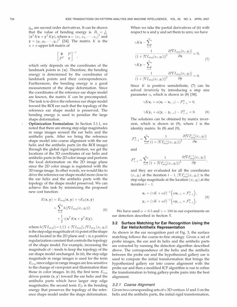
Starting with the initial transformation obtained from thecoarse alignment, the modified ICP algorithm is run to refinethe transformation by minimizing the distance between thecontrol points of the gallery ear and their closest points of theprobe ear. For each gallery ear in the database, the controlpoints are randomly selected and the modified ICP is appliedto those points. For a selected gallery ear, we repeat the sameprocedure 15 times and choose the rigid transformation withthe minimum root mean square (RMS) error. The subject inthe gallery set with the minimum RMS error is declared as therecognized person. In the modified ICP algorithm, the speedbottleneck is the nearest neighbor search. Therefore, thekd-tree structure is used in the implementation. Fig. 8a showsthe coarse alignment after applying the initial rigid transfor-mation; Fig. 8b shows the refined alignment after applyingthe modified ICP algorithm. In Fig. 8, the gallery earrepresented by the mesh is overlaid on the textured3D probe ear. We observe a better alignment after applyingthe modified ICP algorithm.

3.3 Surface Matching for Ear Recognition UsingLocal Surface Patch (LSP) Representation

In 3D object recognition, the key problems are how torepresent free-form surfaces effectively and how to matchthe surfaces using the selected representation. Researchershave proposed various surface signatures for recognizing3D free-form objects which are reviewed in [6], [40]. In thefollowing, we present a new surface representation, calledthe local surface patch (LSP), investigate its properties, anduse it for ear recognition.

3.3.1 Local Surface Patch Representation (LSP)

We define a “local surface patch” as the region consisting ofa feature point P and its neighbors N. The LSP representa-tion includes feature point P , its surface type, centroid ofthe patch, and a histogram of shape index values versus dotproduct of the surface normal at point P and its neighbors.A local surface patch is shown in Fig. 10. The neighborssatisfy the following conditions, N ¼ fpixels N; jjN �P jj � �1g and acosðnpnn < AÞ, where denotes the dotproduct between the surface normal vectors np and nn atpoint P and N and acos denotes the inverse cosine function.The two parameters �1 and A (�1 ¼ 5:8mm, A ¼ 0:5) areimportant since they determine the descriptiveness of thelocal surface patch representation. A local surface patch isnot computed at every pixel in a range image, but only atselected feature points. The feature points are defined as thelocal minimum and the maximum of shape indexes, whichcan be calculated from principal curvatures. In order toestimate curvatures, we fit a biquadratic surface fðx; yÞ ¼ax2 þ by2 þ cxyþ dxþ eyþ f to a local window and use theleast square method to estimate the parameters of thequadratic surface and then use differential geometry tocalculate the surface normal, Gaussian, and mean curva-tures and the principal curvatures [6], [41].

Shape index (Si), a quantitative measure of the shapeof a surface at a point P , is defined by

SiðP Þ ¼1

2� 1

�tan�1 k1ðP Þ þ k2ðP Þ

k1ðP Þ � k2ðP Þ;

where k1 and k2 are maximum and minimum principalcurvatures, respectively. With this definition, all shapes are


Fig. 8. Two examples of coarse and fine alignment. The gallery ear

represented by the mesh is overlaid on the textured 3D probe ear.

(a) Coarse alignment. (b) Fine alignment.

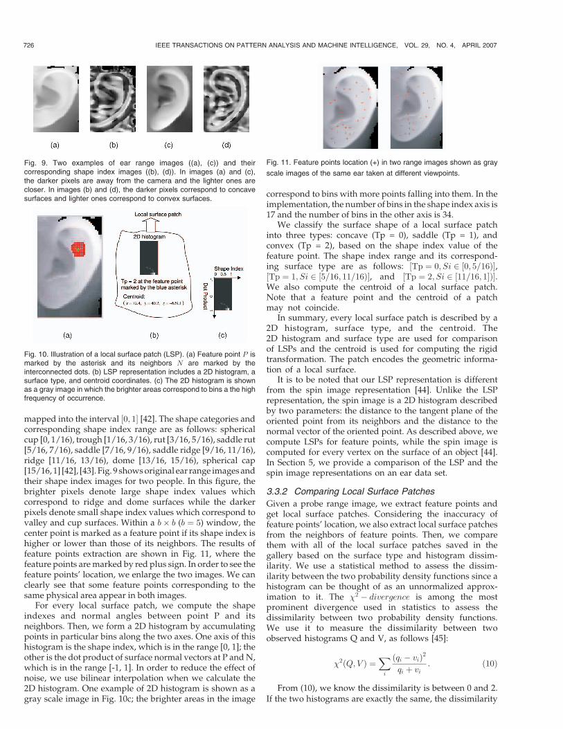
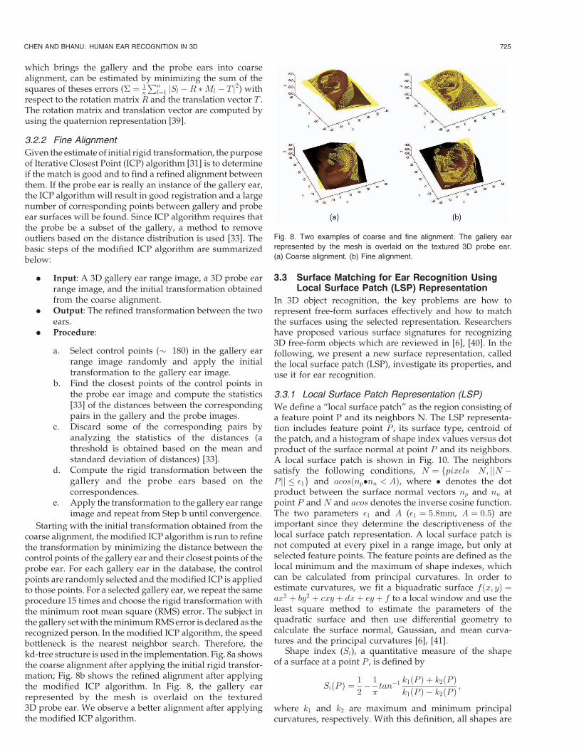
mapped into the interval ½0; 1� [42]. The shape categories andcorresponding shape index range are as follows: sphericalcup [0, 1/16), trough [1/16, 3/16), rut [3/16, 5/16), saddle rut[5/16, 7/16), saddle [7/16, 9/16), saddle ridge [9/16, 11/16),ridge [11/16, 13/16), dome [13/16, 15/16), spherical cap[15/16, 1] [42], [43]. Fig. 9 shows original ear range images andtheir shape index images for two people. In this figure, thebrighter pixels denote large shape index values whichcorrespond to ridge and dome surfaces while the darkerpixels denote small shape index values which correspond tovalley and cup surfaces. Within a b� b (b ¼ 5) window, thecenter point is marked as a feature point if its shape index ishigher or lower than those of its neighbors. The results offeature points extraction are shown in Fig. 11, where thefeature points are marked by red plus sign. In order to see thefeature points’ location, we enlarge the two images. We canclearly see that some feature points corresponding to thesame physical area appear in both images.

For every local surface patch, we compute the shapeindexes and normal angles between point P and itsneighbors. Then, we form a 2D histogram by accumulatingpoints in particular bins along the two axes. One axis of thishistogram is the shape index, which is in the range [0, 1]; theother is the dot product of surface normal vectors at P and N,which is in the range [-1, 1]. In order to reduce the effect ofnoise, we use bilinear interpolation when we calculate the2D histogram. One example of 2D histogram is shown as agray scale image in Fig. 10c; the brighter areas in the image

correspond to bins with more points falling into them. In theimplementation, the number of bins in the shape index axis is17 and the number of bins in the other axis is 34.

We classify the surface shape of a local surface patchinto three types: concave (Tp = 0), saddle (Tp = 1), andconvex (Tp = 2), based on the shape index value of thefeature point. The shape index range and its correspond-ing surface type are as follows: ½Tp ¼ 0; Si 2 ½0; 5=16Þ�,½Tp ¼ 1; Si 2 ½5=16; 11=16Þ�, and ½Tp ¼ 2; Si 2 ½11=16; 1�Þ�.We also compute the centroid of a local surface patch.Note that a feature point and the centroid of a patchmay not coincide.

In summary, every local surface patch is described by a2D histogram, surface type, and the centroid. The2D histogram and surface type are used for comparisonof LSPs and the centroid is used for computing the rigidtransformation. The patch encodes the geometric informa-tion of a local surface.

It is to be noted that our LSP representation is differentfrom the spin image representation [44]. Unlike the LSPrepresentation, the spin image is a 2D histogram describedby two parameters: the distance to the tangent plane of theoriented point from its neighbors and the distance to thenormal vector of the oriented point. As described above, wecompute LSPs for feature points, while the spin image iscomputed for every vertex on the surface of an object [44].In Section 5, we provide a comparison of the LSP and thespin image representations on an ear data set.

3.3.2 Comparing Local Surface Patches

Given a probe range image, we extract feature points andget local surface patches. Considering the inaccuracy offeature points’ location, we also extract local surface patchesfrom the neighbors of feature points. Then, we comparethem with all of the local surface patches saved in thegallery based on the surface type and histogram dissim-ilarity. We use a statistical method to assess the dissim-ilarity between the two probability density functions since ahistogram can be thought of as an unnormalized approx-imation to it. The 2 � divergence is among the mostprominent divergence used in statistics to assess thedissimilarity between two probability density functions.We use it to measure the dissimilarity between twoobserved histograms Q and V, as follows [45]:

2ðQ; V Þ ¼Xi

ðqi � viÞ2

qi þ vi: ð10Þ

From (10), we know the dissimilarity is between 0 and 2.If the two histograms are exactly the same, the dissimilarity


Fig. 9. Two examples of ear range images ((a), (c)) and theircorresponding shape index images ((b), (d)). In images (a) and (c),the darker pixels are away from the camera and the lighter ones arecloser. In images (b) and (d), the darker pixels correspond to concavesurfaces and lighter ones correspond to convex surfaces.

Fig. 10. Illustration of a local surface patch (LSP). (a) Feature point P ismarked by the asterisk and its neighbors N are marked by theinterconnected dots. (b) LSP representation includes a 2D histogram, asurface type, and centroid coordinates. (c) The 2D histogram is shownas a gray image in which the brighter areas correspond to bins a the highfrequency of occurrence.

Fig. 11. Feature points location (+) in two range images shown as gray

scale images of the same ear taken at different viewpoints.

will be zero. If the two histograms do not overlap with eachother, it will achieve the maximum value of 2.

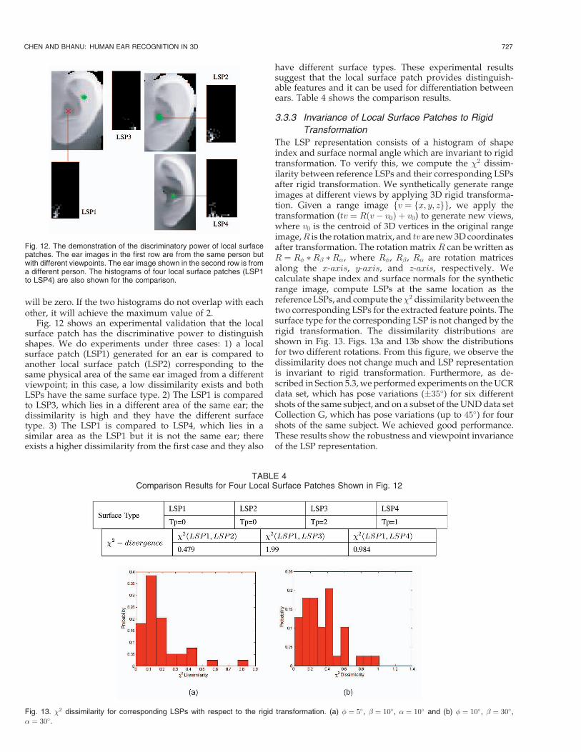
Fig. 12 shows an experimental validation that the localsurface patch has the discriminative power to distinguishshapes. We do experiments under three cases: 1) a localsurface patch (LSP1) generated for an ear is compared toanother local surface patch (LSP2) corresponding to thesame physical area of the same ear imaged from a differentviewpoint; in this case, a low dissimilarity exists and bothLSPs have the same surface type. 2) The LSP1 is comparedto LSP3, which lies in a different area of the same ear; thedissimilarity is high and they have the different surfacetype. 3) The LSP1 is compared to LSP4, which lies in asimilar area as the LSP1 but it is not the same ear; thereexists a higher dissimilarity from the first case and they also

have different surface types. These experimental resultssuggest that the local surface patch provides distinguish-able features and it can be used for differentiation betweenears. Table 4 shows the comparison results.

3.3.3 Invariance of Local Surface Patches to Rigid

Transformation

The LSP representation consists of a histogram of shapeindex and surface normal angle which are invariant to rigidtransformation. To verify this, we compute the 2 dissim-ilarity between reference LSPs and their corresponding LSPsafter rigid transformation. We synthetically generate rangeimages at different views by applying 3D rigid transforma-tion. Given a range image fv ¼ fx; y; zgg, we apply thetransformation (tv ¼ Rðv� v0Þ þ v0) to generate new views,where v0 is the centroid of 3D vertices in the original rangeimage,R is the rotation matrix, and tv are new 3D coordinatesafter transformation. The rotation matrix R can be written asR ¼ R� �R �R�, where R�, R, R� are rotation matricesalong the x-axis, y-axis, and z-axis, respectively. Wecalculate shape index and surface normals for the syntheticrange image, compute LSPs at the same location as thereference LSPs, and compute the2 dissimilarity between thetwo corresponding LSPs for the extracted feature points. Thesurface type for the corresponding LSP is not changed by therigid transformation. The dissimilarity distributions areshown in Fig. 13. Figs. 13a and 13b show the distributionsfor two different rotations. From this figure, we observe thedissimilarity does not change much and LSP representationis invariant to rigid transformation. Furthermore, as de-scribed in Section 5.3, we performed experiments on the UCRdata set, which has pose variations (35�) for six differentshots of the same subject, and on a subset of the UND data setCollection G, which has pose variations (up to 45�) for fourshots of the same subject. We achieved good performance.These results show the robustness and viewpoint invarianceof the LSP representation.


Fig. 12. The demonstration of the discriminatory power of local surfacepatches. The ear images in the first row are from the same person butwith different viewpoints. The ear image shown in the second row is froma different person. The histograms of four local surface patches (LSP1to LSP4) are also shown for the comparison.

TABLE 4Comparison Results for Four Local Surface Patches Shown in Fig. 12

Fig. 13. 2 dissimilarity for corresponding LSPs with respect to the rigid transformation. (a) � ¼ 5�, ¼ 10�, � ¼ 10� and (b) � ¼ 10�, ¼ 30�,

� ¼ 30�.

3.3.4 Grouping Corresponding Pairs of Local Surface

Patch

For every local surface patch from the probe ear, we choose

the local surface patch from the database with minimum

dissimilarity and the same surface type as the possible

corresponding patch. We filter the possible corresponding

pairs based on the geometric constraints given below:

dC1;C2¼ jdS1;S2

� dM1;M2j < �2 maxðdS1;S2

; dM1;M2Þ > �3; ð11Þ

where dS1;S2and dM1;M2

are the Euclidean distance betweencentroids of two surface patches. The first constraintguarantees that distances dS1;S2

and dM1;M2are consistent;

the second constraint removes the correspondences whichare too close. For two correspondences, C1 ¼ fS1;M1g andC2 ¼ fS2;M2g, where S is the probe surface patch and M isthe gallery surface patch, they should satisfy (11) if they areconsistent corresponding pairs. Therefore, we use simplegeometric constraints to partition the potential correspond-ing pairs into different groups. The larger the group is, themore likely it contains the true corresponding pairs.

Given a list of corresponding pairs L ¼ fC1; C2; . . . ; Cng,the grouping procedure for every pair in the list is asfollows: Initialize each pair of a group. For every group, addother pairs to it if they satisfy (11). Repeat the sameprocedure for every group. Sort the groups in the ascendingorder based on the size of groups. Select the groups on thetop of the list.

Fig. 14 shows one example of partitioning correspondingpairs into different groups. Fig. 14a shows the feature point

extraction results for a probe ear. Comparing the local surfacepatches with LSPs on the gallery ear, the initial correspond-ing pairs are shown in Fig. 14b, in which every pair isrepresented by the same number superimposed on the probe

and gallery images. We observe that both the true and falsecorresponding pairs are found. The examples of filteredgroups after applying the two geometric constraints (11) are

shown in Figs. 14c and 14d, respectively. We can see that thetrue corresponding pairs are obtained by comparing localsurface patches and using the simple geometric constraints.

Once the corresponding LSPs between the gallery and

probe are established, the initial rigid transformation isestimated and the coarse-to-fine surface matching strategy isfollowed (see Section 3.2). Note that, in the supplementalmaterial, Section C [25], which can be found at http://

computer.org/tpami/archives.htm, we provide a quantita-tive analysis of the effect of the generating parameters on thecomparison of LSPs, the robustness of LSPs with respect to

noise, and the impact of the number of LSPs in the probeimage on the matching performance.

4 PERFORMANCE PREDICTION

The prediction of the performance of a biometrics system isan important consideration in the real-world applications.


Fig. 14. Example of grouping corresponding LSPs for a pair of ears with a large pose variation. The probe ear is shown on the left image in (b), (c),and (d). (a) Feature points extraction from a probe ear. (b) Initial corresponding pairs. (c) Example of filtered corresponding pairs. (d) Example offiltered corresponding pairs.

Our mathematical prediction model is based on the

distribution of match and nonmatch scores [46], [47]. Let

msðxÞ and nsðxÞ denote the distributions of match and

nonmatch scores in which the match score is the score

computed from the true-matched pair and the nonmatch

score is the score computed from the false-matched pair. If

the match score is higher, the match is closer. The error

occurs when any given match score is less than any of the

nonmatch scores. The probability that the nonmatch score is

greater than or equal to the match score x is NSðxÞ. It is

given by NSðxÞ ¼R1x nsðtÞdt.

The probability that the match score x has rank r

exactly is given by the binomial probability distribution

CN�1r�1 ð1�NSðxÞÞ

N�rNSðxÞr�1. By integrating over all the

match scores, we getZ 1�1

CN�1r�1 ð1�NSðxÞÞ

N�rNSðxÞr�1msðxÞdx:

In theory, the match scores can be any value within

ð�1;1Þ. Therefore, the probability that the match score is

within rank r, which is the definition of a cumulative match

characteristic (CMC) curve, is

P ðN; rÞ ¼Xri¼1

Z 1�1

CN�1i�1 ð1�NSðxÞÞ

N�iNSðxÞi�1msðxÞdx:

ð12Þ

In the above equations, N is the size of large population

whose recognition performance needs to be estimated. Here,

we assume that the match score and nonmatch score are

independent and the match and nonmatch score distribu-

tions are the same for all the people. The small size gallery is

used to estimate distributions of msðxÞ and nsðxÞ.For the ear recognition case, every 3D ear in the probe set

is matched to every 3D ear in the gallery set and the RMS

registration error is calculated using the procedure de-

scribed in Section 3.2. This RMS registration error is used as

the matching score criterion.

5 EXPERIMENTAL RESULTS

5.1 Data

The experiments are performed on the data set collected by

us (UCR data set) and the University of Notre Dame publicdata set (UND data set).1 In the UCR data set, there is notime lapse between the gallery and probe for the samesubject, while there is a time lapse of a few weeks (on theaverage) in the UND data set.

5.1.1 UCR Data Set

The data are captured by Minolta Vivid 300 camera. Thiscamera uses the light-stripe method to emit a horizontal stripelight to the object and the reflected light is then converted by

triangulation into distance information. The camera outputs arange image and its registered color image in less than onesecond. The range image contains 200� 200 grid points andeach grid point has a 3D coordinate (x; y; z) and a set of color(r; g; b) values. During the acquisition, 155 subjects sit on a

chair about 0:55 � 0:75m from the camera in an indoor officeenvironment. The first shot is taken when a subject’s left sideface is approximately parallel to the image plane; two shotsare taken when the subject is asked to rotate his/her head to

the left and to the right side within 35� with respect to his/her torso. During this process, there could be some face tilt aswell, which is not measured. A total of six images per subjectare recorded. In total, 902 shots are used for the experimentssince some shots are not properly recorded. Every person has

at least four shots. The average number of points on the sideface scans is 23,205. There are three different poses in thecollected data: frontal, left, and right. Among the total155 subjects, there are 17 females; six subjects have earringsand 12 subjects have their ears partially occluded by hair (with

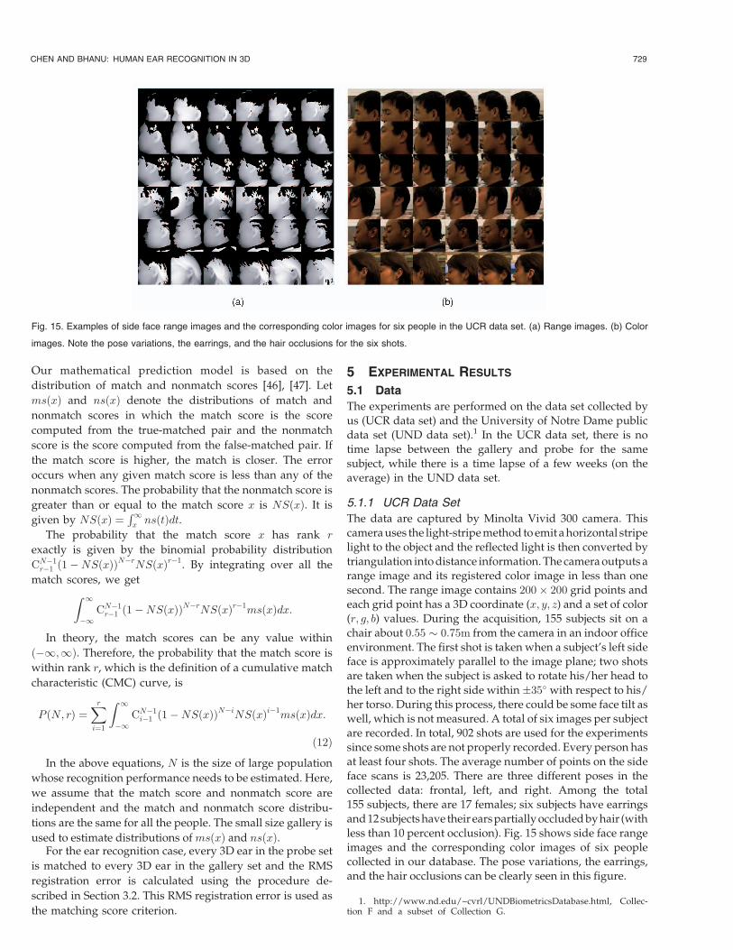
less than 10 percent occlusion). Fig. 15 shows side face rangeimages and the corresponding color images of six peoplecollected in our database. The pose variations, the earrings,and the hair occlusions can be clearly seen in this figure.


Fig. 15. Examples of side face range images and the corresponding color images for six people in the UCR data set. (a) Range images. (b) Color

images. Note the pose variations, the earrings, and the hair occlusions for the six shots.

1. http://www.nd.edu/~cvrl/UNDBiometricsDatabase.html, Collec-tion F and a subset of Collection G.

5.1.2 UND Data Set

The data are acquired with a Minolta Vivid 910 camera. Thecamera outputs a 480� 640 range image and its registeredcolor image of the same size. In Collection F, there are302 subjects with 302 time-lapse gallery-probe pairs. Fig. 16shows side face range images and the corresponding colorimages of two people from this collection. Collection Gcontains 415 subjects in which 302 subjects are from theCollection F. The most important part of Collection G is thatit has 24 subjects with images taken at four different viewpoints. We perform experiments only on these 24 subjects andnot the entire Collection G because Collection G becameavailable only very recently and it contains the entireCollection F. In this paper, we report the results on the entireCollection F. The identification results (rank-1 recognitionrate) by Yan and Bowyer are similar on Collection F(98.7 percent) and Collection G (97.6 percent) [9], [13].Therefore, we report and compare the rank-1 identificationperformance of algorithms on a subset of Collection G withpose variations.

5.2 Ear Detection Results

5.2.1 Ear Detection on UCR Data Set

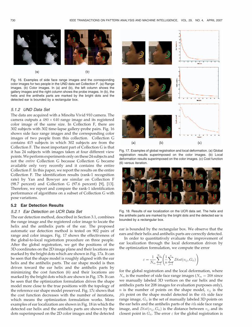
The ear detection method, described in Section 3.1, combinesthe range image and the registered color image to locate thehelix and the antihelix parts of the ear. The proposedautomatic ear detection method is tested on 902 pairs ofrange and color images. Fig. 17 shows the effectiveness ofthe global-to-local registration procedure on three people.After the global registration, we get the positions of the3D coordinates on the 2D image plane and their locations aremarked by the bright dots which are shown in Fig. 17a. It canbe seen that the shape model is roughly aligned with the earhelix and the antihelix parts. The ear shape model is thendriven toward the ear helix and the antihelix parts byminimizing the cost function (6) and their locations aremarked by the bright dots which are shown in Fig. 17b. It canbe seen that the optimization formulation drives the shapemodel more close to the true positions with the topology ofthe reference ear shape model preserved. Fig. 17c shows thatthe cost function decreases with the number of iterations,which means the optimization formulation works. Moreexamples of ear localization are shown in Fig. 18 in which thedetected ear helix and the antihelix parts are shown by thedots superimposed on the 2D color images and the detected

ear is bounded by the rectangular box. We observe that theears and their helix and antihelix parts are correctly detected.

In order to quantitatively evaluate the improvement ofear localization through the local deformation driven bythe optimization formulation, we compute the error

" ¼ 1

Nm

XNm

i¼1

1

n

Xnj¼1

Distðvij; GtiÞ !

for the global registration and the local deformation, whereNm is the number of side face range images (Nm ¼ 208 sincewe manually labeled 3D vertices on the ear helix and theantihelix parts for 208 images for evaluation purposes only),n is the number of points on the shape model, vij is thejth point on the shape model detected in the ith side facerange image, Gti is the set of manually labeled 3D points onthe ear helix and the antihelix parts of the ith side face rangeimage, and Distðvij; GtiÞ is the distance between vij and itsclosest point in Gti. The error " for the global registration is


Fig. 16. Examples of side face range images and the correspondingcolor images for two people in the UND data set Collection F. (a) Rangeimages. (b) Color images. In (a) and (b), the left column shows thegallery images and the right column shows the probe images. In (b), thehelix and the antihelix parts are marked by the bright dots and thedetected ear is bounded by a rectangular box.

Fig. 17. Examples of global registration and local deformation. (a) Global

registration results superimposed on the color images. (b) Local

deformation results superimposed on the color images. (c) Cost function

(6) versus iteration.

Fig. 18. Results of ear localization on the UCR data set. The helix and

the antihelix parts are marked by the bright dots and the detected ear is

bounded by a rectangular box.

5.4 mm; the error " after the local deformation is 3.7 mm.Thus, the local deformation driven by the optimizationformulation really improves the localization accuracy. Theproposed global-to-local procedure with the optimizationformulation can be applied to handle the nonrigid shaperegistration. This is shown in the supplemental material(Section A) associated with this paper [25], which can befound at http://computer.org/tpami/archives.htm.

Fig. 19 shows the extracted ears from the side face rangeimages in Fig. 15. The average number of points on the earsextracted from 902 side face images is 2,797. The ear detectiontakes about 9.48 s with Matlab implementation on a 2.4 GCeleron CPU. If the reference ear shape model is aligned withthe ear helix and the antihelix parts in a side face range image,we classify it as a positive detection; otherwise a falsedetection. On the 902 side face range images, we achieve99.3 percent correct detection rate (896 out of 902).

5.2.2 Ear Detection on UND Data Set

Without changing the parameters of the ear detectionalgorithm on the UCR data set, the proposed automatic eardetection method is tested on 700 (302� 2þ 24� 4 ¼ 700)pairs of range and color images of the UND data set(Collections F and a subset of Collection G). We achieve87.71 percent correct detection rate (614 out of 700). Theaverage number of points (on 700 images) on the ears is 6,348.Fig. 16b shows the extracted ears from the side face rangeimages in which the ear helix and the antihelix are markedby bright points and the extracted ear is bounded by arectangular box.

5.3 Ear Recognition Results

In order to evaluate and compare the matching performanceon the selected data sets, all the ears are correctly extracted. Inthese limited cases where the ears are not successfullydetected in an automated manner, they are correctlyextracted by human interaction. Note that we use LSP andhelix/antihelix representations separately for the matching.In the UCR data set, there are 155 subjects with 902 images.

The data are split into a gallery set and a probe set. Each sethas 155 subjects and every subject in the probe set has aninstance in the gallery set. In order to evaluate the proposedsurface matching schemes, we perform experiments undertwo scenarios: 1) One frontal ear of a subject is in the galleryset and another frontal ear of the same subject is in the probeset and 2) two frontal ears of a subject are in the gallery set andthe rest of the ear images of the same subject are in the probeset. These two scenarios are denoted as ES1 and ES2,respectively. ES1 is used for testing the performance of thesystem to recognize ears with the same pose; ES2 is used fortesting the performance of the system to recognize ears withpose variations. In the UND data set Collection F, there are302 subjects and each subject has two images. The gallery sethas 302 images and the probe set has the corresponding302 images. The experimental results on the UND data setCollection F are obtained using the same parameters of the earrecognition algorithm as those used on the UCR data set. Notethat the resolution of the sensors for the UCR and UND datasets are different. We anticipate improvement in performanceby fine tuning the parameters on the UND data set. However,these experiments are not performed since we wanted tokeep the algorithm parameters fixed across data sets.

5.3.1 Identification Performance

Every probe is matched to every 3D ear in the gallery set andthe RMS registration error is calculated using the proceduredescribed in Section 3.2. The subject in the gallery set with theminimum error is declared as the recognized person in theprobe image. The identification performance is evaluated bythe cumulative match characteristics (CMC), which describes“is the right answer in the top rank-r matches?” Table 5 showsthe rank-r recognition rates for the UCR data set and the UNDdata set Collection F using the ear helix/antihelix and the LSPrepresentations. In Table 5, the numbers of images in thegallery and the probe sets are listed in the parenthesisfollowing the name of the data set. Using the ear helix/antihelix representation, we achieve 96.77 percent rank-1recognition rate (150 out of 155) on the UCR data setES1 and96.36 percent rank-1 recognition rate (291 out of 302) on theUND data set Collection F. As expected, the system performsbetter on ES1 with the same pose and the performancedegrades slightly on ES2 with pose variations. The perfor-mance of the system using the LSP representation is betterthan the helix/antihelix representation on the UND data setbut a little lower on the UCR data set. We observe that,without retuning the parameters of the proposed algorithm,we still achieved good recognition performance on the UNDdata set, which has several weeks of time lapse between thegallery and the probe. For the LSP representation, the averagetime to match a pair of ears, which includes computation of


Fig. 19. Examples of extracted ears (from left to right and top to bottom)

in the side face range images shown in Fig. 15.

TABLE 5Cumulative Matching Performance on the UCR Data Set and the UND Data Set Collection F

LSPs and surface matching, is about 3.7 seconds with C++implementation on a Linux machine with a AMD Opteron1.8 GHz processor. For the helix/antihelix representation, theaverage time to match a pair of ears is about 1.1 seconds withC++ implementation on the same platform.

Fig. 20 shows three examples of the correctly recognizedgallery-probe ear pairs with a large pose variation using theear helix/antihelix representation. Fig. 20a shows the sideface color images of the gallery and the probe alternately,Fig. 20b shows the range images of the ears that areautomatically extracted and Fig. 20c shows the gallery earrepresented by the mesh overlaid on the textured 3D probeear images. We observe that the cases with a large posevariation are correctly handled.

We show four special cases of correctly recognizinggallery-probe ear pairs using the LSP representation inFig. 21. In this figure, each probe ear is rendered as a textured3D surface and each gallery ear is displayed as a mesh. Inorder to examine the results visually, we display theprealigned gallery ear and the probe ear in the same image(Fig. 21b) and also the postaligned (transformed) gallery andthe probe ear in the same image (Fig. 21c). From Fig. 21, we

observe that the ear recognition system can handle partialocclusion. Twelve more examples of correctly recognizedgallery-probe ear pairs (using both the helix/antihelix andthe LSP representations) are shown in the supplementalmaterial (Section C) that accompanies this paper [25], whichcan be found at http://computer.org/tpami/archives.htm.

During the recognition, some errors are made and the fourerror cases are illustrated in Fig. 22. Figs. 22a and 22b show thecolor images of two visually similar probe and gallery earsthat belong to different subjects; Fig. 22c shows the truegallery ear overlaid on the textured 3D probe ear afterregistration; Fig. 22d shows the falsely recognized gallery earoverlaid on the textured 3D probe ear after alignment. InFig. 22d, the root mean square error for the falsely recognizedear is smaller than the error for the correct ear in Fig. 22c. Inthis figure, we obtain good alignment between the gallery andprobe ears from different people since these ears are quitesimilar in 3D.

5.3.2 Verification Performance

The verification performance of the proposed system isevaluated in terms of the two popular methods, the receiveroperating characteristic (ROC) curve and the equal errorrate (EER). The ROC curve is the plot of the genuineacceptance rate (GAR) versus the corresponding falseacceptance rate (FAR). GAR is defined as the percentageof the occurrences where an authorized user is correctlyaccepted by the system, while FAR is defined as the


Fig. 20. UCR data set: Three cases of the correctly recognized gallery-probe ear pairs using the ear helix/antihelix representation with a largepose variation. (a) Side face color images. (b) Range images of thedetected ears. In columns (a) and (b), the gallery image is shown firstand the probe image is shown second. (c) The probe ear with thecorresponding gallery ear after alignment. The gallery ear representedby the mesh is overlaid on the textured 3D probe ear. The units of X, Y,and Z are millimeters (mm). In Case 1, the rotation angle is 33:5� and theaxis is ½0:0099; 0:9969; 0:0778�T . In Case 2, the rotation angle is �33:5�

and the axis is ½�0:1162; 0:9932; 0:0044�T . In Case 3, the rotation angle is32:9� and the axis is ½0:0002; 0:9998; 0:0197�T .

Fig. 21. UCR data set: Four examples of the correctly recognizedgallery-probe pairs using the LSP representation. Two ears haveearrings and the other two ears are partially occluded by the hair.Images in (a) show color images of ears. Images in (b) and (c) show theprobe ear with the corresponding gallery ear before the alignment andafter the alignment, respectively. The gallery ears represented by themesh are overlaid on the textured 3D probe ears. The units of X, Y, andZ are millimeters (mm).

percentage of the occurrences where a nonauthorized useris falsely accepted by the system. The EER, which, indicatesthe rate at which the false rejection rate (FRR ¼ 1�GAR)and the false acceptance rate are equal, is a thresholdindependent performance measure.

During the verification, the RMS distance is computedfrom matching the gallery ears to the probe ears and it is thencompared to a threshold to determine if the probe is anauthorized user or an imposter. By varying the threshold,FAR and GAR values are computed and plotted in Fig. 23.

Fig. 23a shows the ROC curves on the UCR and the UND dataset Collection F using the ear helix/antihelix representationfor surface matching; Fig. 23b shows the ROC curves on theUCR and the UND data set Collection F using the LSPrepresentation for surface matching. As expected, the systemperforms better on ES1 than on ES2 using the ear helix/antihelix and the LSP representations. We obtain the bestperformance with a 0.023 EER on the UND data set using theLSP representation. It is clearly seen that, without retuningthe parameters of the proposed algorithms, we achieved goodverification performance on the UND data set.

Based on the ROC curve, we can select a threshold whichsatisfies the user’s requirement for the false alarm rate orfalse rejection rate. This threshold can be used to reject theunauthorized users.

5.3.3 Evaluation of the Verification Performance

We discuss and evaluate the accuracy of the ear verificationsystem following the method in [16], [48], [49]. As describedin Section 5.1, the UCR data set has 155 subjects. There are155 probes providing 155 user claims and 23,870 (155� 154)imposter claims for the UCR data set ES1. For the UCR dataset ES2, there are 592 probes providing 592 user claims and91,168 (592� 154) imposter claims. The UND data setCollection F has 302 subjects. There are 302 pairs of imagesproviding 302 user claims and 90,902 (302� 301) imposterclaims.

We calculate the number of user claims and imposterclaims that gives statistically significant results. Let ��denote the �-percentile of the standard Gaussian distributionwith zero mean and unit variance. Since the verificationtests can be thought of as Bernoulli trials, we can assert that,with confidence � ¼ 1� �, the minimum number of userclaims which ensures that the expected value of FRR (pFR)and the empirical value (bpFR) are related by jpFR � bpFRj � is given by

�C ¼� ��=2

�2pFRð1� pFRÞ: ð13Þ

The number �I of the imposter claims [49] which issufficient to ensure that the expected value of FAR (pFA)and the empirical value (bpFA) are related by jpFA � bpFAj � is given by:


Fig. 22. UCR data set: Four cases of incorrectly recognized gallery-probe pairs using the ear helix/antihelix representation. Each row showsone case. The gallery ears represented by the mesh are overlaid on thetextured 3D probe ears. The units of X, Y, and Z are millimeters (mm).(a) Color images of the probe ears. (b) Color images of falselyrecognized gallery ears. (c) True gallery ears after alignment areoverlaid on the textured 3D probe ears. (d) The falsely recognizedgallery ears after alignment are overlaid on the textured 3D probe ears.Note that, for the incorrect matches, the gallery ears (d) achieve asmaller value of RMS error than the gallery ears in (c).

Fig. 23. UCR data set and UND data set Collection F: Verification performance as an ROC curve. (a) ROC curves on the UCR data set ES1, ES2,

and the UND data set using the ear helix/antihelix representation. (b) ROC curves on the UCR data set ES1, ES2 and the UND data set using the

LSP representation.

�I ¼� ��=2

0

�2

poð1� poÞ; 0 ¼

k; ð1� poÞk ¼ 1� pFA; ð14Þ

where po is the probability that one imposter is falselyaccepted as an authorized user and k is the number ofimposter claims (k ¼ 154 for the UCR data set and k ¼ 301for the UND data set Collection F). By setting the desiredEER, � and , we can compute �C and �I . For the UCR dataset ES1, we find �C ¼ 149 and �I ¼ 24; 759 with EER ¼ 5%,� ¼ 95%, and ¼ 3:5%. For the UCR data set ES2, we find�C ¼ 456 and �I ¼ 75; 826 with EER ¼ 5%, � ¼ 95%, and ¼ 2%. For the UND data set Collection F, we find �C ¼ 292and �I ¼ 94; 874 with EER ¼ 5%, � ¼ 95%, and ¼ 2:5%.Note that the order of magnitude of these numbers are thesame as those provided by the test scenarios. The values of on the UCR data set ES2 ( ¼ 2%) and the UND data setCollection F ( ¼ 2:5%) are smaller than the value on theUCR data set ES1 ( ¼ 3:5%) since the UCR data set ES2

and the UND data set Collection F are larger in size than thesize of the UCR data set ES1.

5.3.4 Comparison between Chen and Bhanu’s

Approach and Yan and Bowyer’s Approach

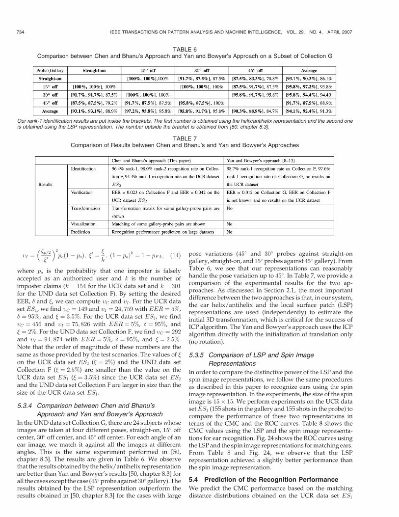
In the UND data set Collection G, there are 24 subjects whoseimages are taken at four different poses, straight-on, 15� offcenter, 30� off center, and 45� off center. For each angle of anear image, we match it against all the images at differentangles. This is the same experiment performed in [50,chapter 8.3]. The results are given in Table 6. We observethat the results obtained by the helix/antihelix representationare better than Yan and Bowyer’s results [50, chapter 8.3] forall the cases except the case (45� probe against 30� gallery). Theresults obtained by the LSP representation outperform theresults obtained in [50, chapter 8.3] for the cases with large

pose variations (45� and 30� probes against straight-ongallery, straight-on, and 15� probes against 45� gallery). FromTable 6, we see that our representations can reasonablyhandle the pose variation up to 45�. In Table 7, we provide acomparison of the experimental results for the two ap-proaches. As discussed in Section 2.1, the most importantdifference between the two approaches is that, in our system,the ear helix/antihelix and the local surface patch (LSP)representations are used (independently) to estimate theinitial 3D transformation, which is critical for the success ofICP algorithm. The Yan and Bowyer’s approach uses the ICPalgorithm directly with the initialization of translation only(no rotation).

5.3.5 Comparison of LSP and Spin Image

Representations

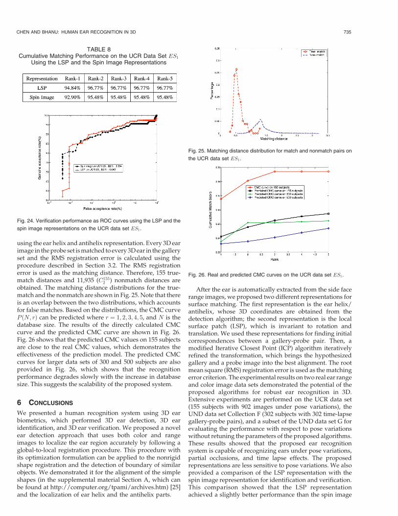
In order to compare the distinctive power of the LSP and thespin image representations, we follow the same proceduresas described in this paper to recognize ears using the spinimage representation. In the experiments, the size of the spinimage is 15� 15. We perform experiments on the UCR datasetES1 (155 shots in the gallery and 155 shots in the probe) tocompare the performance of these two representations interms of the CMC and the ROC curves. Table 8 shows theCMC values using the LSP and the spin image representa-tions for ear recognition. Fig. 24 shows the ROC curves usingthe LSP and the spin image representations for matching ears.From Table 8 and Fig. 24, we observe that the LSPrepresentation achieved a slightly better performance thanthe spin image representation.

5.4 Prediction of the Recognition Performance

We predict the CMC performance based on the matchingdistance distributions obtained on the UCR data set ES1


TABLE 6Comparison between Chen and Bhanu’s Approach and Yan and Bowyer’s Approach on a Subset of Collection G

Our rank-1 identification results are put inside the brackets. The first number is obtained using the helix/antihelix representation and the second oneis obtained using the LSP representation. The number outside the bracket is obtained from [50, chapter 8.3].

TABLE 7Comparison of Results between Chen and Bhanu’s and Yan and Bowyer’s Approaches

using the ear helix and antihelix representation. Every 3D earimage in the probe set is matched to every 3D ear in the galleryset and the RMS registration error is calculated using theprocedure described in Section 3.2. The RMS registrationerror is used as the matching distance. Therefore, 155 true-match distances and 11,935 (C155

2 ) nonmatch distances areobtained. The matching distance distributions for the true-match and the nonmatch are shown in Fig. 25. Note that thereis an overlap between the two distributions, which accountsfor false matches. Based on the distributions, the CMC curveP ðN; rÞ can be predicted where r ¼ 1; 2; 3; 4; 5, and N is thedatabase size. The results of the directly calculated CMCcurve and the predicted CMC curve are shown in Fig. 26.Fig. 26 shows that the predicted CMC values on 155 subjectsare close to the real CMC values, which demonstrates theeffectiveness of the prediction model. The predicted CMCcurves for larger data sets of 300 and 500 subjects are alsoprovided in Fig. 26, which shows that the recognitionperformance degrades slowly with the increase in databasesize. This suggests the scalability of the proposed system.

6 CONCLUSIONS

We presented a human recognition system using 3D earbiometrics, which performed 3D ear detection, 3D earidentification, and 3D ear verification. We proposed a novelear detection approach that uses both color and rangeimages to localize the ear region accurately by following aglobal-to-local registration procedure. This procedure withits optimization formulation can be applied to the nonrigidshape registration and the detection of boundary of similarobjects. We demonstrated it for the alignment of the simpleshapes (in the supplemental material Section A, which canbe found at http://computer.org/tpami/archives.htm) [25]and the localization of ear helix and the antihelix parts.

After the ear is automatically extracted from the side facerange images, we proposed two different representations forsurface matching. The first representation is the ear helix/antihelix, whose 3D coordinates are obtained from thedetection algorithm; the second representation is the localsurface patch (LSP), which is invariant to rotation andtranslation. We used these representations for finding initialcorrespondences between a gallery-probe pair. Then, amodified Iterative Closest Point (ICP) algorithm iterativelyrefined the transformation, which brings the hypothesizedgallery and a probe image into the best alignment. The rootmean square (RMS) registration error is used as the matchingerror criterion. The experimental results on two real ear rangeand color image data sets demonstrated the potential of theproposed algorithms for robust ear recognition in 3D.Extensive experiments are performed on the UCR data set(155 subjects with 902 images under pose variations), theUND data set Collection F (302 subjects with 302 time-lapsegallery-probe pairs), and a subset of the UND data set G forevaluating the performance with respect to pose variationswithout retuning the parameters of the proposed algorithms.These results showed that the proposed ear recognitionsystem is capable of recognizing ears under pose variations,partial occlusions, and time lapse effects. The proposedrepresentations are less sensitive to pose variations. We alsoprovided a comparison of the LSP representation with thespin image representation for identification and verification.This comparison showed that the LSP representationachieved a slightly better performance than the spin image


Fig. 24. Verification performance as ROC curves using the LSP and the

spin image representations on the UCR data set ES1.

Fig. 25. Matching distance distribution for match and nonmatch pairs on

the UCR data set ES1.

TABLE 8Cumulative Matching Performance on the UCR Data Set ES1

Using the LSP and the Spin Image Representations

Fig. 26. Real and predicted CMC curves on the UCR data set ES1.

representation. Furthermore, the performance predictionmodel showed the scalability of the proposed system withincreased database size.

Our experimental results show that ear biometrics has thepotential to be used in the real-world applications to identify/authenticate humans by their ears. It can be used in both thelow and high security applications and in combination withother biometrics such as face. With the decreasing cost (fewthousand dollars) and size of a 3D scanner and the increasedperformance, we believe that 3D ear biometrics will be highlyuseful in many real-world applications in the future.

ACKNOWLEDGMENTS

The authors would like to thank the computer visionresearch laboratory at the University of Notre Dame forproviding their public biometrics database Collections Fand G that are used in this paper. The authors would like tothank Dr. Yan and Dr. Bowyer for providing theirpublications and some useful discussions.

REFERENCES

[1] BIOMETRICS: Personal Identification in Network Society, A. Jain et al.,eds. Kluwer Academic, 1999.

[2] A. Iannarelli, Ear Identification. Paramont Publishing, 1989.[3] M. Burge and W. Burger, “Ear Biometrics in Computer Vision,”

Proc. Int’l Conf. Pattern Recognition, vol. 2, pp. 822-826, 2000.[4] D. Hurley, M. Nixon, and J. Carter, “Force Field Feature

Extraction for Ear Biometrics,” Computer Vision and Image Under-standing, vol. 98, no. 3, pp. 491-512, 2005.

[5] K. Chang, K.W. Bowyer, S. Sarkar, and B. Victor, “Comparisonand Combination of Ear and Face Images in Appearance-BasedBiometrics,” IEEE Trans. Pattern Analysis and Machine Intelligence,vol. 25, no. 9, pp. 1160-1165, Sept. 2003.

[6] B. Bhanu and H. Chen, “Human Ear Recognition in 3D,” Proc.Workshop Multimodal User Authentication, pp. 91-98, 2003.

[7] H. Chen and B. Bhanu, “Contour Matching for 3D Ear Recogni-tion,” Proc. Seventh IEEE Workshop Application of Computer Vision,vol. 1, pp. 123-128, 2005.

[8] P. Yan and K.W. Bowyer, “Multi-Biometrics 2D and 3D EarRecognition,” Proc. Audio and Video-Based Biometric Person Authen-tication, pp. 503-512, 2005.

[9] P. Yan and K.W. Bowyer, “Empirical Evaluation of Advanced EarBiometrics,” Proc. IEEE Conf. Computer Vision and Pattern Recogni-tion Workshop Empirical Evaluation Methods in Computer Vision, 2005.

[10] P. Yan and K.W. Bowyer, “Ear Biometrics Using 2D and 3DImages,” Proc. IEEE Conf. Computer Vision and Pattern RecognitionWorkshop Advanced 3D Imaging for Safety and Security, 2005.

[11] P. Yan and K.W. Bowyer, “ICP-Based Approaches for 3D EarRecognition,” Proc. SPIE Conf. Biometric Technology for HumanIdentification, pp. 282-291, 2005.

[12] P. Yan and K.W. Bowyer, “A Fast Algorithm for ICP-Based 3DShape Biometrics,” Proc. IEEE Workshop Automatic IdentificationAdvanced Technologies, pp. 213-218, 2005.

[13] P. Yan and K.W. Bowyer, “An Automatic 3D Ear RecognitionSystem,” Proc. Third Int’l Symp. 3D Data Processing, Visualization,and Transmission, pp. 213-218, 2006.

[14] J.C. Lee and E. Milios, “Matching Range Images of Human Faces,”Proc. Int’l Conf. Computer Vision, pp. 722-726, 1990.

[15] G.G. Gordon, “Face Recognition Based on Depth and CurvatureFeatures,” Proc. IEEE Conf. Computer Vision and Pattern Recognition,pp. 808-810, 1992.

[16] F. Tsalakanidou, S. Malasiotis, and M.G. Strintzis, “Face Localiza-tion and Authentication Using Color and Depth Images,” IEEETrans. Image Processing, vol. 14, no. 2, pp. 152-168, 2005.

[17] C.S. Chua, F. Han, and Y. Ho, “3D Human Face Recognition UsingPoint Signatures,” Proc. Int’l Conf. Automatic Face and GestureRecognition, pp. 233-238, 2000.

[18] A. Bronstein, M. Bronstein, and R. Kimmel, “Expression-Invariant3D Face Recognition,” Proc. Audio and Video-Based Biometric PersonAuthentication, pp. 62-70, 2003.

[19] K. Chang, K.W. Bowyer, and P. Flynn, “An Evaluation ofMultimodal 2D+3D Face Biometrics,” IEEE Trans. Pattern Analysisand Machine Intelligence, vol. 27, no. 4, pp. 619-624, Apr. 2005.

[20] X. Lu and A.K. Jain, “Integrating Range and Texture Informationfor 3D Face Recognition,” Proc. Seventh IEEE Workshop Applicationof Computer Vision, vol. 1, pp. 156-163, 2005.

[21] M.J. Jones and J.M. Rehg, “Statistical Color Models withApplication to Skin Detection,” Int’l J. Computer Vision, vol. 46,no. 1, pp. 81-96, 2002.

[22] T.F. Cootes, D. Cooper, C.J. Taylor, and J. Graham, “Active ShapeModels—Their Training and Application,” Computer Vision andImage Understanding, vol. 61, no. 1, pp. 38-59, 1995.

[23] C.S. Chen, Y.P. Hung, and J.B. Cheng, “RANSAC-Based DARCES:A New Approach to Fast Automatic Registration of PartiallyOverlapping Range Images,” IEEE Trans. Pattern Analysis andMachine Intelligence, vol. 21, no. 11, pp. 1229-1234, Nov. 1999.

[24] F.L. Bookstein, “Principal Warps: Thin-Plate Splines and theDecomposition of Deformations,” IEEE Trans. Pattern Analysis andMachine Intelligence, vol. 11, no. 6, pp. 567-585, June 1989.

[25] H. Chen and B. Bhanu, “Supplemental Material to Accompany‘Human Ear Recognition in 3D’,” http://computer.org/tpami/archives.htm, 2007.

[26] C. Boehnen and T. Russ, “A Fast Multi-Modal Approach to FacialFeature Detection,” Proc. Seventh IEEE Workshops Application ofComputer Vision, vol. 1, pp. 135-142, 2005.

[27] X. Lu, D. Colbry, and A.K. Jain, “Three-Dimensional Model BasedFace Recognition,” Proc. Int’l Conf. Pattern Recognition, vol. 1,pp. 362-366, 2004.

[28] S.H. Kim, N.K. Kim, S.C. Ahn, and H.G. Kim, “Object OrientedFace Detection Using Range and Color Information,” Proc. Int’lConf. Face and Gesture Recognition, pp. 76-81, 1998.

[29] H. Chen and B. Bhanu, “Human Ear Detection from Side FaceRange Images,” Proc. Int’l Conf. Pattern Recognition, vol. 3, pp. 574-577, 2004.

[30] H. Chen and B. Bhanu, “Shape Model-Based 3D Ear Detectionfrom Side Face Range Images,” Proc. IEEE Conf. Computer Visionand Pattern Recognition Workshop Advanced 3D Imaging for Safetyand Security, 2005.

[31] P. Besl and N.D. Mckay, “A Method of Registration of 3D Shapes,”IEEE Trans. Pattern Analysis and Machine Intelligence, vol. 14, no. 2,pp. 239-256, Feb. 1992.

[32] Y. Chen and G. Medioni, “Object Modelling by Registration ofMultiple Range Images,” Image and Vision Computing, vol. 10,no. 3, pp. 145-155, 1992.

[33] Z. Zhang, “Iterative Point Matching for Registration of Free-FormCurves and Surfaces,” Int’l J. Computer Vision, vol. 13, no. 2,pp. 119-152, 1994.

[34] S. Rusinkiewicz and M. Levoy, “Efficient Variants of the ICPAlgorithm,” Proc. Int’l Conf. 3-D Digital Imaging and Modeling,pp. 145-152, 2001.

[35] H. Chui and A. Rangaraian, “A New Algorithm for Non-RigidPoint Matching,” Proc. IEEE Conf. Computer Vision and PatternRecognition, vol. 2, pp. 44-51, 2000.

[36] S. Wang, T. Kubota, and T. Richardson, “Shape Correspondencethrough Landmark Sliding,” Proc. IEEE Conf. Computer Vision andPattern Recognition, vol. 1, pp. 143-150, 2004.

[37] J. Lim and M.H. Yang, “A Direct Method for Modeling NonRigidMotion with Thin Plate Spline,” Proc. IEEE Conf. Computer Visionand Pattern Recognition, vol. 1, pp. 196-202, 2005.

[38] M. Kass, A. Witkin, and D. Terzopoulos, “Snakes: Active ContourModels,” Int’l J. Computer Vision, vol. 1, no. 14, pp. 321-331, 1988.

[39] B. Horn, “Close-Form Solution of Absolute Orientation Using UnitQuaternions,” J. Optical Soc. Am., vol. 4, no. 4, pp. 629-642, 1987.

[40] R.J. Campbell and P.J. Flynn, “A Survey of Free-Form ObjectRepresentation and Recognition Techniques,” Computer Vision andImage Image Understanding, vol. 81, pp. 166-210, 2001.

[41] P. Flynn and A. Jain, “On Reliable Curvature Estimation,” Proc.IEEE Conf. Computer Vision and Pattern Recognition, pp. 110-116,1989.

[42] C. Dorai and A. Jain, “COSMOS-A Representation Scheme for 3DFree-Form Objects,” IEEE Trans. Pattern Analysis and MachineIntelligence, vol. 19, no. 10, pp. 1115-1130, Oct. 1997.

[43] J.J. Koenderink and A.V. Doorn, “Surface Shape and CurvatureScales,” Image Vision Computing, vol. 10, no. 8, pp. 557-565, 1992.

[44] A. Johnson and M. Hebert, “Using Spin Images for Efficient ObjectRecognition in Cluttered 3D Scenes,” IEEE Trans. Pattern Analysisand Machine Intelligence, vol. 21, no. 5, pp. 433-449, May 1999.


[45] B. Schiele and J. Crowley, “Recognition without CorrespondenceUsing Multidimensional Receptive Field Histograms,” Int’l J.Computer Vision, vol. 36, no. 1, pp. 31-50, 2000.

[46] B. Bhanu, R. Wang, and X. Tan, “Predicting Fingerprint Recogni-tion Performance from a Small Gallery,” Pattern RecognitionLetters, vol. 28, pp. 40-48, 2007.

[47] H. Chen, B. Bhanu, and R. Wang, “Performance Evaluation andPrediction for 3D Ear Recognition,” Proc. Conf. Audio and Video-Based Biometric Person Authentication, pp. 748-757, 2005.

[48] C. Kotropoulos, A. Tefas, and I. Pitas, “Frontal Face Authentica-tion Using Discriminating Grids with Morphological FeatureVectors,” IEEE Trans. Multimedia, vol. 2, no. 1, pp. 14-26, Jan.-Mar.2000.

[49] W. Shen, M. Surette, and R. Khanna, “Evaluation of AutomatedBiometric-Based Identification and Verification Systems,” Proc.IEEE, vol. 85, no. 9, pp. 1464-1478, 1997.

[50] P. Yan, “Ear Biometrics in Human Identification,” PhD dissertation,Dept. of Computer Science and Eng., Univ. of Notre Dame, 2006.

Hui Chen received the MS and BS degree incontrol theory and applications from the Uni-versity of Science and Technology, Beijing,China, in 1999 and 1996, respectively, and thePhD degree in electrical engineering from theUniversity of California at Riverside in 2006.He worked as a software engineer at theChinese Academy of Sciences, Beijing, China,during 1999-2001. He also worked as an internat Siemens Medical Solutions, Malvern, Penn-

sylvania, during the summer of 2005. His research interests are3D object detection, tracking, and recognition, medical imageprocessing, 3D biometrics, shape registration, and range imageanalysis. He is a student member of the IEEE.

Bir Bhanu received the SM and EE degrees inelectrical engineering and computer sciencefrom the Massachusetts Institute of Technology,Cambridge, the PhD degree in electrical en-gineering from the Image Processing Institute,University of Southern California, Los Angeles,and the MBA degree from the University ofCalifornia, Irvine. He was the founding professorof electrical engineering and served as its firstchair at the University of California at Riverside

(UCR). He has been the Cooperative Professor of Computer Scienceand Engineering and the director of the Visualization and IntelligentSystems Laboratory (VISLab) since 1991. Currently, he also serves asthe founding director of an interdisciplinary Center for Research inIntelligent Systems (CRIS) at UCR. Previously, he was a SeniorHoneywell Fellow at Honeywell Inc., Minneapolis, Minnesota. He hasbeen on the faculty of the Department of Computer Science at theUniversity of Utah, Salt Lake City, and has worked at Ford Aerospaceand Communications Corporation, California, INRIA-France, and IBMSan Jose Research Laboratory, California. He has been the principalinvestigator of various programs for the NSF, DARPA, NASA, AFOSR,ARO, and other agencies and industries in the areas of video networks,video understanding, learning and vision, image understanding, patternrecognition, target recognition, biometrics, navigation, image databases,and machine vision applications. He is the coauthor of the booksComputational Learning for Adaptive Computer Vision (Springer-Verlag,2007), Evolutionary Synthesis of Pattern Recognition Systems (Spring-er-Verlag, 2005), Computational Algorithms for Fingerprint Recognition(Kluwer, 2004), Genetic Learning for Adaptive Image Segmentation(Kluwer, 1994), and Qualitative Motion Understanding (Kluwer, 1992),and the coeditor of the book Computer Vision Beyond the VisibleSpectrum (Springer-Verlag, 2004). He holds 11 US and internationalpatents and more than 250 reviewed technical publications in the areasof his interest. Dr. Bhanu has received two outstanding paper awardsfrom the Pattern Recognition Society and has received industrial anduniversity awards for research excellence, outstanding contributions,and team efforts. He has been on the editorial board of various journalsand has edited special issues of several IEEE transactions (TPAMI, IP,SMC-B, R&A, IFS) and other journals. He was general chair for the IEEEConference on Computer Vision and Pattern Recognition, IEEE Work-shops on Applications of Computer Vision, IEEE Workshops onLearning in Computer Vision and Pattern Recognition; chair for theDARPA Image Understanding Workshop, and program chair for theIEEE Workshops on Computer Vision Beyond the Visible Spectrum andMulti-Modal Biometrics. He is a fellow of the IEEE, the IEEE ComputerSociety, American Association for the Advancement of Science (AAAS),International Association of Pattern Recognition (IAPR), and theInternational Society for Optical Engineering (SPIE).

. For more information on this or any other computing topic,please visit our Digital Library at www.computer.org/publications/dlib.


718 ieee transactions on pattern analysis and … and... · propose a complete human recognition...

Documents