6TH INTERNATIONAL CONFERENCE ON ELECTROMECHANICAL AND POWER SYSTEMS October 4-6, 2007 - Chişinău, Rep.Moldova

26

SIMULATION OF A TEMPERATURE CONTROL SYSTEM WITH DISBRIBUTED PARAMETERS

Marius Constantin POPESCU, Anca PETRISOR

University of Craiova, Faculty of Electromechanical Engineering

Abstract −−−− In this paper is simulated, both numerical and on experimental model, a glass annealing system, usefully to study those phenomenon that appear to the control system implementation of the technological process for glass annealing.

Keywords: distributed parameters system, glass annealing.

1. INTRODUCTION

The manufacture process developed in the glass factory it doesn’t stop together with the forming or modeling of the glass products. After these stages some operations are required, the most important of them been the stress relieving through annealing. The annealing process consists of the glass products cooling according to a special annealing condition, having four stages [6]: heating of the glass articles up to the annealing or stress relieving temperature; stress relieving and maintaining of the articles to a temperature between the limits of the stress relieving interval; slow cooling of the glass in order not to get arisen new internal stresses in the product and quick cooling of the glass. Through the technical analysis of the glass products one can elaborate the

temperature profile that has to be maintained (figure1).

Figure 1: The shape of the temperature imposed in the glass annealing process nonlinear characteristic.

2. EXPERIMENTAL MODEL OF THE PRODUCTION SYSTEM

The heating furnace is like a four areas divided tunnel, each area representing one stage of the annealing process (figure 2).

Figure 2: Experimental model used for simulation of the glass annealing process.

S2S1 S3

V1 V2

Z I Z II Z III Z IV V3

B1 B2 B3

2 2 4 2(m)

27

3. THE STRUCTURE THE STRUCTURE OF ACQUISITION AND CONTROL SYSTEM

Processing the data from the process, respectively reading the temperature, is realized with an integrated sensor LM 35 DZ made by National Semiconductor. The electronic diagram for connecting the temperature sensor is presented in figure 3. The resistances dimensioning was made in such way that for T=100oC to obtain an output voltage u0=5V – maximum value of the analogical input voltage for the acquisition board.

Figure 3: Schema of temperature controller.

Figure 4: Configuration of the acquisition and control system.

The acquisition and control system is realized with a micro-controller board INTEL80C32 and has the structure from figure 4 [1], [3]. For implementing on the experimental model of the technological process, there have been realized several electronic diagrams, most relevant of them being [2], [5]: the supply source for the acquisition board (–5V); the supply source for the triac control board (±15V); the supply source for the differential control board and the analogical extension of the acquisition board (±15V); the differential control (figure 5); connecting of the triac (figure 6) and control of the triac (figure 7).

a)

b)

Figure 5: Differential control: a) electronic diagram; b) general view of the electronic card.

28

Figure 6: The triac connection: a) electronic diagram; b) general view of the electronic card.

Figure 7: The triac control: a) electronic diagram; b) general view of the electronic card.

4. IMPLEMENTATION OF THE REGULATION SYSTEM WITH DISTRIBUTED PARAMETERS

4.1. Calculation of the decoupling matrix

Temperature control systems are slow processes, described by time constants bigger than 10 s. The transfer functions for the fixed parts of the heating furnace areas are approximated as [7]:

sEE

E

kH (s) eT s 1

−τ= ⋅+

(1)

The fixed part of the heating furnace will be considered as a multivariable system with the inputs U1, U2, U3 and the outputs Y1, Y2, Y3, as in figure 8.

Figure 8: The structure of a multivariable system.

The transfer function of the fixed part it was considered as:

1

2

3

Y (s)Y (s)Y (s)

=F11

F12 F22

F23 F33

H (s) 0 0H (s) H (s) 0

0 H (s) H (s)

1

2

3

U (s)U (s)U (s)

(2)

29

It shall be calculated a decoupling matrix, attempting to decouple the input/output channels, in such way to

obtain an equivalent transfer function Hv(s).

Figure 9: Explanatory regarding channels decoupling.

Imposing a desired behaviour for Hv(s), meaning been at most of order II, it results:

C Fy(s) H(s) V(s) H (s) H (s) V(s)= ⋅ = ⋅ ⋅ ⇒

V C FH (s) H (s) H (s)= ⋅ (3)

Having the conditions HF(s)-estimated, HV(s)-imposed, results that HC(s) can be determinated by solving the equations system [4]:

11

22

33

H (s) 0 00 H (s) 00 0 H (s)

=

C11 C21 C31

C12 C22 C32

C13 C23 C33

H (s) H (s) H (s)H (s) H (s) H (s)H (s) H (s) H (s)

F11

F12 F22

F23 F33

H (s) 0 0H (s) H (s) 0

0 H (s) H (s)

(4)

The following values are obtained for the elements of the matrix HC:

HC=

11

F11

22 F12 22

F22 F11 F22

33 F12 F23 33 F23 33

F22 F11 F33 F22 F33

H o oH

H H H oH H H

H H H H H HH H H H H

⋅−

⋅ ⋅ ⋅ ⋅

− ⋅ ⋅

(5)

4.2. System identification

For the system identification, a program in Labwindows/CVI developing environment was realized. With this program, the computer will control the inputs U1, U2, U3, through the acquisition and control system. First area implementation is realized by the control Bec1=1L, Bec2=0L, Bec3=0L, the ventilator V1=0%; V2=0%; V3=0%;, that implements a control U1=100% for the heating process (figure 10).

Figure 10: OFF-line testing application of the acquisition and control system.

30

4.3. Implementation of the control system

Implementation of the control system is realized

through three controlling loops for the decoupling system.

Figure 11: Simulink program.

Figure 12: Multivariable system simulation using Simulink.

31

5. CONCLUSIONS

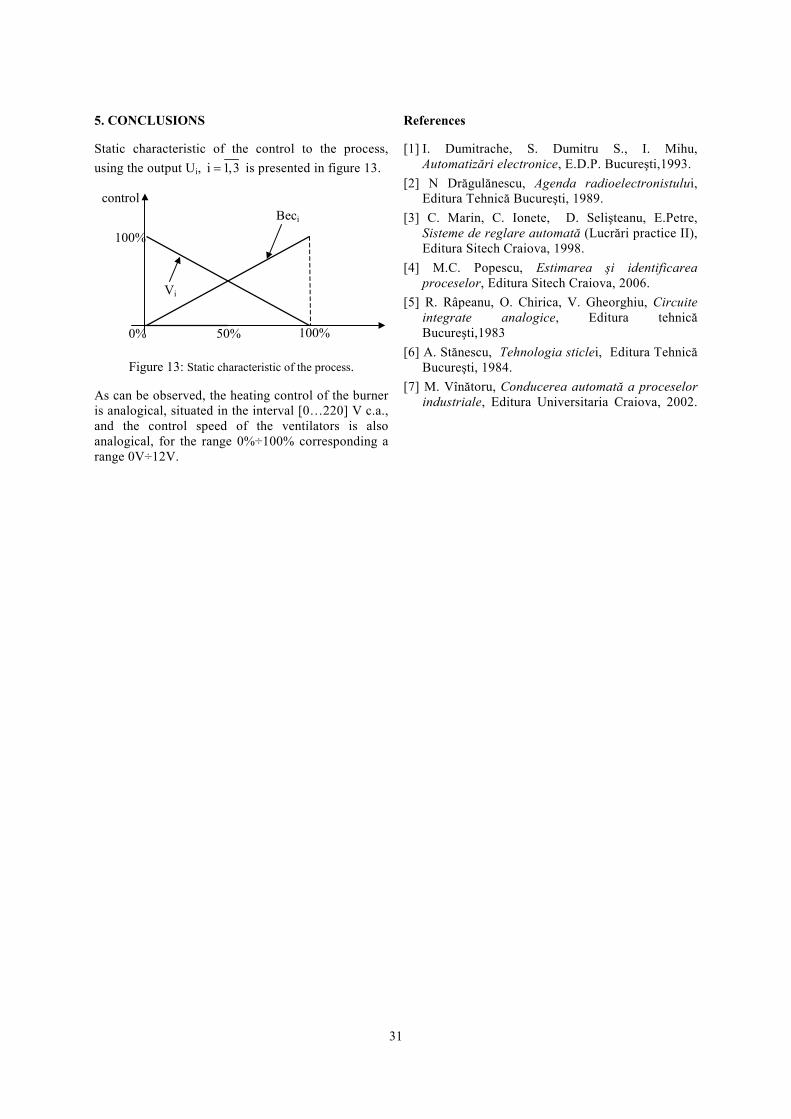
Static characteristic of the control to the process, using the output Ui, i 1,3= is presented in figure 13.

Figure 13: Static characteristic of the process.

As can be observed, the heating control of the burner is analogical, situated in the interval [0…220] V c.a., and the control speed of the ventilators is also analogical, for the range 0%÷100% corresponding a range 0V÷12V.

References

[1] I. Dumitrache, S. Dumitru S., I. Mihu, Automatizări electronice, E.D.P. Bucureşti,1993.

[2] N Drăgulănescu, Agenda radioelectronistului, Editura Tehnică Bucureşti, 1989.

[3] C. Marin, C. Ionete, D. Selişteanu, E.Petre, Sisteme de reglare automată (Lucrări practice II), Editura Sitech Craiova, 1998.

[4] M.C. Popescu, Estimarea şi identificarea proceselor, Editura Sitech Craiova, 2006.

[5] R. Râpeanu, O. Chirica, V. Gheorghiu, Circuite integrate analogice, Editura tehnicăBucureşti,1983

[6] A. Stănescu, Tehnologia sticlei, Editura TehnicăBucureşti, 1984.

[7] M. Vînătoru, Conducerea automată a proceselor industriale, Editura Universitaria Craiova, 2002.

100%0% 50%

Beci

Vi

100%

control