Underground Cable Parameter Estimation Using Time-Synchronized Event Data and

Line Energization Data

Hibourahima Camara, Jasvinder Blah, Diego Pichardo, Arnold Wong, and Amitabha Mukhopadhyay Consolidated Edison Company of New York

Mangapathirao V. Mynam, Hang Li, and Rogerio Scharlach Schweitzer Engineering Laboratories, Inc.

Presented at the 69th Annual Georgia Tech Protective Relaying Conference

Atlanta, Georgia April 29–May 1, 2015

1

Underground Cable Parameter Estimation Using Time-Synchronized Event Data and

Line Energization Data Hibourahima Camara, Jasvinder Blah, Diego Pichardo, Arnold Wong, and Amitabha Mukhopadhyay,

Consolidated Edison Company of New York Mangapathirao V. Mynam, Hang Li, and Rogerio Scharlach, Schweitzer Engineering Laboratories, Inc.

Abstract—The accuracy of line parameters is critical for electric power system protection, fault location, transient studies, and geomagnetically induced current flow estimation. This paper presents Consolidated Edison Company of New York (Con Edison) experience in calculating the line parameters of underground cables. We summarize the line parameter estimation methods used in the industry and evaluate one of these methods to estimate positive-sequence line impedance on a 138 kV pipe-enclosed cable using field data. For this method, we used voltage and current data from time-synchronized event reports triggered at both terminals of the line under normal operating conditions. An underground cable capacitance calculation using data from line energization is also presented in this paper. This method only requires knowledge of steady-state voltages and currents captured during line energization while the remote end is open. We also discuss a method for measuring the zero-sequence impedance of the underground cable using data captured during external fault conditions. We used an Electromagnetic Transients Program to verify the accuracy of the line parameter estimation method.

I. INTRODUCTION Accurate line parameters are critical for many impedance-

based applications, including distance protection, fault location, power system transient studies, and geomagnetically induced current (GIC) flow estimation. This paper discusses the line parameter estimation of underground cables. Line parameters are typically calculated based on the physical spacing of conductors and conductor physical properties. Several factors affect the accuracy of the calculations, including the accuracy of the input parameters, the type of grounding, and the ground resistivity. Signal injection-based devices are available today to measure the parameters of overhead lines and underground cables using field tests [1]. Users of these devices have found a significant difference in the measured zero-sequence impedance compared with the estimate from line constants calculation (LCC) programs. References [2] and [3] discuss the use of time-synchronized voltage and current measurements from both terminals of an overhead transmission line to measure the impedance during normal operating conditions. In Section II, we discuss functions that use line parameters. Some of these functions typically assume the resistive-inductive (R-L) equivalent model for power lines, which is accurate for overhead lines. However, for underground cables, it is necessary to account for cable shunt capacitance to improve the accuracy of these

functions. Additionally, we discuss the need for accurate line parameters in Electromagnetic Transients Program (EMTP) studies and for estimating GICs. In Section III, we discuss classical methods for determining the positive- and zero-sequence line impedances of underground cables. We also discuss a line parameter estimation method that uses time-synchronized data. Data during normal operating conditions are used to estimate the positive-sequence line impedance, and data during an external unbalance or fault condition are used to estimate the zero-sequence impedance. Section IV discusses the Consolidated Edison Company of New York (Con Edison) underground transmission system and challenges in estimating underground cable parameters. Section V discusses Con Edison practices for estimating line parameters for underground cables. In Section VI, we present results that validate the line parameter estimation method using time-synchronized data, EMTP simulations, and field data captured from both terminals of a 138 kV pipe-enclosed cable. We also discuss the calculation of line capacitance using voltage and current data captured during line energization.

II. NEED FOR ACCURATE LINE PARAMETERS

A. Distance-Based Protection and Fault Location Distance-based line protection uses positive- and zero-

sequence impedances along with voltage and current measurements to determine if faults are inside the protection zone. One method to estimate the distance to the fault for A-phase-to-ground faults using mho elements is provided in (1) [4].

( )( )( )

*

*

Real Va • VpolmAG

Real Z1L • Ia k0 • IG • Vpol=

+ (1)

where: Va is the faulted phase voltage. Vpol is the polarizing quantity. Ia is the faulted phase current. IG is the residual current.

k0 is the zero-sequence compensation factor Z0L Z1L3Z1L− .

Z0L is the zero-sequence line impedance. Z1L is the positive-sequence line impedance.

2

If the calculated value, mAG, is less than the relay reach setting, the relay declares an in-zone fault. Reference [5] provides a sensitivity analysis of line parameters with reference to the performance of distance elements.

We now evaluate one fault location method that uses local voltages and currents along with remote currents and positive- and zero-sequence line impedances. Equation (2) shows the fault location equation for an A-phase-to-ground fault.

( )( )( )

*

MEI *

Imag Va • I2TFL_AG

Imag Z1L • Ia k0 • IG • I2T=

+ (2)

where: I2T is the sum of the local and remote negative-sequence currents.

The accuracy of the fault location estimation depends on the accuracy of the line parameter settings, zero-sequence mutual impedance (if mutually coupled lines are present), and line charging current. We assume an R-L representation of the transmission line to derive (1) and (2). This assumption is reasonable for overhead lines; however, for underground cables, where shunt capacitance is significantly higher than overhead lines, line protection and fault location functions should compensate for the shunt capacitance. To verify this statement with regard to fault location, we simulated single phase-to-ground faults with fault resistance (Rf) at 25 percent, 50 percent, and 75 percent from the local terminal on a 138 kV, 14.6-kilometer overhead line and on a 138 kV, 14.6-kilometer underground cable. Table I shows the resistance, inductance, and capacitance of the two power lines simulated for this analysis.

TABLE I LINE PARAMETER COMPARISON OF THE TWO POWER LINES

Line Type Resistance (Ω)

Inductance (Henries [H])

Capacitance (Farads [F])

Overhead line 0.2389 0.01399 1.9 • 10–7

Underground cable 0.4323 0.002563 2.87 • 10–6

We estimated fault location using (2) for the three fault locations. Table II and Table III show the fault location estimation compared with the actual fault location.

TABLE II OVERHEAD LINE: FAULT LOCATION ESTIMATION COMPARISON FOR VARIOUS

FAULT RESISTANCES (RF) AND FAULT LOCATIONS

Actual Fault Location

Estimated Fault Location

Rf 0 Ω

Rf 50 Ω

Rf 100 Ω

25% 25% 25.01% 25.01%

50% 50% 50.01% 50.01%

75% 75% 75.01% 75.01%

TABLE III UNDERGROUND CABLE: FAULT LOCATION ESTIMATION COMPARISON FOR

VARIOUS FAULT RESISTANCES (RF) AND FAULT LOCATIONS

Actual Fault Location

Estimated Fault Location

Rf 0 Ω

Rf 50 Ω

Rf 100 Ω

25% 25% 33.1% 40.1%

50% 50% 59.7% 67.8%

75% 75% 86.1% 95.5%

Error in the fault location estimation for resistive faults in the system with the underground cable is attributed to the R-L model assumption used in deriving (2). We accounted for the charging current using (3) and repeated the fault location calculations for the three fault locations.

shuntcompensated measured measured

YI I – V •

2= (3)

Table IV shows that when using the compensated current, we achieved higher accuracy for resistive faults on underground cables.

TABLE IV UNDERGROUND CABLE: FAULT LOCATION ESTIMATION RESULTS USING

SHUNT COMPENSATION

Actual Fault Location

Estimated Fault Location

Rf 0 Ω

Rf 50 Ω

Rf 100 Ω

25% 24.9% 25.1% 25.2%

50% 49.9% 50.4% 50.6%

75% 74.9% 75.1% 75.4%

B. Power System Planning Power flow, transient stability, EMTP studies, and GIC

flow estimation for geomagnetic disturbance (GMD) assessment are some of the power system planning studies that require accurate line parameters.

1) EMTP Studies The EMTP studies conducted by power system

planners include fault/clear analysis, circuit energization/de-energization analysis, and transient recovery voltage analysis, which require accurate modeling of line resistance, inductance, and capacitance.

Fig. 1 shows a one-line diagram of a Con Edison system for energy duty analysis on surge arresters at Bus A for a single-phase-to-ground fault at Bus B with Bus B Breaker 3 failing to open. For this event, we cleared Breakers 1, 2, and 5 in 5.5 cycles, 4 cycles, and 8 cycles, respectively. Because Breaker 3 failed to open, Breakers 4 and 6 opened in 12 cycles and 18 cycles, respectively.

3

Table V summarizes the EMTP simulation results of the energy duty seen by the surge arrester for different values of line charging capacitance of the high-pressure underground cable between Bus A and Bus B. As shown in Table V, for this analysis, the energy duty imposed on the surge arrester due to backfeed from the local area substation (Bus F) depends significantly on the line charging capacitance.

TABLE V LINE CHARGING CAPACITANCE IMPACT ON SURGE ARRESTER ENERGY DUTY

Charging Capacitance Maximum Energy Duty on Surge Arrester (kJ)

C 10,746

0.75 • C 5,185

0.5 • C 1,286

In Table V, C is the capacitance of the cable between Bus A and Bus B (1.7 microfarads).

2) GIC Flow Estimation GMDs or solar storms are caused by large eruptions of

charged particles from the sun, called coronal mass ejections, which can disrupt the normal operation of power grids [6].

During GMD events, magnetic-field variations drive low-frequency (millihertz to hertz) GICs along transmission lines and through transformer windings to ground. The flow of these low-frequency or quasi-dc currents (relative to the power

frequency) in transformer windings can cause dc shift and half-cycle saturation of transformer cores, which leads to increased transformer hotspot heating, harmonic generation, and increased reactive power demand, all of which could impact system stability.

As part of assessing the performance of power systems subjected to GMD events and to provide mitigation strategies, it is necessary to accurately model geoelectric fields resulting from GMDs and model a high-voltage or extra-high-voltage dc network to calculate GIC flows. The GIC analysis model is essentially a dc network that includes the dc resistances of transformer windings, phase angle regulating transformers, series reactors, and shunt reactors, in addition to the dc resistances of transmission lines and substation ground grids. Table VI shows a range of the dc resistance values of the equipment used for assessing GIC flow within the Con Edison 345 kV transmission system. The maximum dc resistances of Con Edison overhead lines and underground cables are 0.952 ohms for 45 kilometers and 0.571 ohms for 28 kilometers, respectively. These line dc resistances are in the same order of magnitude as the winding resistance of equipment that could impact the GIC flow; thus, the accuracy of the transmission line modeling can significantly impact the calculated GIC flow. The North American Electric Reliability Corporation (NERC) Geomagnetic Disturbance Task Force simulation guidelines provide recommendations on modeling networks for GIC studies [6].

138 kV

138 kV (Substation)

345 kV (Substation)

Bus A

Underground High-Pressure Pipe-Type Cable5

2 3 4

Bus C Bus D

Bus E Bus F

138 kV

13 kV 6

Bus B345 kV

(Gas-Insulated Substation)

1 X

Fig. 1. System Used for Surge Arrester Energy Duty Analysis

TABLE VI DC RESISTANCE OF POWER EQUIPMENT PROVIDED BY EQUIPMENT MANUFACTURER FOR GIC ANALYSIS

Autotransformers Phase Angle Regulators Shunt Reactors (Ω) Series (Ω) Common (Ω) S1-L0S0 (Ω) C1-L0S0 (Ω) C1-L1 (Ω)

Minimum 0.129 0.058 0.222 0.198 0.039 0.248

Maximum 2.032 0.612 0.834 0.802 0.055 3.230

Median 0.563 0.226 0.368 0.341 0.055 1.947

Average 0.709 0.246 0.461 0.412 0.050 1.629

4

Substation 2 Substation 3

Substation 1 Substation 4

Substation 5

Substation 6

Substation 8

Switching Station 7

18 17

19

16 15

1

2

3 4

20 5

67

8

1112 13

14

500 kV345 kV

T1

T3

T4

T15

T5T8

T9

T2

T12

T13

T14

T6

T7

T10

T11

GICBlocking Device

Fig. 2. System for GIC Flow Analysis

Fig. 2 shows the one-line diagram of the network that we used [7]. The test case presented in [7] was simulated for a 1 volt per kilometer eastward electric field, assuming that Transformer T1 is out of service.

Fig. 3 shows the GIC through the line between Bus 11 and Bus 12. For this case, a 1 percent change in the transmission line resistance leads to a change of 0.25 A in the GIC flow. Thus, it is critical to accurately model the transmission line dc resistance to accurately assess the impact of GIC on the system. In this paper, we provide a method to calculate the ac resistance of the underground cable at the operating frequency, which can be used to validate the dc resistance.

–20 –10 20 30Percent Change in DC Line Resistance

GIC

(A)

100–3040

42

44

46

48

50

52

Fig. 3. GIC Flow Depends on the Line Resistance Accuracy

III. LINE PARAMETER ESTIMATION METHODS Existing methods to determine the line parameters can be

categorized as follows: • Parameter calculations using LCC programs. • Parameter measurements using signal-injection

equipment. • Parameter estimation using time-synchronized

measurements.

A. Line Constants Programs Typically, line parameters are computed using LCC

programs, which are widely available. These programs use conductor spacing and the physical properties of the line to calculate its parameters. Ground resistivity and type of grounding play a significant role in estimating zero-sequence impedance. Ground resistivity, which affects the resistance of the return path for the fault current back to the substation ground, depends on the terrain and weather. Fig. 4 shows a cross-section of an underground cable. The user provides parameters for each layer along with information related to conductor spacing as input data to the EMTP to calculate the cable parameters.

5

Third Insulator

Armor

Second InsulatorSheath

First InsulatorCore

Fig. 4. Cross-Section of an Underground Cable

B. Signal Injection Signal injection is an option that utilities have to measure

line parameters. It requires a line outage and an adequate power source. As Fig. 5 shows, all three phases and ground conductors (if present) are shorted and connected to ground at one end of the transmission line.

Source

Fig. 5. Test Setup to Measure the Line Parameters

At the other end of the transmission line, signals are injected and voltage and current measurements are taken to determine the line impedances. This method requires three phase-to-phase impedance measurements (Zab, Zbc, and Zca) along with three phase-to-ground impedance measurements (Zag, Zbg, and Zcg) and a zero-sequence impedance measurement (Z0g).

Positive-sequence impedance (Z1m) is computed from the measurements using (4).

( )1 Zab Zbc Zca

2Z1m3

+ += (4)

Zero-sequence impedance (Z0m) is computed using (5) and (6).

Zag Zbg ZcgZe Z1m3

+ += − (5)

( )Z1m 3Ze 3Z0gZ0m

2+ +

= (6)

It is important to note that these measurements do not include errors in voltage transformers (VTs) and current transformers (CTs) that still affect the performance of the distance protection and fault location functions.

C. Time-Synchronized Measurements Time-synchronized measurements are available as

synchrophasors and as time-synchronized samples of instantaneous signals. Time-synchronized sampling is the

mechanism where protective relays or digital fault recorders acquire voltage and/or current samples with respect to an absolute time reference, typically provided by Global Positioning System (GPS). Synchronized measurements allow us to perform mathematical operations on quantities measured at different locations in the power system. In this case, measurements are from both terminals of the line.

A common approach to measure positive-sequence line impedance (Z1) and shunt capacitance is to use a pi equivalent model of the transmission line [2] [8] [9]. Fig. 6 shows the pi equivalent of the line, and (7) and (8) are used to estimate the positive-sequence impedance and the shunt capacitance of the line, respectively.

V1S V1R

Y1/2 Y1/2

I1RZ1I1S

Fig. 6. Pi Equivalent Model of the Transmission Line

2 2S R

S R R S

V1 – V1Z1 R1 jX1

I1 • V1 – I1 • V1= + = (7)

S R

S R

I1 I12C1 •2 • • frequency V1 V1

+=

π + (8)

where: V1S and I1S are the sending-end positive-sequence voltage and current measurements. V1R and I1R are the receiving-end positive-sequence voltage and current measurements. frequency is the power system frequency.

The load angle, δ, between the two terminals and the CT and VT errors have an important effect on the accuracy of the estimation in (7) and (8). We use data associated with normal loading conditions to compute the positive-sequence line impedance and shunt capacitance. Reference [8] uses data associated with internal line fault and fault location information to compute the zero-sequence impedance of the line. In this paper, we use the data associated with an external event on the system, for example, a phase-to-ground fault external to the line, to compute the zero-sequence line impedance and capacitance. Equations (9) and (10) are used to estimate the zero-sequence impedance and the shunt capacitance of the line, respectively.

2 2S R

S R R S

V0 – V0Z0 R0 jX0

I0 • V0 – I0 • V0= + = (9)

S R

S R

I0 I02C0 •2 • • frequency V0 V0

+=

π + (10)

where: V0S and I0S are the zero-sequence voltage and current measurements at the sending end terminal. V0R and I0R are the zero-sequence voltage and current measurements at the receiving end terminal.

6

In Section VI, we discuss the performance of this method using field and simulation data.

D. Data From Line Energization Line capacitance calculation from energization data is a

simpler method and only requires knowledge of steady-state voltage and current information at one end. Voltages and currents captured from the energized terminal with the remote terminal open were used to estimate the line charging capacitance.

peak

peak

I • sinC

2 • • frequency • Vφ

=π

(11)

where: φ is the phase angle between voltage and current. This angle is approximately 90 degrees for a capacitive circuit. Ipeak and Vpeak are the peak current and voltage values.

IV. CON EDISON UNDERGROUND TRANSMISSION SYSTEM AND CHALLENGES IN ESTIMATING CABLE PARAMETERS

The Con Edison underground transmission system is the largest underground transmission system in the United States with almost 1,304 circuit kilometers of installed lines operating at 69 kV, 138 kV, and 345 kV and delivering power from generating sources to substations strategically located throughout Con Edison’s service territory.

The primary cable system used is the high-pressure pipe-type cable. This type of cable system, which comprises 85 percent of the total underground transmission system, is basically composed of a steel pipe that houses three paper-insulated cables and is filled with pressurized dielectric fluid. Over 200 facilities, located throughout the system, pressurize, circulate, and cool the dielectric fluid. The dielectric fluid provides insulation as well as cooling for the cables. In addition to pipe-type cables, the Con Edison underground transmission system includes paper-insulated, self-contained fluid-filled, and extruded solid dielectric cables. These cables represent the remaining 15 percent of the total length of the underground transmission system and are typically installed in manhole duct systems.

The calculation of cable impedances is complex because of the various installations and sheath configurations. For pipe-type cables, besides being the pressure containment vessel for the system, the carbon steel pipe has significant electrical losses. The pipe also serves as the fault current return path. The cable shielding is solidly bonded, with the shields bonded to the pipe at each joint. For the self-contained and extruded dielectric systems, the cables are installed with one cable per duct. Duct configurations vary widely to suit difficult installation conditions in the streets of New York City and in most cases are double circuit banks. Cable shields for these systems are operated in various combinations of solid, single-

point, and multipoint bonding. Further complicating the calculation of cable impedances are the various cable constructions, which may have several metallic shielding layers [10].

V. CON EDISON PRACTICE IN ESTIMATING CABLE PARAMETERS

The calculation of pipe-type cable impedances is based on a methodology developed by J. Neher in 1964 [11]. Neher developed semi-empirical formulas based on laboratory measurements of short pipe-type cable sections installed in either steel or nonferromagnetic pipes. The empirical formulae were necessary because of the nonlinear permeability and losses in the steel pipe, making it difficult to calculate the flux linkages within the wall of the pipe as well as external to the pipe. Neher is most noted for his joint authorship with M. McGrath in the 1957 article “The Calculation of the Temperature Rise and Load Capability of Cable Systems” [12]. Neher’s 1964 impedance article continues with parameters and notations contained in the 1957 article [11]. Con Edison uses a commercially available LCC program for underground cables, in which the line parameter estimation method is based on Neher’s formulae. The program inputs are as follows:

• Cable circuit length. • Conductor temperature. • Soil electrical resistivity. • Cable parameters. • Pipe information.

The program outputs are as follows: • Positive-sequence impedance. • Zero-sequence impedance. • Shunt capacitance. • Charging current. • Charging megavolt-ampere reactive (MVAR). • Susceptance.

The calculation for single-core cables, including the Con Edison self-contained fluid-filled and extruded solid dielectric cables, is completed using conventional formulae to develop and solve a matrix of the various current-carrying conductors in a typical duct system.

The appendix shows the parameter estimation method in [12] for pipe-type cables.

VI. CABLE UNDER STUDY: FEEDER 34183 The pipe-type cable under study for this paper is the Con

Edison 138 kV Feeder 34183, which runs between the Astoria East Substation and the Corona Substation. We used this cable to study the performance of the method discussed in Section III, Subsection C. Feeder 34183 consists of three single-core copper segmented conductors insulated with

7

approximately 1.28 centimeters of paper insulation. The feeder is approximately 7.9 kilometers long, including 6.8 kilometers of 1,500 kcmil conductor and 1.1 kilometers of 2,000 kcmil conductor. The cables are installed in a 21.9-centimeter outer diameter by 0.635-centimeter thick American Society for Testing and Materials (ASTM) A53 steel pipe.

The cable sheath is operated as a solidly bonded system, meaning that the sheaths are bonded to the pipe at every joint. The pipe, in turn, is grounded at the substation ends. The sheath (metalized paper and two copper skid wires) has a very small cross-section, resulting in a high resistance, such that there is a minimum circulating current. Therefore, it has a minimal effect on the line impedance. Fig. 7 shows the cross-section of one phase of the cable.

Fig. 7. Cross-Section of the Cable Under Study

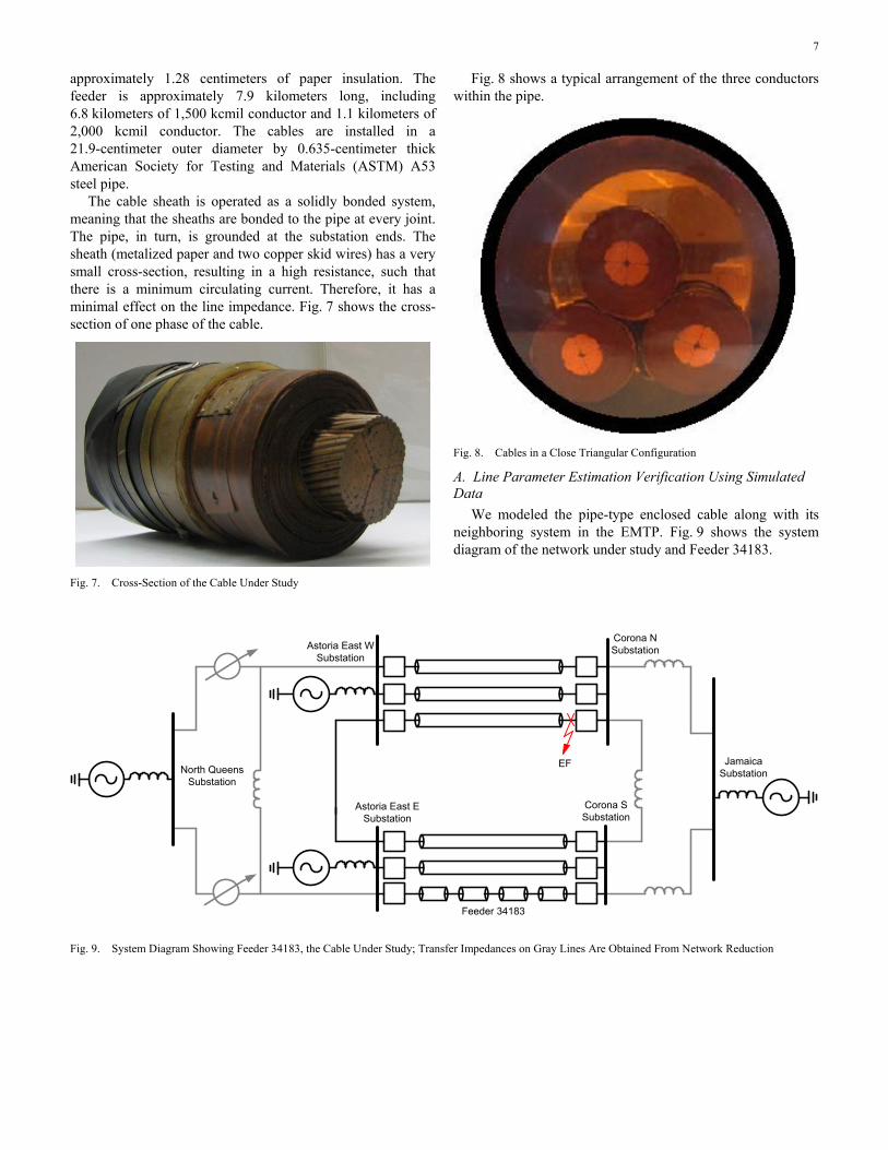
Fig. 8 shows a typical arrangement of the three conductors within the pipe.

Fig. 8. Cables in a Close Triangular Configuration

A. Line Parameter Estimation Verification Using Simulated Data

We modeled the pipe-type enclosed cable along with its neighboring system in the EMTP. Fig. 9 shows the system diagram of the network under study and Feeder 34183.

EF

Astoria East E Substation

Astoria East W Substation

Corona N Substation

Corona S Substation

Jamaica SubstationNorth Queens

Substation

Feeder 34183

Fig. 9. System Diagram Showing Feeder 34183, the Cable Under Study; Transfer Impedances on Gray Lines Are Obtained From Network Reduction

8

We simulated normal load conditions and recorded three-phase voltage and current measurements at the Astoria East and Corona terminals to measure positive-sequence line parameters. Simulated data are generated at 8,000 samples per second and are processed using a low-pass filter and resampled to 32 samples per cycle. A cosine filter is then used to extract the fundamental quantity of the signal and filter out dc and harmonics. The cosine-filtered signal is then used to construct the phasors that are used to estimate the line parameters. Fig. 10 shows the signal processing flow.

Terminal 1 Data

Terminal 2 Data

TimeAlignment

Low-PassFilterand

Resampler

CosineFilter

Phasors CalculateLine Parameters

Fig. 10. Signal Processing to Compute Line Parameters

1) Positive-Sequence Line Parameters We simulated 200 A of loading on the cable and recorded

the phase voltages and currents at both terminals. Equations (7) and (8) were used to calculate the positive-sequence line impedance and capacitance based on the data corresponding to this condition. Fig. 11 shows the comparison of the positive-sequence line impedance against the positive-sequence impedance value provided by the LCC program. We did not simulate CT, coupling capacitor voltage transformer (CCVT), and relay measurement errors for this analysis.

1.4

1.2

1

0.8

0.6

0.4

0.2

00 0.2 0.4 0.6 0.8 1

Rea

ctan

ce (Ω

)

Resistance (Ω)

Positive-Sequence Line Impedance From LCC Program

Fig. 11. Comparison of the Positive-Sequence Line Impedance Against the Line Parameters Reported by the LCC Program

Table VII shows the estimated positive-sequence line parameters using the pi model approach as compared with the parameters provided by the LCC program associated with the EMTP.

TABLE VII COMPARISON OF ESTIMATED POSITIVE-SEQUENCE LINE PARAMETERS

Positive-Sequence Parameters Measured LCC EMTP

Resistance (Ω) 0.4323 0.4324

Reactance (Ω) 0.9663 0.9664

Capacitance (μF) 2.87 2.8744

2) Zero-Sequence Line Parameters We simulated an external phase-to-ground fault at location

EF on the parallel line shown in Fig. 9 and recorded the phase voltages and currents at the Astoria East and Corona terminals. Equations (9) and (10) were used to calculate the zero-sequence line impedance and capacitance based on the data obtained during the fault condition. Due to the short fault duration, only a few cycles of data were available to estimate the zero-sequence line parameters. This method is prone to errors, specifically for short-duration faults where the phasor estimate is not stable. Fig. 12 shows the comparison of the zero-sequence line impedance against the line parameters provided by the LCC program. We calculated zero-sequence parameters for each sample during the fault. Fig. 12 shows the zero-sequence impedance estimate for each sample. Table VIII shows the estimated zero-sequence line parameters (mean value) using the pi model approach as compared with the parameters provided by the LCC program associated with the EMTP.

0 0.5 1 1.5 20

0.2

0.4

0.6

0.8

1

1.2

1.4

Resistance (Ω)

Rea

ctan

ce (Ω

)

Zero-Sequence Line Impedance From LCC Program

Fig. 12. Comparison of the Zero-Sequence Line Impedance Against the Line Parameters Reported by the LCC Program

TABLE VIII COMPARISON OF ESTIMATED ZERO-SEQUENCE LINE PARAMETER

Zero-Sequence Parameters Measured LCC EMTP

Resistance (Ω) 1.53 1.5303

Reactance (Ω) 1.07 1.061

Capacitance (μF) 3.53 3.45

9

Simulation results show that the methods discussed provide an accurate estimation of the line parameters. The following section discusses validating these methods using field measurements from Feeder 34183.

B. Line Parameter Estimation Verification Using Field Data We need time-synchronized measurements to compute the

line parameters using (7), (8), (9), and (10). We estimated the underground cable positive-sequence parameters by using time-synchronized oscillography data triggered from the relays installed at both ends of the cable during normal loading conditions. The oscillography data are a snapshot of the instantaneous samples of sending and receiving end voltage/current quantities. As mentioned in Section III, Subsection C, synchrophasor measurements are another source for time-synchronized measurements. We programmed the local and remote relays with logic to simultaneously trigger oscillography without interfering with the protection functions of the relays. Event reports are configured for 0.5 seconds of length at 8,000 samples per second. The user has to press a pushbutton on the front panel on one of the relays, which asserts a trigger bit to trigger the oscillography data from the local relay. This trigger bit is also communicated to the remote relay to trigger oscillography at the remote terminal. Additional triggers are configured to

trigger events automatically for external faults to provide the data required to compute the zero-sequence impedance of the cable. Fig. 13 shows the protection and recording system. The relays shown provide current differential protection.

A total of nine sets of event reports were triggered during normal operating conditions. The nine event pairs were grouped into three, based on the date of trigger. Table IX lists the positive-sequence load current along with the date associated with each event.

TABLE IX EVENTS RECORDED FOR CALCULATION OF LINE PARAMETERS

Event Date Load Current (A)

1 9/18/2014 264

2 9/18/2014 240

3 9/18/2014 227

4 9/18/2014 226

5 11/12/2014 212

6 11/12/2014 213

7 11/12/2014 217

8 11/12/2014 217

9 7/21/2014 206

GPS Receiver

Multiplexer 1

Multiplexer 2

Multiplexer 1

Multiplexer 2

RelayRelay

GPS Receiver

Astoria East Substation

Underground Pipe-Type Cable

Corona Substation

T1 Line

T1 Line

1200/5 A

138 kV/67 V

2000/5 A

138 kV/67 V

2000/5 A

6

5 8

7

Fig. 13. Protection and Event Recording System

10

1) Positive-Sequence Line Parameters From Field Data We read each event pair and time-aligned the data to

account for different trigger times. The time-aligned event data were then processed using the implementation described in Section VI, Subsection A, to extract the time-synchronized voltage and current phasors from both terminals. Equations (7) and (8) were executed using the phasor data. Fig. 14 shows the positive-sequence resistance and reactance measured using the nine event pairs as compared with the line resistance and reactance used by Con Edison.

0 0.1 0.2 0.3 0.4 0.50

0.2

0.4

0.6

0.8

1

1.2

1.4

Rea

ctan

ce (Ω

)

Resistance (Ω)

Line Impedance Used by Con Edison

Fig. 14. Comparison of the Positive-Sequence Line Impedance Against the Line Impedance Used by Con Edison

Fig. 15 shows the measured shunt capacitance for each sample using the nine event pairs. Measured capacitance is validated using the charging current recorded during cable energization.

0 200 400 6002.9

2.95

3

3.05

3.1

3.15

3.2

Data Samples

µF

Fig. 15. Measured Positive-Sequence Line Capacitance

Table X shows the summary of the cable parameters estimated using the nine event pairs. For each event pair we show the mean value of the line parameters.

TABLE X SUMMARY OF ESTIMATED LINE PARAMETERS

Event Event Date R (Ω) X (Ω) C (μF)

1 9/18/2014 0.35 1.17 3.07

2 9/18/2014 0.36 1.18 3.07

3 9/18/2014 0.36 1.17 3.07

4 9/18/2014 0.36 1.17 3.07

5 11/12/2014 0.34 1.16 3.07

6 11/12/2014 0.33 1.16 3.07

7 11/12/2014 0.34 1.16 3.07

8 11/12/2014 0.33 1.16 3.07

9 7/21/2014 0.32 1.15 3.07

Table XI shows the Feeder 34183 line parameters based on Neher’s formulae. These parameters are used by Con Edison for EMTP studies, line protection, and fault location.

TABLE XI LINE PARAMETER VALUES USED BY CON EDISON FOR FEEDER 34183

R (Ω) X (Ω) C (µF)

Positive Sequence 0.286 1.238 3.064

Zero Sequence 5.998 2.323 3.064

The recording system is configured to trigger event reports for external events to provide data for validating the zero-sequence impedance estimation method.

2) Line Capacitance Estimate Using Energization Data Event data were triggered at Astoria East during cable

energization with the Corona terminal open. Fig. 16 shows phase voltages and currents recorded during this energization event.

200

100

0

–100

–200

050

100150

–50–100–150

Cur

rent

(A)

Volta

ge (k

V)

Time (seconds)

1:IA_A 134.35 A

18.640916 18.680916 18.720916

18.640916 18.680916 18.720916

1:VA_kV 115.541 kV

Fig. 16. Phase Voltages and Currents Captured at the Astoria Terminal During Cable Energization

11

The following data are from the captured event shown in Fig. 16:

• Vpeak is 115.541 kV. • Ipeak is 134.35 A. • Peak current leads peak voltage by 4.166 milliseconds

or about 90 degrees (4.166 • 360/16.666 milliseconds = 89.99 degrees).

The event data from Fig. 16 were used to calculate line capacitance based on (11), as shown in (12).

( )

3

134.35• sin 89.99C F 3.084 F

2 • • 60 •115.541•10= = µ

π (12)

The measured capacitance from the line energization test is within 0.5 percent of the capacitance estimation using the pi model approach shown in Table X.

VII. CONCLUSION Accurate line parameters are required for line protection,

fault location, EMTP studies, and GIC flow estimation. LCC provides estimates of line parameters based on conductor spacing and properties. Dedicated injection devices and methods are available to measure the line parameters.

We discussed challenges in estimating line parameters for underground cables. Line protection devices have capabilities to provide time-synchronized measurements, providing users an economical and convenient means to estimate line parameters. We used field data recorded from a 138 kV cable installation to estimate the positive-sequence line impedance. Voltage and current data recorded from a line energization event were used to calculate the line charging capacitance. To estimate zero-sequence line parameters, we discussed a method that uses event data recorded from both terminals of the cable for an external event. We used data from EMTP simulations to validate this method. A protection and recording system is configured to trigger events from external events to compute zero-sequence impedance using field data.

VIII. APPENDIX

A. Calculation of Pipe-Type Cable Impedances Positive-sequence resistance is:

( )1 dc c s pR R 1 Y Y Y / foot= + + + µΩ (13)

where: Rdc = conductor dc resistance μΩ per foot. Yc = increment in losses due to conductor ac effects (dimensionless). Ys = increment in losses due to shield ac effects (dimensionless). Yp = increment in losses due to pipe ac effects (dimensionless).

Positive-sequence reactance is:

1 10c

2.57SX 60.9log / footD

= µΩ

(14)

where: S = axial spacing between phases. Dc = diameter of cable conductor in inches.

2

s6sp s

DS 1.26D 1– inches

D – D

=

(15)

where: Ds = diameter of skid wires in inches. Dp = pipe inside diameter in inches.

Therefore, the positive-sequence impedance is:

( )1 dc c s p 10c

2.57SZ R 1 Y Y Y j60.9 logD

= + + + +

(16)

B. Zero-Sequence Impedance Neher’s formula for zero-sequence impedance of pipe-type

cable Z0 is given in (17).

( )0 p c pZ 3 Rc / 3 R j X X / foot ′ ′= + + + µΩ (17)

where: Rc = conductor ac resistance (1 + Yc)Rdc μΩ per foot. R′p = pipe effective resistance in μΩ per foot. Xc = conductor ac reactance in μΩ per foot. X′p = pipe effective reactance in μΩ per foot.

IX. REFERENCES [1] A. Dierks, H. Troskie, and M. Krüger, “Accurate Calculation and

Physical Measurement of Transmission Line Parameters to Improve Impedance Relay Performance,” proceedings of the IEEE Power Engineering Society Inaugural Conference and Exposition in Africa, Durban, South Africa, July 2005.

[2] M. Grobler and R. Naidoo, “Determining Transmission Line Parameters From GPS Time-Stamped Data,” proceedings of the 32nd Annual Conference on IEEE Industrial Electronics, Paris, France, November 2006.

[3] R. Abboud, W. F. Soares, and F. Goldman, “Challenges and Solutions in the Protection of a Long Line in the Furnas System,” proceedings of the 32nd Annual Western Protective Relay Conference, Spokane, WA, October 2005.

[4] J. Roberts, A. Guzmán, and E. O. Schweitzer, III, “Z = V/I Does Not Make a Distance Relay,” proceedings of the 20th Annual Western Protective Relay Conference, Spokane, WA, October 1993.

[5] H. E. Prado-Félix, V. H. Serna-Reyna, M. V. Mynam, M. Donolo, and A. Guzmán, “Improve Transmission Fault Location and Distance Protection Using Accurate Line Parameters,” proceedings of the 40th Annual Western Protective Relay Conference, Spokane, WA, October 2013.

[6] North American Electric Reliability Corporation, 2012 Special Reliability Assessment Interim Report: Effects of Geomagnetic Disturbances on the Bulk Power System, February 2012. Available: https://www.frcc.com/Public%20Awareness/Lists/Announcements/ Attachments/105/GMD%20Interim%20Report.pdf.

12

[7] R. Horton, D. H. Boteler, T. J. Overbye, R. Pirjola, and R. C. Dugan, “A Test Case for the Calculation of Geomagnetically Induced Currents,” IEEE Transactions on Power Delivery, Vol. 27, Issue 4, October 2012, pp. 2368–2373.

[8] A. Amberg, A. Rangel, and G. Smelich, “Validating Transmission Line Impedances Using Known Event Data,” proceedings of the 65th Annual Conference for Protective Relay Engineers, College Station, TX, April 2012.

[9] D. Shi, D. J. Tylavsky, N. Logic, and K. M. Koellner, “Identification of Short Transmission-Line Parameters From Synchrophasor Measurements,” proceedings of the 40th North American Power Symposium, Calgary, Canada, September 2008.

[10] D. A. Tziouvaras, “Protection of High-Voltage AC Cables,” proceedings of the 59th Annual Conference for Protective Relay Engineers, College Station, TX, April 2006.

[11] J. H. Neher, “The Phase Sequence Impedance of Pipe-Type Cables,” IEEE Transactions on Power Apparatus and Systems, Vol. 83, Issue 8, August 1964, pp. 795−804.

[12] J. H. Neher and M. H. McGrath, “The Calculation of the Temperature Rise and Load Capability of Cable Systems,” Transactions of the American Institute of Electrical Engineers Power Apparatus and Systems, Part III, Vol. 76, Issue 3, April 1957, pp. 752–764.

X. BIOGRAPHIES Hibourahima Camara received his B.S. degree in electrical engineering from the City College of New York in 2001 and an M.S. in electrical engineering from the State University of New York (SUNY) at New Paltz in 2008. In December 2012, he received his professional engineer (PE) certification in New York. He joined IBM, Microelectronics Division, in Fishkill, New York in 2001. In his 10-year tenure with the company, he worked as a High-Speed Analog/Mixed-Signal Designer, designing serial-deserializer (SERDES) chips operating at data rates up to 40 Gbps. He joined the Con Edison Transmission Planning Department in January 2011 and has transferred to Control Systems Engineering where he has been working as a relay protection engineer since June 2013. He holds four U.S. patents in high-speed analog/mixed-signal design.

Jasvinder Blah received his B.S. degree in electrical engineering from the City College of New York in 2004. In 2010, he received his Project Management Professional (PMP) certification from the Project Management Institute (PMI). He joined Con Edison in 2004 as a GOLD associate. In 2005, he successfully completed the program and joined the Protective Systems and Testing (PST) department within Substation Operations, where he has been working as a Technical Supervisor designing test plans and commissioning various transmission and area stations.

Diego Pichardo received his B.S. degree in Electrical Engineering from the University of Rhode Island in 2005. He joined Con Edison in 2006 as an electrical technician and in 2009 held a title of increasing responsibility in the Protective Systems and Testing (PST) department as a senior electrical technician. In 2013, he joined the Technical Application Group as a Technical Supervisor within PST.

Arnold Wong received his B.S.E.E. from the Polytechnic Institute of Brooklyn in 1975. He is a graduate of the U.S. Army Command and General Staff College and U.S. Army Basic and Advanced Engineer Officers courses. He is a Project Manager for Con Edison with 30 years of experience in designing, constructing, and operating the Con Edison transmission system. He is the company subject matter expert for underground transmission including high-pressure pipe-type cables, self-contained fluid filled and solid dielectric cables installed in pipe and manhole duct systems, submarine, tunnel, and aerial installations. He is also responsible for the electric design of overhead transmission projects. He is a senior member of IEEE.

Amitabha Mukhopadhyay, P.E., received his B.S.E.E. from the University of Calcutta, India, and M.S.E.E. from the Polytechnic Institute of New York. He is a Senior Engineer for Con Edison with 35 years of experience in designing, constructing, and operating the Con Edison high-voltage substations and the transmission systems. He is the company subject matter expert (SME) for Overhead Transmission System, EMF, and Grounding. He received an Electric Power Research Institute (EPRI) Innovators and Technology Transfer Award. He is a New York State licensed professional engineer.

Mangapathirao V. Mynam received his M.S.E.E. from the University of Idaho in 2003 and his B.E. in electrical and electronics engineering from Andhra University College of Engineering, India, in 2000. He joined Schweitzer Engineering Laboratories, Inc. (SEL) in 2003 as an associate protection engineer in the engineering services division. He is presently working as a senior research engineer in SEL research and development. He was selected to participate in the U.S. National Academy of Engineering (NAE) 15th Annual U.S. Frontiers of Engineering Symposium. He is a senior member of IEEE.

Hang Li received his M.S.E.E from the University of Idaho in 2014 and his B.S. in electrical and electronics engineering from Washington State University in 2012. He joined Schweitzer Engineering Laboratories, Inc. as a research engineering intern in protection systems research of the research and development division in 2014. He is currently an associate power engineer in the power systems department. He is a member of IEEE.

Rogerio Scharlach received his B.S.E.E. from the University Mackenzie, Brazil, in 1991. Upon graduating, he served nearly 13 years at Siemens in Brazil and the United States, where he worked as a commissioning and field service engineer in the areas of power generation, transmission, and distribution. He joined Schweitzer Engineering Laboratories, Inc. in 2005 as a field application engineer.

© 2015 by Consolidated Edison Company of New York and Schweitzer Engineering Laboratories, Inc.

All rights reserved. 20150309 • TP6692-01