63668030 feedback control of dynamic systems 2008
TRANSCRIPT


I. Introduction

9/23/2009 I. Introduction 3
Introduction
• Aim of the course– Give a general overview of classical and modern
control theory– Give a general overview of modern control tools
• Prerequisites– Mathematics : complex numbers, linear algebra

9/23/2009 I. Introduction 4
Introduction
• Tools– Matlab / Simulink
• Book– « Feedback Control of Dynamics Systems », Franklin,
Powell, Amami-Naeini, Addison-Wessley Pub Co– Many many books, websites and free references...

9/23/2009 I. Introduction 5
Introduction
270 BC : the clepsydra and other hydraulically regulated devices for time measurement (Ktesibios)

9/23/2009 I. Introduction 6
Introduction
1136-1206 : Ibn al-Razzaz al-Jazari
“The Book of Knowledge of Ingenious Mechanical Devices” � crank mechanism, connecting rod, programmable automaton, humanoid robot, reciprocating piston engine, suction pipe, suction pump, double-acting pump, valve, combination lock, cam, camshaft, segmental gear, the first mechanical clocks driven by water and weights, and especially the crankshaft, which is considered the most important mechanical invention in history after the wheel
9/23/2009 I. Introduction 7
Introduction
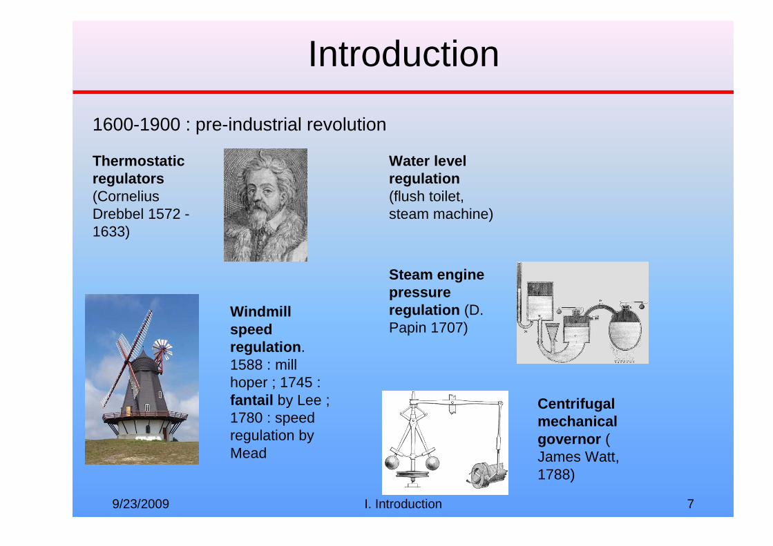
1600-1900 : pre-industrial revolution
Thermostatic regulators(Cornelius Drebbel 1572 -1633)
Windmill speed regulation. 1588 : mill hoper ; 1745 : fantail by Lee ; 1780 : speed regulation by Mead
Water level regulation (flush toilet, steam machine)
Steam engine pressure regulation (D. Papin 1707)
Centrifugal mechanical governor (James Watt, 1788)

9/23/2009 I. Introduction 8
Introduction
1800-1935 : mathematics, basis for control theory
Differential equations � first analysis and proofs of stability condition for feedback systems (Lagrange, Hamilton, Poncelet, Airy-1840, Hermite-1854, Maxwell-1868, Routh-1877, Vyshnegradsky-1877, Hurwitz-1895, Lyapunov-1892)
Frequency domain approach (Minorsky-1922, Black-1927, Nyquist-1932, Hazen-1934)
1940-1960 : classical period
Frequency domain theory : (Hall-1940, Nichols-194, Bode-1938)
Stochastic approach (Kolmogorov-1941, Wiener and Bigelow-1942)
Information theory (Shannon-1948) and cybernetics (Wiener-1949)
9/23/2009 I. Introduction 9
Introduction
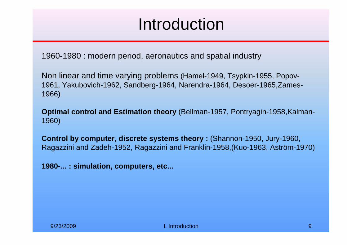
1960-1980 : modern period, aeronautics and spatial industry
Non linear and time varying problems (Hamel-1949, Tsypkin-1955, Popov-1961, Yakubovich-1962, Sandberg-1964, Narendra-1964, Desoer-1965,Zames-1966)
Optimal control and Estimation theory (Bellman-1957, Pontryagin-1958,Kalman-1960)
Control by computer, discrete systems theory : (Shannon-1950, Jury-1960, Ragazzini and Zadeh-1952, Ragazzini and Franklin-1958,(Kuo-1963, Aström-1970)
1980-... : simulation, computers, etc...

9/23/2009 I. Introduction 10
Introduction
What is automatic control ?
� Basic idea is to enhance open loop control with feedback control� This seemingly idea is tremendously powerfull� Feedback is a key idea in control
Open loop
Controler Process Input Output Input reference
Perturbation
Closed loop
Controler Process Input Output Input reference
Measurement
Perturbation

9/23/2009 I. Introduction 11
Introduction
Example : the feedback amplifier
Harold Black, 1927
A
R2
R1
V1 V2 + - Amplifier A has a high gain (say 40dB)
1R
2R
1R2R
1A1
1
1
1R
2R
1V
2V −≈
++⋅−=
Resulting gain is determined by passive components !� amplification is linear� reduced delay� noise reduction

9/23/2009 I. Introduction 12
Introduction
Use of block diagrams
� Capture the essence of behaviour� standard drawing� abstraction� information hiding� points similarities between systems
Same tools for :� generation and transmission of energy� transmission of informaiton� transportation (cars, aerospace, etc...)� industrial processes, manufacturing� mechatronics, instrumentation� Biology, medicine, finance, economy...

9/23/2009 I. Introduction 13
Introduction
Basic properties of feedback (1)
A V1
k
V2 -
+
( )( )
k
1
kA1
1
1
k
1
1V
2V
1VAkA12V
2Vk1VA2V
≈
⋅+
⋅=
⋅=⋅+⋅⋅−⋅=
� Resulting gain is determined by feedback !

9/23/2009 I. Introduction 14
Introduction
Basic properties of feedback (2) : static properties
kp r
- kc
e u
d
y
kp kc e u
d
y r : referencee : errord : disturbancey : outputkc : control gainKp : process gain
Open loop control : dkekky pcp ⋅+⋅⋅=
Closed loop control :p c p
p c p c
k k ky r d
1 k k 1 k k
⋅= ⋅ + ⋅
+ ⋅ + ⋅
� If kc is big enough y tend to r and d is rejected

9/23/2009 I. Introduction 15
Introduction
Basic properties of feedback (2) : dynamics properties
Closed loop control can :� enhance system dynamics� stabilize an unstable system� make unstable a stable system ! �

9/23/2009 I. Introduction 16
Introduction
The On-Off or bang-bang controller : u = {umax , umin}
e
u
e
u
e
u
The proportional controller : u=kc.(r – y)

9/23/2009 I. Introduction 17
Introduction
The proportional derivative controller
( ) ( ) ( )dt
tdektektu dp ⋅+⋅=
Gives an idea of future : phase advance
The proportional derivative controller
( ) ( ) ( )dt
tdektektu dp ⋅+⋅=
The proportional integral controller
( ) ( ) ( )∫ τ⋅τ⋅+⋅= t
0ip dektektu
e(t) tends to zero !

9/23/2009 II. A first controller design 18
II. A first controller design
9/23/2009 II. A first controller design 19
A first control design
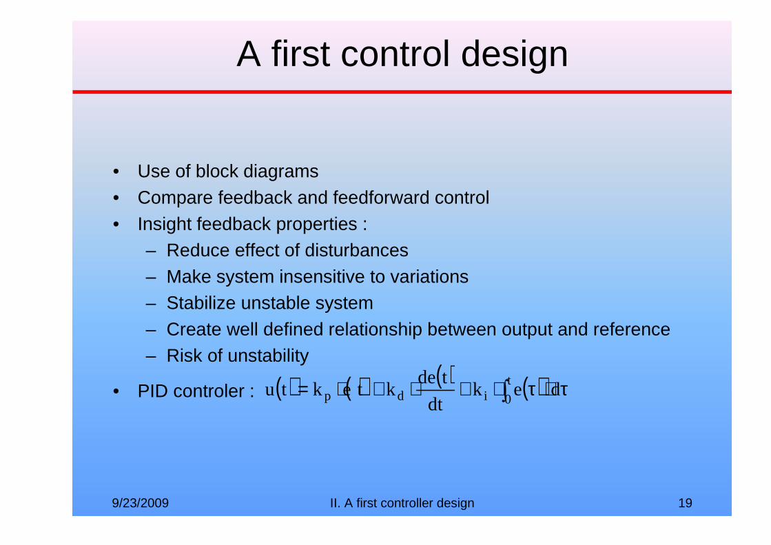
• Use of block diagrams• Compare feedback and feedforward control• Insight feedback properties :
– Reduce effect of disturbances– Make system insensitive to variations– Stabilize unstable system– Create well defined relationship between output and reference– Risk of unstability
• PID controler : ( ) ( ) ( ) ( )∫ τ⋅τ⋅+⋅+⋅= t
0idp dekdt
tdektektu

9/23/2009 II. A first controller design 20
Cruise control
mg
F
θθθθ
A cruise control problem :• Process input : gas pedal u• Process output : velocity v• Reference : desired velocity vr
• Disturbance : slope θ
Construct a block diagram• Understand how the system works• Identify the major components and the relevant signals• Key questions are :
– Where is the essential dynamics ?
– What are the appropriate abstractions ?
• Describe the dynamics of the blocks

9/23/2009 II. A first controller design 21
Cruise control
We made the assumptions :• Essential dynamics relates velocity to force• The force respond instantly to a change in the throttle• Relations are linear
Body vr
- Engine
F
ext. force
Controller v
Throttle
We can now draw the process equations

9/23/2009 II. A first controller design 22
Cruise control
Process linear equations :
( ) θ⋅⋅−=⋅+⋅ gmFvkdt
tdvm
Reasonable parameters according to experience :
( ) θ⋅−=⋅+ 10uv02.0dt
tdv
Where : • v in m.s-1
• u : normalized throttle 0 < u < 1
• θ slope in rad

9/23/2009 II. A first controller design 23
Cruise control
Process linear equations :
PI controller :
( ) θ⋅−=⋅+ 10uv02.0dt
tdv
( ) ( )( ) ( )( )∫ τ⋅τ−⋅+−⋅= t
0 rir dvvktvvktu
Combining equations leads to :
( ) ( ) ( ) ( ) ( )dt
tdtek
dt
tdek
dt
tedi
θ⋅=⋅+⋅++ 1002.02
2
Integral action
Steady state and θ = 0 � e = 0 !

9/23/2009 II. A first controller design 24
Cruise control
Now we can tune k and ki in order to achieve a given dynamics
( ) ( ) ( ) ( ) ( )dt
td10tek
dt
tdek02.0
dt
tedi
2 θ⋅=⋅+⋅++
( ) ( ) ( ) 0txdt
tdx2
dt
txd 200
2
=⋅ω+⋅ω⋅σ⋅+
How to choose ω0 and σ ?

9/23/2009 II. A first controller design 25
Cruise control
Compare open loop and closed loop
Open loop
Closed loop
9/23/2009 II. A first controller design 26
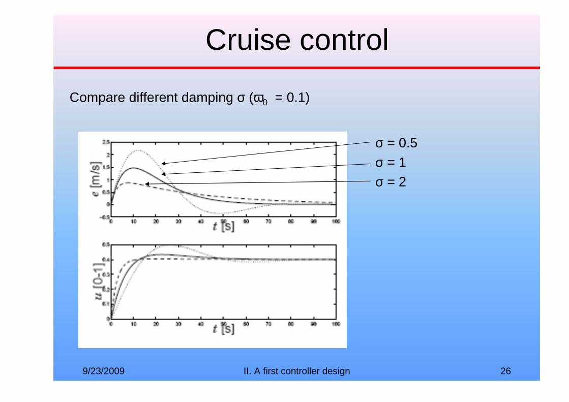
Cruise control
Compare different damping σ (ω0 = 0.1)
σ = 0.5σ = 1σ = 2

9/23/2009 II. A first controller design 27
Cruise control
Compare different natural frequencies ω0 (σ= 1)
ω0 = 0.05ω0 = 0.1ω0 = 0.2

9/23/2009 II. A first controller design 28
Cruise control
Control tools and methods help to :• Derive equations from the system• Manipulate the equations• Understand the equations (standard model)
– Qualitative understanding concepts
– Insight
– Standard form– Computations
• Find controller parameters• Validate the results by simulation
END 1

9/23/2009 II. A first controller design 29
Standard models
Standard models are foundations of the “control language”Important to :� Learn to deal with standard models� Transform problems to standard model
The standard model deals with Linear Time Invariant process (LTI), modelized with Ordinary Differential Equations (ODE) :
( ) ( ) ( ) ( ) ( )tub...dt
tudbtya...
dt
tyda
dt
tydn1n
1n
1n1n
1n
1n
n
⋅+⋅=⋅+⋅+ −
−
−
−
9/23/2009 II. A first controller design 30
Standard models
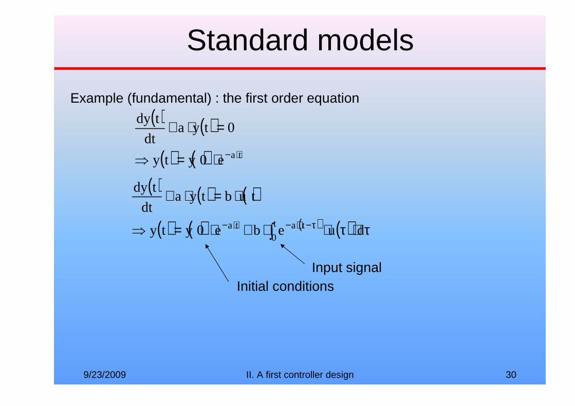
Example (fundamental) : the first order equation
( ) ( )
( ) ( ) tae0yty
0tyadt
tdy
⋅−⋅=⇒
=⋅+
( ) ( ) ( )
( ) ( ) ( ) ( ) τ⋅τ⋅⋅+⋅=⇒
⋅=⋅+
∫ τ−⋅−⋅− duebe0yty
tubtyadt
tdy
t
0tata
Input signalInitial conditions

9/23/2009 II. A first controller design 31
Standard models
A higher degree model is not so different :
( ) ( ) ( ) 0tya...dt
tyda
dt
tydn1n
1n
1n
n
=⋅+⋅+ −
−
Characteristic polynomial is :
( ) n1n
1n a...sassA +⋅+= −
If polynomial has n distinct roots αk then the time solution is :
( ) ∑=
⋅α⋅=n
1k
tk
keCty

9/23/2009 II. A first controller design 32
Standard models
Real αk roots gives first order responses :
Complex αk=σ±i.ω roots gives second order responses :

9/23/2009 II. A first controller design 33
Standard models
General case (input u) :
( ) ( ) ( ) ( ) ( )
( ) ( ) ( )∫∑ τ⋅τ−+⋅=⇒
⋅+⋅=⋅+⋅+
=
⋅α
−
−
−
−
t
0
n
1k
tk
n1n
1n
1n1n
1n
1n
n
dtgetCty
tub...dt
tudbtya...
dt
tyda
dt
tyd
k
Where : • Ck(t) are polynomials of t
• ( ) ( )∑=
⋅α⋅=n
1k
tk' ketCtg
A system is stable if all poles have negative real parts

9/23/2009 II. A first controller design 34
Standard models
Transfer function
� without knowing anything about Laplace transform it can be useful to store ak and bk coefficients in a convenient way, the transfer function :
( ) ( )( ) n
1n1
n1n
1n
b...sb
a...sas
sA
sBsF
+⋅+⋅+== −
−

9/23/2009 III. Laplace transforms 35
III. The Laplace transform

9/23/2009 III. Laplace transforms 36
• We assume the system to be LINEAR and TIME INVARIANT
The output (y) of the the system is related to the input (u) by the convolution :
Systemu y
Laplace transform (1) : convolution
dττ)h(t)u(τy(t) ⋅−⋅= ∫+∞
∞−
• Example : u(t) is an impulsion (0 everywhere except in t = 0)
h(t)y(t) =h(t) is called the impulse response, h(t) describes completelythe system
• Causality : h(t) = 0 if t < 0
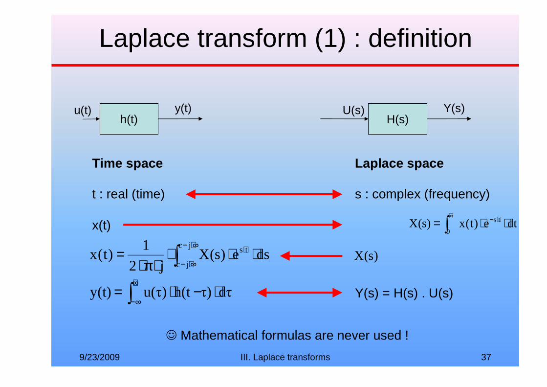
9/23/2009 III. Laplace transforms 37
Time space
h(t)u(t) y(t)
Laplace space
x(t)
H(s)U(s) Y(s)
Laplace transform (1) : definition
∫+∞ ⋅− ⋅⋅=0
ts dte)t(x)s(X
t : real (time) s : complex (frequency)
∫ ∞⋅−
∞⋅−
⋅ ⋅⋅⋅⋅π⋅
=jc
jc
ts dse)s(Xj2
1)t(x )s(X
dττ)h(t)u(τy(t) ⋅−⋅= ∫+∞
∞−Y(s) = H(s) . U(s)
☺ Mathematical formulas are never used !

9/23/2009 III. Laplace transforms 38
Step fonction :t<0 : x(t) = 0t>0 : x(t) = 1
X(s) = 1/s
Impulse fonctiont=0 : x(t)= infinitex(t)=0
X(s) = 1
Derivation :
)t(xdt
dy(t) = )0(x)s(X.s)s(Y +−=
Sinusoïdal fonction :
)tsin(y(t) ⋅ω= 22s
1)s(Y
ω+=
Laplace transform (2) : properties

9/23/2009 III. Laplace transforms 39
Delay :
)tt(xy(t) d−= stde)s(X)s(Y ⋅−⋅=
Initial value theorem :( )( )sYslim)0y(
s⋅=
∞→+
Final value theorem (if limit exists) :
( )( )sYslim)y(0s
⋅=∞+→
Laplace transform (3) : properties

9/23/2009 III. Laplace transforms 40
From t to s
Laplace transform (4) : tables

9/23/2009 III. Laplace transforms 41
From s to t
Laplace transform (4) : tables
9/23/2009 III. Laplace transforms 42
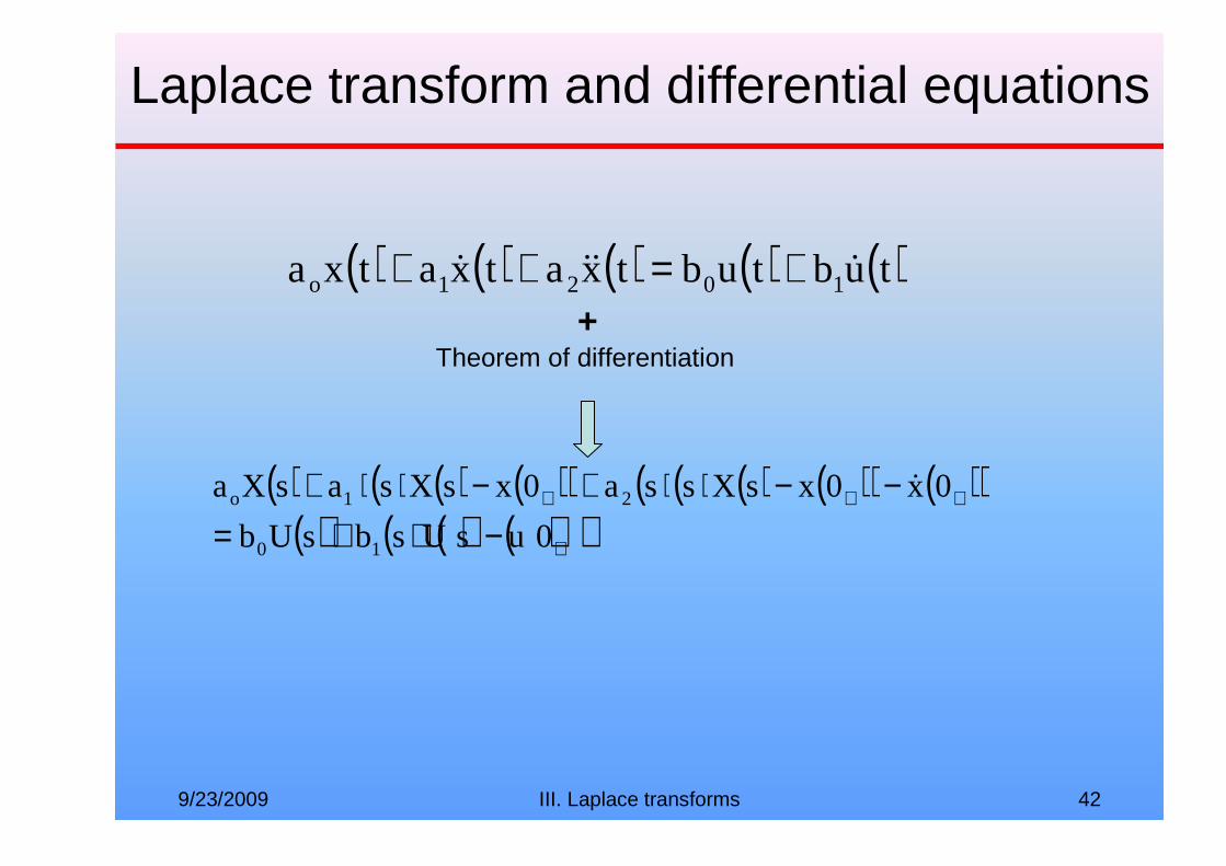
( ) ( ) ( ) ( ) ( )tubtubtxatxatxa 1021o ���� +=+++
Theorem of differentiation
( ) ( ) ( )( ) ( ) ( )( ) ( )( )( ) ( ) ( )( )+
+++
−⋅+=−−⋅⋅+−⋅⋅+
0usUsbsUb
0x0xsXssa0xsXsasXa
10
21o �
Laplace transform and differential equations

9/23/2009 III. Laplace transforms 43
( ) ( ) ( )( ) ( ) ( )( ) ( )( )( ) ( ) ( )( )+
+++
−⋅+=−−⋅⋅+−⋅⋅+
0usUsbsUb
0x0xsXssa0xsXsasXa
10
21o �
( ) ( ) ( ) ( ) ( )( ) ( ) ( )+
++
⋅−⋅⋅+=⋅−⋅⋅+−⋅⋅+⋅+
0ubsUsbb
0xa0xsaasXsasaa
110
2212
21o �
( ) ( ) ( ) ( ) ( ) ( )2
21o
12212
21o
10
sasaa
0ub0xa0xsaasU
sasaa
sbbsX
⋅+⋅+⋅−⋅+⋅⋅++
⋅+⋅+⋅+= +++ �
Initial conditions
Transfer function
Laplace transform and differential equations

9/23/2009 III. Laplace transforms 44
( ) ( ) ( ) ( )sIsUsHsX +⋅=
( ) ( ) ( ) ( ) ( ) ( )2
21o
12212
21o
10
sasaa
0ub0xa0xsaasU
sasaa
sbbsX
⋅+⋅+⋅−⋅+⋅⋅++
⋅+⋅+⋅+= +++ �
( ) ( ) ( ) ( )tituthtx +∗=
☺ Initial conditions are generally assumed to be null !
Laplace transform and differential equations

9/23/2009 III. Laplace transforms 45
Systemu(t) y(t)
What is the output y(t) from a given input u(t) ?
u(t)
Table of transform
U(s)Y(s) = H(s) . U(s)
Y(s)
y(t)
Table of transform
Finding output response with Laplace transform

9/23/2009 III. Laplace transforms 46
Systemu(t) y(t)
What is the final output y(inf) from a given input u(t) ?
u(t)
Table of transform
U(s)Y(s) = H(s) . U(s)
Y(s)
Theorem of final value
( )( )sYslim)y(0s
⋅=∞+→
Finding final value with Laplace transform

9/23/2009 III. Laplace transforms 47
Poles and zeros
H(s)YU
Transfer function is a ratio of polynomials :
...sasasaa
...sbsbb
)s(D
)s(N)s(H
)s(U
)s(Y3
32
210
2210
+++++++
===
Poles and zeros :( ) ( )
( ) ( ) ( ) ⋅⋅⋅−⋅−⋅−⋅⋅⋅−⋅−
⋅==321
21
0
0
pspsps
zszs
a
b)s(H
)s(U
)s(Yzero : z1, z2, …
poles : p1, p2, p3…
p2
p1 z1
Re
Im
p3
z2
• Poles and zeros are either into the left plane ore into the right plane
• Complex poles and zeros have a conjugate

9/23/2009 III. Laplace transforms 48
• Poles are the roots of Transfer functiondenominator– Real values or conjugate complex pairs
• Poles are also the eigenvalues of matrix A• Poles = modes

9/23/2009 III. Laplace transforms 49
Poles and zeros : decomposition
H(s)YU
Transfer function can be expansed into a sum of elementary terms :
...sasasaa
...sbsbb)s(H
)s(U
)s(Y3
32
210
2210
+++++++
==
...pspsps
)s(H)s(U
)s(Y
3
3
2
2
1
1 +−α
+−α+
−α==
p1 and p2 are conjugate :θ⋅−θ⋅ ⋅ω−=⋅ω−= j
0j
01 e2p,ep
...psscos2s
)s(H)s(U
)s(Y
3
32
002
2,1 +−α
+ω+⋅θ⋅ω⋅+
α==
First orders
Second orders
☺ Complex system response is the sum of first order and second ordersystems responses

9/23/2009 III. Laplace transforms 50
Dynamic response of first order systems
YU
1ps
1)s(H
+=
( ) ( )sUps
1sY
1+=
Example 1 : impulse responseu(t) is an impulsion (0 everywhere, except in 0 : ∞)
u(t)
Table of transform
U(s)=1
Table of transform
( ) ( ) ( )sUsHsY ⋅=( )
1ps
1sY
+=
tp1e)t(y ⋅−=

9/23/2009 III. Laplace transforms 51
Dynamic response of first order systems
YU
1ps
1)s(H
+=
( ) ( )sUps
1sY
1+=
Example 2 : step responseu(t) is a step
u(t)
Table of transform Table of transform
( ) ( ) ( )sUsHsY ⋅=( )
s
1
ps
1sY
1
⋅+
=
( )tp
1
1e1p
1)t(y ⋅−−=
( )s
1sU =

9/23/2009 III. Laplace transforms 52
Properties of first order systems
YU
1ps
1)s(H
+=
Step response
t1 = 1/p1 is the time constant of the system :
after t = t1, 63% of the final value is obtained
( ) ( )sUps
1sY
1+=

9/23/2009 III. Laplace transforms 53
200
2 s2s
1)s(H
ω+⋅ω⋅σ⋅+=
Dynamic response of second order systems
YU
Example 1 : impulse responseu(t) is an impulsion (0 everywhere, except in 0 : ∞)
u(t)
Table of transform
U(s)=1
Table of transform
( ) ( ) ( )sUsHsY ⋅=
( )t1sine1
1)t(y 2
0t
20
à ⋅σ−ω⋅⋅σ−ω
= ⋅ω⋅σ−
200
2 s2s
1)s(Y
ω+⋅ω⋅σ⋅+=

9/23/2009 III. Laplace transforms 54
200
2 s2s
1)s(H
ω+⋅ω⋅σ⋅+=
Dynamic response of second order systems
YU
Example 2 : step responseu(t) is an step
u(t)
Table of transform
U(s)=1/s
Table of transform
( ) ( ) ( )sUsHsY ⋅=
( )( )σ+⋅σ−ω⋅⋅σ−ω
−= ⋅ω⋅σ− cosart1sine1
11)t(y 2
0t
20
à
s
1
s2s
1)s(Y
200
2⋅
ω+⋅ω⋅σ⋅+=

9/23/2009 III. Laplace transforms 55
Properties of second order systems
Step response :
σ is the damping factorω0 is the natural frequency
200
2 s2s
1)s(H
ω+⋅ω⋅σ⋅+= YU
( )( )σ+⋅σ−ω⋅⋅σ−ω
−= ⋅ω⋅σ− cosart1sine1
11)t(y 2
0t
20
à
20 1 σ−ω is the pseudo-frequency
5% of the final value is obtained after :
0%5
3t
ω⋅σ≈
overshoot
Overshoot increases as σ decreases

9/23/2009 III. Laplace transforms 56
Properties of second order systems
Step response (continued) :
200
2 s2s
1)s(H
ω+⋅ω⋅σ⋅+= YU
poles : θ±⋅ω−= ep 02,1 cos(θ)=σ
θ
ω0
Re
Im

9/23/2009 III. Laplace transforms 57
Stability
Re
Im
Un
stab
le
Sta
ble
unstable pole, deverges likeexp(t)
stable pole, decays likeexp(-4.t)
Any pole with positive real part is unstable
Any input (even small) will lead to instability
See animation

9/23/2009 III. Laplace transforms 58
« fast poles » vs « slow poles »
Re
Im
slow
fast
slow pole, decays likeexp(-t)constant time : t1 = 1s
fast pole, decays likeexp(-4.t)constant time : t1 = 4s
Fast poles can be neglected
See animation

9/23/2009 III. Laplace transforms 59
Effect of zeros
See animation
Re
Im
Zeros modify the transient response
• Fast zero : neglected
• Slow zero : transientresponse affected
• Positive zero : non minimal phase system, step responsestart out in the wrongdirection

9/23/2009 III. Laplace transforms 60
Ex. analysis of a feedback system
Process model :
( ) θ⋅−=⋅+ 10uv02.0dt
tdv
Transfer functions :
( ) ( ) ( )( ) ( ) ( )
θ⋅−=⋅+⋅
=⋅+⋅s10sV02.0sVs
sUsV02.0sVs
( )( ) ( )
( )( )
+−=
θ
+==
⇒s02.0
10
s
sV
s02.0
1sF
sU
sV

9/23/2009 III. Laplace transforms 61
Ex. analysis of a feedback system
Transfer function of the controller (PID) :
( ) ( ) ( ) ( )( )( ) s
1kskk
tE
tU
dtekdt
tdektektu
id
t
0id
⋅+⋅+=⇒
τ⋅⋅+⋅+⋅= ∫

9/23/2009 III. Laplace transforms 62
Ex. analysis of a feedback system
We can now combine transfer functions :
vr
- F
θ
PID v
u
e -10
( ) ( ) ( ) ( ) ( ) ( ) ( )sEsPIDsF1
10sV
sPIDsF1
1sV r ⋅
⋅+−+⋅
⋅+=

9/23/2009 IV. Design of simple feedbacks 63
IV. Design of simple feedback

9/23/2009 IV. Design of simple feedbacks 64
P(s)u y
Introduction
Standard problems are often first orders or second orders• Standard problem � standard solution
C(s)
d
r
-
( )as
bsP
+= ( )
212
21
asas
bsbsP
+⋅++=

9/23/2009 IV. Design of simple feedbacks 65
Control of a first order system
Most physical problems can be modeled as first order systems
( )as
bsP
+=
Step 1 : transform your problem in a first order problem :
( )s
kksC i+=
Step 2 : choose a PI controller
Step 3 : combine equations and tune k and in ki in order to achieve the desired closed loop behavior (mass-spring damper analogy)
( ) ( ) ( )( ) ( )
20
2
0
i
i
ss
21
s'b1K
s
kk
asb
1
s
kk
asb
sCsP1
sCsPsCL
ω+⋅
ωσ⋅+
⋅+⋅=
+⋅+
+
+⋅+=
⋅+⋅=

9/23/2009 IV. Design of simple feedbacks 66
200
2 s2s
1)s(H
ω+⋅ω⋅σ⋅+=
Dynamic response of second order systems
YU
Example 1 : impulse responseu(t) is an impulsion (0 everywhere, except in 0 : ∞)
u(t)
Table of transform
U(s)=1
Table of transform
( ) ( ) ( )sUsHsY ⋅=
( )t1sine1
1)t(y 2
0t
20
à ⋅σ−ω⋅⋅σ−ω
= ⋅ω⋅σ−
200
2 s2s
1)s(Y
ω+⋅ω⋅σ⋅+=

9/23/2009 IV. Design of simple feedbacks 67
200
2 s2s
1)s(H
ω+⋅ω⋅σ⋅+=
Dynamic response of second order systems
YU
Example 2 : step responseu(t) is an step
u(t)
U(s)=1/s
Table of transform
( ) ( ) ( )sUsHsY ⋅=
( )( )σ+⋅σ−ω⋅⋅σ−ω
−= ⋅ω⋅σ− cosart1sine1
11)t(y 2
0t
20
à
s
1
s2s
1)s(Y
200
2⋅
ω+⋅ω⋅σ⋅+=
Table of transform

9/23/2009 IV. Design of simple feedbacks 68
Properties of second order systems
Step response :
σ is the damping factorω0 is the natural frequency
200
2 s2s
1)s(H
ω+⋅ω⋅σ⋅+= YU
( )( )σ+⋅σ−ω⋅⋅σ−ω
−= ⋅ω⋅σ− cosart1sine1
11)t(y 2
0t
20
à
20 1 σ−ω is the pseudo-frequency
5% of the final value is obtained after :
0%5
3t
ω⋅σ≈
overshoot
Overshoot increases as σ decreases

9/23/2009 IV. Design of simple feedbacks 69
Properties of second order systems
Step response (continued) :
200
2 s2s
1)s(H
ω+⋅ω⋅σ⋅+= YU
poles : θ±⋅ω−= ep 02,1 cos(θ)=σ
θ
ω0
Re
Im

9/23/2009 IV. Design of simple feedbacks 70
Control of a second order system
Step 1 , step 2 : idem (PI controller)
Step 3 : Transfer function is now third order �
( ) ( ) ( )( ) ( ) ( )
ω+⋅
ωσ⋅+⋅+
⋅+⋅=⋅+
⋅=
20
2
0
ss
21sa1
s'b1K
sCsP1
sCsPsCL
2 dof (k and ki) : the full dynamics (order 3) cannot be totally chosen �

9/23/2009 IV. Design of simple feedbacks 71
Simulation tools
Matlab or Scilab
� Transfer function is a Matlab object� Adapted to transfer function algebra (addition, multiplication…)� Simulation, time domain analysis

9/23/2009 VI. Design of simple feedbacks (Ctd) 72
Conclusion
Laplace Transform+
Simulation tools� Design of simple feedbacks

9/23/2009 V. Frequency response 73
V. Frequency response

9/23/2009 V. Frequency response 74
Introduction
Frequency response :• One way to view dynamics• Heritage of electrical engineering (Bode)• Fits well block diagrams• Deals with systems having large order
– electronic feedback amplifier have order 50-100 !• input output dynamics, black box models, external
description• Adapted to experimental determination of dynamics

9/23/2009 V. Frequency response 75
The idea of black box
The system is a black box : forget about the internal details and focus only on the input-output behavior
�Frequency response makes a “giant table” of possible inputs-outputs pairs
�Test entries are enough to fully describe LTI systems ☺- Step response- Impulse response- sinusoids
Systemu y

9/23/2009 V. Frequency response 76
What is a LTI system
A Linear Time Invariant System is :• Linear
� If (u1,y1) and (u2,y2) are input-output pairs then (a.u1+ b.u2 , a.y1+ b.y2) is an input-output pair : Theorem of superposition
• Time Invariant� (u1(t),y1(t)) is an input-output pair then (u1(t-T),y1(t-T)) is an input-
output pair
The “giant table” is drastically simplified :
( ) ( )( ) ( ) ( )sUsHsY
dττuτthy(t)
⋅=⇒
⋅⋅−= ∫+∞∞−

9/23/2009 V. Frequency response 77
What is the Fourier Transform
Fourier’s idea : an LTI system is completely determined by its response to sinusoidal signals
• Transmission of sinusoid is given by G(jω)• The transfer function G(s) is uniquely given by its values on
the imaginary axes• Frequency response can be experimentally determined
The complex number G(jω) tells how a sinusoid propagates through the system in steady states :
( )( ) ( )( )( )ω⋅+⋅ω⋅ω⋅=⇒
⋅ω=jGargtsinjGy(t)
tsinu(t)
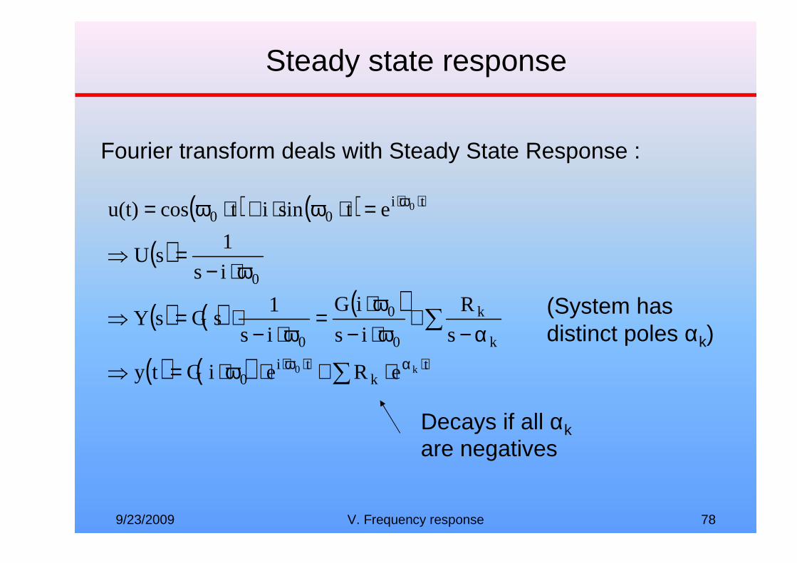
9/23/2009 V. Frequency response 78
Steady state response
( ) ( )( )
( ) ( ) ( )
( ) ( ) ∑∑
⋅α⋅ω⋅
⋅ω⋅
⋅+⋅ω⋅=⇒
α−+
ω⋅−ω⋅
=ω⋅−
⋅=⇒
ω⋅−=⇒
=⋅ω⋅+⋅ω=
tk
ti0
k
k
0
0
0
0
ti00
k0
0
eReiGty
s
R
is
iG
is
1sGsY
is
1sU
etsinitcosu(t)
Fourier transform deals with Steady State Response :
(System has distinct poles αk)
Decays if all αkare negatives
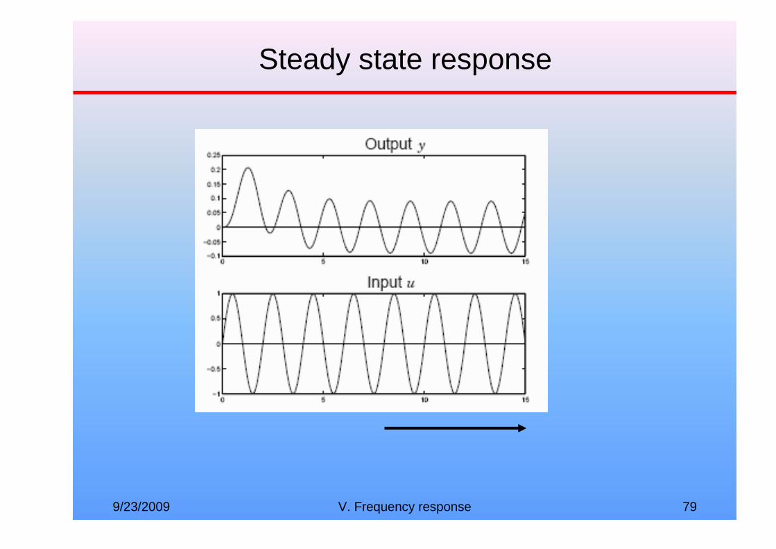
9/23/2009 V. Frequency response 79
Steady state response

9/23/2009 V. Frequency response 80
Nyquist stability theorem
Nyquist stability theorem tells if a system WILL BE stable (or not) with a simple feedback
L(s)=C(s).P(s)
-1
P(s).C(s).
-
(1) Standard system with negative unitary feedback
(2) Nyquist standard form
u(t) y(t)
(2) : if L(i.ω0) = -1 then oscillation will be maintained
y(t)

9/23/2009 V. Frequency response 81
Nyquist stability theorem
Step 1 : draw Nyquist curve
ω=0
Real
Imag
L(i.ω)ω=-∞
ω=+∞
Step 2 : where is (-1,0) ?

9/23/2009 V. Frequency response 82
Nyquist theorem
When the transfer loop function L does not have poles in the right half plane the closed loop system is stable if the complete Nyquist curve does not encircle the critical (-1,0) point.
When the transfer loop function L has N poles in the right half plane the closed loop system is stable if the complete Nyquist curve encircle the critical (-1,0) point N times.

9/23/2009 V. Frequency response 83
Nyquist stability theorem
Nyquist stability theorem compares L(i.ω) with (-1,0)
ω=0
Real
Imag
L(i.ω)
(-1,0)
(-1,0) (-1,0)
STABLE UNSTABLE

9/23/2009 V. Frequency response 84
Nyquist theorem
• Focus on the characteristic equation• Difficult to see how the characteristic equation L is influenced
by the controller C�Question is : how to change C ?
• Strong practical applications• Possibility to introduce stability margin : how close to
instability are we ?

9/23/2009 V. Frequency response 85
Stability margin
Stability margin definitions :
(-1,0) ϕM
1/gM
d
ϕM Phase margin
gM Gain margin
d Shortest distance to critical point
45°- 60°
2 - 6
0.5 - 0.8

9/23/2009 V. Frequency response 86
The Bode plot
Nyquist theorem is spectacular but not very efficient…� Impossible to distinguish C(s) and P(s)Bode plots two curves : one for gain, one for phase :
Logarithmic frequency axis
dB scale for gain
Linear scale for phase

9/23/2009 V. Frequency response 87
The Bode plot
Bode’s plot main properties :�Asymptotic curves (gain multiple of 20dB/dec) are ok�Simple interpretation of C(s) and P(s) in cascade :
GaindB(C(s).P(s) = GaindB(C(s)) + GaindB(P(s))
Phase(C(s).P(s) = Phase(C(s)) + Phase(P(s))

9/23/2009 V. Frequency response 88
The Bode stability criteria
Gain Margin > 0 : closed loop system will be stable
Phase Margin > 0 : closed loop system will be stable
One criteria is sufficient in most cases because gain and margin are closely related

9/23/2009 V. Frequency response 89
Typical property of Hbo(s) are :
( ) cbo for1jH ω<<ω>>ω⋅
( ) cbo for1jH ω>>ω<<ω⋅
( ) ( )( ) c
bo
bobf for1
jH1
jHjH ω<<ω≈
ω⋅+ω⋅=ω⋅
( ) ( )( ) ( ) cbo
bo
bobf forjH
jH1
jHjH ω>>ωω⋅≈
ω⋅+ω⋅=ω⋅
Close loop frequency response

9/23/2009 V. Frequency response 90
Log10ω
AdB
Open loop Bode plot
Close loop Bode plot
ωc
Close loop frequency response

9/23/2009 V. Frequency response 91
Log10ω
AdB
Open loop Bode plot
Close loop Bode plot (phase margin 90°)
ωc
Phase margin effect
Close loop Bode plot (phase margin 30°)
Close loop frequency response

9/23/2009 V. Frequency response 92
For small value of ω (low frequency) :
( ) ( )( )ω⋅+
ω⋅=ω⋅jH1
jHjH
bo
bobf
If Hbo(ω) >> 1 then Hbf(ω) ≅ 1
If Hbo(ω) → ∞ then Hbf(ω) → 1
If Hbo(ω) << 1 then Hbf(ω) ≅ Hbo(ω)
Static gain

9/23/2009 V. Frequency response 93
Controller specifications
C(s)u(s) y(s)e(s)
G(s)ε
-
Open loop transfer function : OLTF = C.GClose loop transfer function : CLTF = C.G / (1 + C.G)

9/23/2009 V. Frequency response 94
Controller specifications
• Static gain close to 1→ Low frequency : high gain
• Perturbation rejection→ High frequency : low gain
• Stability→ phase margin > 0
• Bandwith→ Cross over frequency ωc
• Overshoot ≈ 25%→ phase margin ≈ 45°→ Gentle slope in transition region
|C(jω).G(jω)|
ωc

9/23/2009 V. Frequency response 95
Controller design
• Proportionnal feedback– Effect : lifts gain with no
change in phase– Bode : shift gain by factor
of K
( ) KsC =

9/23/2009 V. Frequency response 96
Controller design
• Lead compensation– Effect : lifts phase by
increasing gain at highfrequency
– Very usefull controller : increase phase margin
– Bode : add phase betweenzero and pole
( )sA
sKsC
⋅⋅+⋅+=τ
τ1
1
9/23/2009 V. Frequency response 97
Modern loop shaping
• Use of rltool (Matlab Control Toolboxe)
9/23/2009 VI. Design of simple feedbacks (Ctd) 98
VI. Design of simple feedback (Ctd)

9/23/2009 VI. Design of simple feedbacks (Ctd) 99
P(s)u y
Introduction
More complete standard problem :
C(s)
d
-
n
e x
� Controller : feedback C(s) and feedforward F(s)� Load disturbance d : drives the system from its desired state x� Measurement disturbance n : corrupts information about x� Main requirement is that process variable x should follow reference r
F(s)r

9/23/2009 VI. Design of simple feedbacks (Ctd) 100
Introduction
Controller’s specifications :A. Reduce effects of load disturbanceB. Does not inject too much measurement noise into the systemC. Makes the closed loop insensitive to variations in the processD. Makes output follow reference signal
Classical approach : deal with A,B and C with controller C(s) and deal with D with feedforward F(s)

9/23/2009 VI. Design of simple feedbacks (Ctd) 101
Introduction
Controller’s specifications :A. Reduce effects of load disturbanceB. Does not inject too much measurement noise into the systemC. Makes the closed loop insensitive to variations in the processD. Makes output follow reference signal
Classical approach : deal with A,B and C with controller C(s) and deal with D with feedforward F(s) :
Design procedure• Design the feedback C(s) too achieve
– Small sensitivity to load disturbance d
– Low injection of measurement noise n
– High robustness to process variations
• Then design F(s) to achieve desired response to reference signal r

9/23/2009 VI. Design of simple feedbacks (Ctd) 102
Relations between signals
Three interesting signals (x, y, u)Three possible inputs (r, d, n)� Nine possible transfer functions !
rCP1
FCn
CP1
Cd
CP1
CPu
rCP1
FCPn
CP1
1d
CP1
Py
rCP1
FCPn
CP1
CPd
CP1
Px
⋅⋅+
⋅+⋅⋅+
+⋅⋅+
⋅=
⋅⋅+⋅⋅+⋅
⋅++⋅
⋅+=
⋅⋅+⋅⋅+⋅
⋅+⋅+⋅
⋅+=
� Six distinct transfer functions…

9/23/2009 VI. Design of simple feedbacks (Ctd) 103
Relations between signals
� Nine frequency responses…
-40
-20
0
From: dTo
: x
-40
-20
0
To: y
10-1
100
101
-40
-20
0
To: u
From: n
10-1
100
101
From: r
10-1
100
101
Bode Diagram
Frequency (rad/sec)
Mag
nitu
de (d
B)

9/23/2009 VI. Design of simple feedbacks (Ctd) 104
Relations between signals
� Nine step responses…
-2
0
2From: d
To:
x
-1
0
1
2
To:
y
0 10 20 30-2
0
2
To:
u
From: n
0 10 20 30
From: r
0 10 20 30
Step Response
Time (sec)
Am
plitu
de

9/23/2009 VI. Design of simple feedbacks (Ctd) 105
Relations between signals
A correct design means that each transfer has to be evaluated…� Need to be a little bit organized !� Need less criteria� Concept of sensibility functions

9/23/2009 VI. Design of simple feedbacks (Ctd) 106
Sensibility functions
rCP1
FCn
CP1
Cd
CP1
CPu
rCP1
FCPn
CP1
1d
CP1
Py
rCP1
FCPn
CP1
CPd
CP1
Px
⋅⋅+
⋅+⋅⋅+
+⋅⋅+
⋅=
⋅⋅+⋅⋅+⋅
⋅++⋅
⋅+=
⋅⋅+⋅⋅+⋅
⋅+⋅+⋅
⋅+=
CP1
CP
L1
LT
CP1
1
L1
1S
CPL
⋅+⋅=
+=
⋅+=
+=
⋅=
Sensibility function
Complementary sensibility function
Loop sensitivity function
L tells everything about stability : common denominator of each transfer functions

9/23/2009 VI. Design of simple feedbacks (Ctd) 107
Sensibility functions
L=PC tells everything about stability : common denominator of each transfer functions
-40
-20
0
Mag
nitu
de
(dB
)
10-1
100
10-360
-270
-180
-90
Pha
se (
deg)
Bode Diagram
Frequency (rad/sec)

9/23/2009 VI. Design of simple feedbacks (Ctd) 108
Sensibility functions
S=1/(1+L) tells about noise reduction
Pu y
C
d
-
n
e xr=0
Without feedback :
dPnyol ⋅+=
With feedback control :
olcl ySdCP1
Pn
CP1
1y ⋅=⋅
⋅++
⋅+=
� Disturbances with |S(iω)| < 1are reduced by feedback� Disturbances with |S(iω)| > 1are amplified by feedback

9/23/2009 VI. Design of simple feedbacks (Ctd) 109
Sensibility functions
It would be nice to have |S(iω)| < 1 for all frequencies !
Cauchy Integral Theorem :� for stable open loop system :
� For unstable or time delayed systems :
( ) 0iSlog0
=ω⋅∫∞( ) 0iSlog
0>ω⋅∫∞
Conclusion : water bed effect…
log|S(iω)|
ω

9/23/2009 VI. Design of simple feedbacks (Ctd) 110
Sensibility functions
Nyquist stability criteria :
(-1,0)
PC∆
L1d +=
T
1
P
P
L1PC,
<∆
⇔+<∆ω∀
� 1/T tells how much P is allowed to vary until system becomes unstable

9/23/2009 VI. Design of simple feedbacks (Ctd) 111
Sensibility functions
Nyquist stability criteria : � Minimum value of d tells how close
of instability is the system� dmin is a measure of robustness : the
bigger is M=1/d the more robust is the system
(-1,0)
PC∆
L1d +=
log|S(iω)|
ω
M

9/23/2009 VII. Feedforward design 112
VII. Feedforward design

9/23/2009 VII. Feedforward design 113
Introduction
Feedforward is a useful complement to feedback. Basic properties are:+ Reduce effects of disturbance that can be measured+ Improve response to reference signal+ No risk for instability- Design of feedforward is simple but requires good model and/or
measurements+ Beneficial when combined with feedback

9/23/2009 VII. Feedforward design 114
Attenuation of measured disturbance
P2
uP1
d
y
F
Disturbance is eliminated if F is chosen such as:F = P1
-1
� Need to measure d� P1 needs to be inversible
( )2 1Y
P 1 P FD
= ⋅ − ⋅

9/23/2009 VII. Feedforward design 115
Combined Feedback and Feedforward
P2
uP1
d
y
F
Disturbance d is attenuated both by F and C :
Cr
( )2 1P 1 P FY
D 1 P C
⋅ − ⋅=
+ ⋅

9/23/2009 VII. Feedforward design 116
System inverse
The ideal feedforward needs to compute the inverse of P1. That’s might be tricky… Examples:
( ) 1P s
1 s=
+( ) ( )1F s P s 1 s−= = +� Differentiation �
( )se
P s1 s
−=
+( ) ( ) ( )1 sF s P s 1 s e−= = + ⋅� Prediction �
( ) 1 sP s
1 s
−=+
( ) ( )1 1 sF s P s
1 s− += =
−� Unstable �

9/23/2009 VII. Feedforward design 117
Approximate system inverse
The ideal feedforward needs to compute the inverse of P1. That’s might be tricky… Examples:
( ) 1P s
1 s=
+( ) ( )1F s P s 1 s−= = +� Differentiation �
( )se
P s1 s
−=
+( ) ( ) ( )1 sF s P s 1 s e−= = + ⋅� Prediction �
( ) 1 sP s
1 s
−=+
( ) ( )1 1 sF s P s
1 s− += =
−� Unstable �

9/23/2009 VII. Feedforward design 118
Approximate system inverse
Since it is difficult to obtain an exact inverse we have to approximate. One possibility is to find the transfer function which minimizes :
( ) ( )( )0J u t v t dt∞= − ⋅∫
V P X U= ⋅ ⋅
Where:
And where U is a particular input (ex: a step signal). This gives for instance:
( ) 1P s
1 s=
+( )1 1 s
P s1 T s
− +≈+ ⋅�
( ) sP s e−= ( )1P s 1− ≈�
( ) 1 sP s
1 s
−=+
( ) ( )1F s P s 1−= =�

9/23/2009 VII. Feedforward design 119
Improved response to reference signal
The reference signal can be injected after the controller:
P2
ym yMy Cr
Mu
ym is the desired trajectory. Choose Mu = My / P
u
Design concerns:� Mu approximated� My adapted such that My/P feasible

9/23/2009 VII. Feedforward design 120
Combining feedback and feedforward
Feedback� Closed loop� Acts only when there are deviations� Market driven� Robust to model errors� Risk for instability
Feedforward� Open loop� Acts before deviation shows up� Planning� Not robust to model errors� No risk for instability
� Feedforward must be used as a complement to feedback. Requires good modeling.

9/23/2009 VIII. State feedback 121
VIII. State feedback

9/23/2009 VIII. State feedback 122
Introduction
- Simple design becomes difficult for high order systems- What is the State concept ?
- State are the variables that fully summarize the actual state of the system
- Future can be fully predicted from the current state- State is the ideal basis for control

9/23/2009 VIII. State feedback 123
State feedback
Let us suppose the system is described by the following equation (x is a vector, A, B and C are matrixes) :
dxA x B u
dty C x
= ⋅ + ⋅ = ⋅The general linear controller is :
u K x L u= − ⋅ + ⋅The closed loop system then becomes :
( ) ( )dxA x B K x L u A B K x B L u
dty C x
= ⋅ + ⋅ − ⋅ + ⋅ = − ⋅ ⋅ + ⋅ ⋅ = ⋅The closed loop system has the characteristic equation:
( ) ( )( )P s det s I A B K= ⋅ − − ⋅

9/23/2009 VIII. State feedback 124
State feedback
Let us suppose the system is described by the following equation (x is a vector, A, B and C are matrixes) :
dxA x B u
dty C x
= ⋅ + ⋅ = ⋅The general linear controller is :
u K x L u= − ⋅ + ⋅The closed loop system then becomes :
( ) ( )dxA x B K x L u A B K x B L u
dty C x
= ⋅ + ⋅ − ⋅ + ⋅ = − ⋅ ⋅ + ⋅ ⋅ = ⋅The closed loop system has the characteristic equation:
( ) ( )( )P s det s I A B K= ⋅ − − ⋅
Main mathematical tool is linear algebra and matrixes !

9/23/2009 VIII. State feedback 125
Pole placement
Original (open loop) system behavior depends on its poles, solution of the characteristic equation:
( ) ( )OLP s det s I A= ⋅ −
Closed loop system behavior depends on its poles, solution of the characteristic equation:
( ) ( )( )CLP s det s I A B K= ⋅ − − ⋅
Appropriate choice of K allow to place the poles anywhere ! (Needs simple mathematical skills (not detailed here ☺)
Needs to tune N parameters (N : dimension of x and K)
Two problems : observability, controllability

9/23/2009 VIII. State feedback 126
Pole placement
Poles of the OL system
Poles of the CL system

9/23/2009 VIII. State feedback 127
First problem : observability
In the control feedback equation x is supposed to be known. If one can access (measure) x, there is no problem. Sometimes, x cannot be measured but can be observed.
dxA x B u
dty C x
= ⋅ + ⋅ = ⋅System described by:
Only u and y accessible, A and B known. Solution is to estimate internal state x with a “state observer” of gain Ko :
( )obsobs obs obs
obs obs
dxA x B u K y y
dty C x
= ⋅ + ⋅ + ⋅ − = ⋅Appropriate choice of Kobs minimizes yobs – y : xobs tends to x
Poles of the observer are the poles of: ( ) ( )( )obsP s det s I A K C= ⋅ − − ⋅
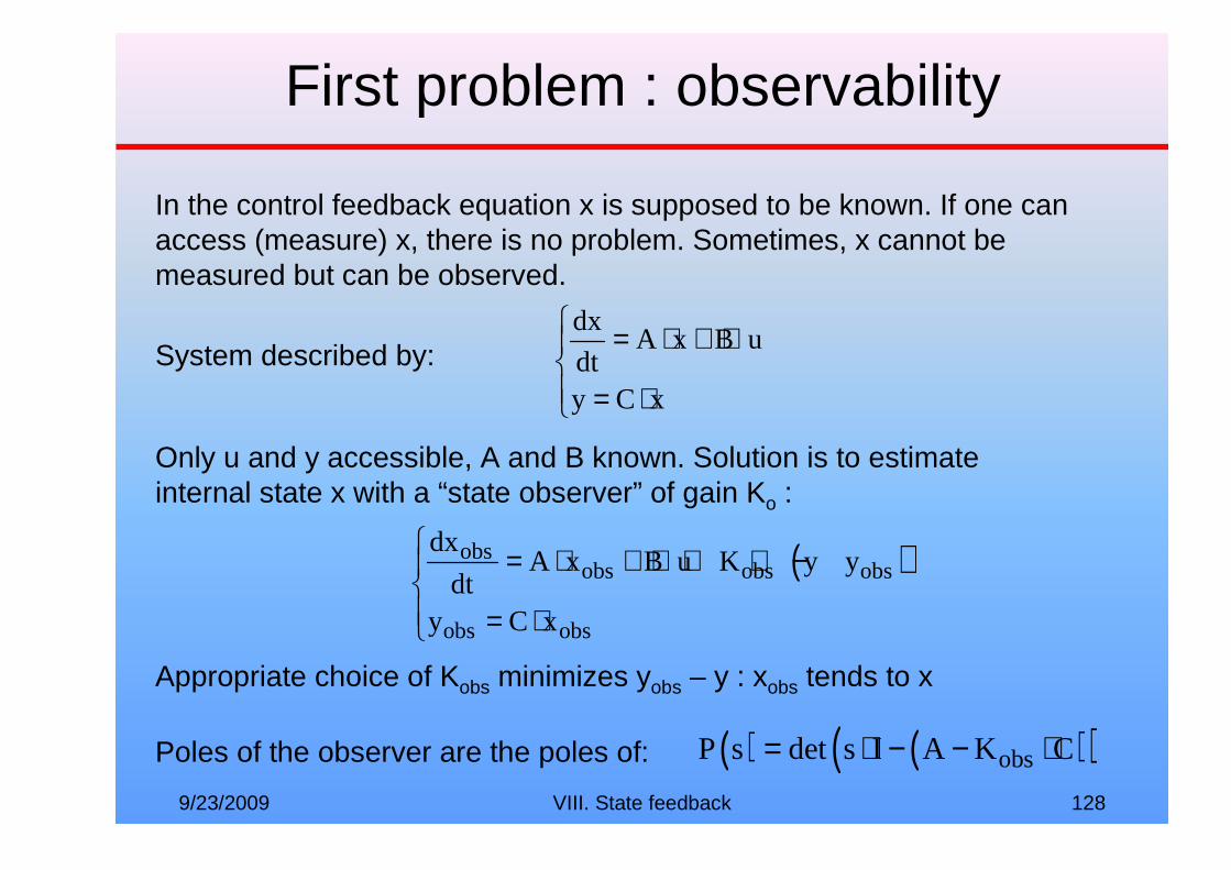
9/23/2009 VIII. State feedback 128
First problem : observability
In the control feedback equation x is supposed to be known. If one can access (measure) x, there is no problem. Sometimes, x cannot be measured but can be observed.
dxA x B u
dty C x
= ⋅ + ⋅ = ⋅System described by:
Only u and y accessible, A and B known. Solution is to estimate internal state x with a “state observer” of gain Ko :
( )obsobs obs obs
obs obs
dxA x B u K y y
dty C x
= ⋅ + ⋅ + ⋅ − = ⋅Appropriate choice of Kobs minimizes yobs – y : xobs tends to x
Poles of the observer are the poles of: ( ) ( )( )obsP s det s I A K C= ⋅ − − ⋅

9/23/2009 VIII. State feedback 129
First problem : observability
Poles of the observer are the poles those of:
( ) ( )( )obsP s det s I A K C= ⋅ − − ⋅Poles of the system
Poles of the observer

9/23/2009 VIII. State feedback 130
First problem : observability
Problem : is the system observable ?
In most cases : yes
Sometimes, the state is not observable :� The observer does not converge to the true state, whatever Kobs is.� Can be derived from a mathematical analyses of (A,C):
rank(A,AC,AAC,AAAC…) = N

9/23/2009 VIII. State feedback 131
Combining an observer and a state feedback
True (with x) state feedback can be replaced by an observed (xobs) state feedback:
obsu K x L u= − ⋅ + ⋅ Poles of the OL system
Poles of the observer
Poles of the CL system

9/23/2009 VIII. State feedback 132
Second problem : controllability
Sometimes a state is not controllable : means that whatever the command u is, some parts of the state are not controllable� Can be derived from a mathematical analyses of (A,B):
rank(A,AB,AAB,AAAB…) = N
Problem if :- A state is not controllable and unstable- A state is not controllable and slowNo problem if :- A state is not controllable and fast (decays rapidly)