Massachusetts Institute of TechnologyDepartment of Electrical Engineering and Computer Science

6.061 Introduction to Power SystemsClass Notes Chapter 9

Synchronous Machine and Winding Models ∗

J.L. Kirtley Jr.

1 Introduction

The objective here is to develop a simple but physically meaningful model of the synchronous machine, one of the major classes of electric machine. We can look at this model from several different directions. This will help develop an understanding of analysis of machines, particularly in cases where one or another analytical picture is more appropriate than others. Both operation and sizing will be of interest here.

Along the way we will approach machine windings from two points of view. On the one hand, we will approximate windings as sinusoidal distributions of current and flux linkage. Then we will take a concentrated coil point of view and generalize that into a more realistic and useful winding model.

2 Physical Picture: Current Sheet Description

Consider this simple picture. The ‘machine’ consists of a cylindrical rotor and a cylindrical stator which are coaxial and which have sinusoidal current distributions on their surfaces: the outer surface of the rotor and the inner surface of the stator.

The ‘rotor’ and ‘stator’ bodies are made of highly permeable material (we approximate this as being infinite for the time being, but this is something that needs to be looked at carefully later). We also assume that the rotor and stator have current distributions that are axially (z) directed and sinusoidal:

KzS = KS cos pθ

KzR = KR cos p (θ − φ)

Here, the angle φ is the physical angle of the rotor. The current distribution on the rotor goes along. Now: assume that the air-gap dimension g is much less than the radius: g << R. It is not

∗�2003 James L. Kirtley Jr.

1

c

Figure 1: Elementary Machine Model: Axial View

difficult to show that with this assumption the radial flux density Br is nearly uniform across the gap (i.e. not a function of radius) and obeys:

Then the radial magnetic flux density for this case is simply:

Now it is possible to compute the traction on rotor and stator surfaces by recognizing that the surface current distributions are the azimuthal magnetic fields: at the surface of the stator, HQ= -K:, and at the surface of the rotor, HQ= K;. So at the surface of the rotor, traction is:

TO= Tro= --P o R (Ks sinp0 + KR sinp (0 - 4)) KR cosp (0 - 4)Pg

The average of that is simply:

The same exercise done at the surface of the stator yields the same results (with opposite sign). To find torque, use:

We can pause here to make a few observations:

1. For a given value of surface currents Ks and Kr, torque goes as the fourth power of linear dimension. The volume of the machine goes as the third power, so this implies that torque capability goes as the 413 power of machine volume. Actually, this understates the situation

3

since the assumed surface current densities are the products of volume current densities and winding depth, which one would expect to increase with machine size. Thus machine torque (and power) densities tend to increase somewhat faster with size.

2. The current distributions want to align with each other. In actual practice what is done is to generate a stator current distribution which is not static as implied here but which rotates in space:

KS = KS cos (pθ − ωt)z

and this pulls the rotor along.

3. For a given pair of current distributions there is a maximum torque that can be sustained, but as long as the torque that is applied to the rotor is less than that value the rotor will adjust to the correct angle.

Continuous Approximation to Winding Patterns:

Now let’s try to produce those surface current distributions with physical windings. In fact we can’t do exactly that yet, but we can approximate a physical winding with a turns distribution that would look like:

nS = NS

2R cos pθ

nR = NR

2R cos p (θ − φ)

Note that this implies that NS and NR are the total number of turns on the rotor and stator. i.e.:

� π 2

p nSRdθ = NS π

−2

Then the surface current densities are as we assumed above, with:

NSIS NRIRKS = KR =

2R 2R

So far nothing is different, but with an assumed number of turns we can proceed to computing inductances. It is important to remember what these assumed winding distributions mean: they are the density of wires along the surface of the rotor and stator. A positive value implies a wire with sense in the +z direction, a negative value implies a wire with sense in the -z direction. That is, if terminal current for a winding is positive, current is in the +z direction if n is positive, in the -z direction if n is negative. In fact, such a winding would be made of elementary coils with one half (the negatively going half) separated from the other half (the positively going half) by a physical angle of π/p. So the flux linked by that elemental coil would be:

� θ

Φi(θ) = µ0Hr(θ�)�Rdθ�

θ−π/p

So, if only the stator winding is excited, radial magnetic field is:

NSISHr = −

2gp sin pθ

3

and thus the elementary coil flux is:

µ0NSIS�R Φi(θ) = cos pθ

p2g

Now, this is flux linked by an elementary coil. To get flux linked by a whole winding we must ‘add up’ the flux linkages of all of the elementary coils. In our continuous approximation to the real coil this is the same as integrating over the coil distribution:

� π 2p

λS = p Φi(θ)nS(θ)Rdθ π

− 2p

This evaluates fairly easily to: π �RNS

2

IsλS = µ0 4 gp2

which implies a self-inductance for the stator winding of:

π �RNS 2

LS = µ0 4 gp2

The same process can be used to find self-inductance of the rotor winding (with appropriate changes of spatial variables), and the answer is:

π �RNR 2

LR = µ0 24 gp

To find the mutual inductance between the two windings, excite one and compute flux linked by the other. All of the expressions here can be used, and the answer is:

π �RNSNRM(φ) = µ0

4 gp2 cos pφ

Now it is fairly easy to compute torque using conventional methods. Assuming both windings are excited, magnetic coenergy is:

1 1 W � LRIR

2 + M(φ)ISIR= m LSIS 2 +

2 2

and then torque is:∂W � π �RNSNR

ISIR sin pφ T = ∂φ

m = −µ0 4 gp

and then substituting for NSIS and NRIR:

NSIS = 2RKS

NRIR = 2RKR

we get the same answer for torque as with the field approach:

T = 2πR2� < τθ >= µ0πR

3�KSKR sin pφ

pg

4

� � � �

� �

� �

4

5

Classical, Lumped-Parameter Synchronous Machine:

Now we are in a position to examine the simplest model of a polyphase synchronous machine. Suppose we have a machine in which the rotor is the same as the one we were considering, but the stator has three separate windings, identical but with spatial orientation separated by an electrical angle of 120◦ = 2π/3. The three stator windings will have the same self- inductance (La).

With a little bit of examination it can be seen that the three stator windings will have mutual inductance, and that inductance will be characterized by the cosine of 120◦ . Since the physical angle between any pair of stator windings is the same,

1 Lab = Lac = Lbc = −

2 La

There will also be a mutual inductance between the rotor and each phase of the stator. Using M to denote the magnitude of that inductance:

π �RNaNfM = µ0

4 gp2

Maf = M cos (pφ) �

2π �

Mbf = M cos pφ − 3

� 2π �

Mcf = M cos pφ + 3

We show in Chapter 1 of these notes that torque for this system is:

2π 2π T = −pMiaif sin (pφ) − pMibif sin pφ − − pMicif sin pφ +

3 3

Balanced Operation:

Now, suppose the machine is operated in this fashion: the rotor turns at a constant velocity, the field current is held constant, and the three stator currents are sinusoids in time, with the same amplitude and with phases that differ by 120 degrees.

pφ = ωt + δi

if = If

ia = I cos (ωt)

2π ib = I cos ωt −

3 2π

ic = I cos ωt + 3

Straightforward (but tedious) manipulation yields an expression for torque:

3 T = −

2pMIIf sin δi

5

� �

� �

� �

Operated in this way, with balanced currents and with the mechanical speed consistent with the electrical frequency (pΩ = ω), the machine exhibits a constant torque. The phase angle δi is called the torque angle, but it is important to use some caution, as there is more than one torque angle.

Now, look at the machine from the electrical terminals. Flux linked by Phase A will be:

λa = Laia + Labib + Lacic + MIf cos pφ

Noting that the sum of phase currents is, under balanced conditions, zero and that the mutual phase-phase inductances are equal, this simplifies to:

λa = (La − Lab) ia + MIf cos pφ = Ldia + MIf cos pφ

where we use the notation Ld to denote synchronous inductance. Now, if the machine is turning at a speed consistent with the electrical frequency we say it is

operating synchronously, and it is possible to employ complex notation in the sinusoidal steady state. Then, note:

ia = I cos (ωt + θi) = Re Iejωt+θi

If , we can write an expression for the complex amplitude of flux as:

λa = Re Λaejωt

where we have used this complex notation:

I = Iejθi

If = Ifejθm

Now, if we look for terminal voltage of this system, it is:

dλa = Re jωΛ ejωt va =

dt a

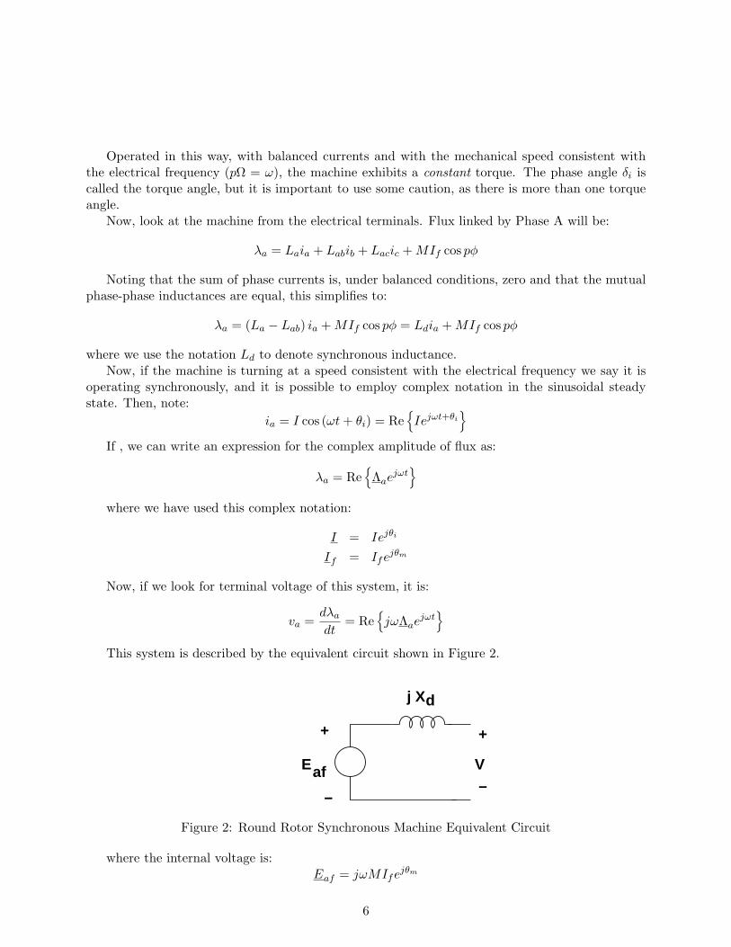
This system is described by the equivalent circuit shown in Figure 2.

j Xd

V

+

−

Eaf

+

−

Figure 2: Round Rotor Synchronous Machine Equivalent Circuit

where the internal voltage is: Eaf = jωMIfe

jθm

6

Now, if that is connected to a voltage source (i.e. if is fixed), terminal current is:

V − Eaf ejδ

I = jXd

where Xd = ωLd is the synchronous reactance. Then real and reactive power (in phase A) are:

1 V I∗P + jQ =

2 � �

∗

1 V −Eaf ejδ

= V 2 jXd

1 V 2 1 V Eafejδ

= 2 −

|jX

|d −

2 −jXd

This makes real and reactive power:

1 V EafPa = −

2 Xd sin δ

1 V 2 1 V Eaf XdQa =

2Xd −

2 cos δ

If we consider all three phases, real power is

3 V EafP = −

2 Xd sin δ

Now, at last we need to look at actual operation of these machines, which can serve either as motors or as generators.

Vector diagrams that describe operation as a motor and as a generator are shown in Figures 3 and 4, respectively.

Ia V V

δ

j X Id a

Iaδ

j X Id a

Eaf Eaf

Over−Excited Under−Excited

Figure 3: Motor Operation, Under- and Over- Excited

Operation as a generator is not much different from operation as a motor, but it is common to make notations with the terminal current given the opposite (“generator”) sign.

7

6

δ

Eaf

Ia

δ

Eaf

j X Id a j X Id a

V VIa

Over−Excited Under−Excited

Figure 4: Generator Operation, Under- and Over- Excited

Reconciliation of Models

We have determined that we can predict its power and/or torque characteristics from two points of view : first, by knowing currents in the rotor and stator we could derive an expression for torque vs. a power angle:

3 T = −

2pMIIf sin δi

From a circuit point of view, it is possible to derive an expression for power:

3 V Eaf P = −

2 Xd sin δ

and of course since power is torque times speed, this implies that:

3 V Eaf 3 pV Eaf T = −

2 ΩXd sin δ = −

2 ωXd sin δ

In this section of the notes we will, first of all, reconcile these notions, look a bit more at what they mean, and then generalize our simple theory to salient pole machines as an introduction to two-axis theory of electric machines.

6.1 Torque Angles:

Figure 5 shows a vector diagram that shows operation of a synchronous motor. It represents the MMF’s and fluxes from the rotor and stator in their respective positions in space during normal operation. Terminal flux is chosen to be ‘real’, or occupy the horizontal position. In motor operation the rotor lags by angle δ, so the rotor flux MIf is shown in that position. Stator current is also shown, and the torque angle between it and the rotor, δi is also shown. Now, note that the dotted line OA, drawn perpendicular to a line drawn between the stator flux LdI and terminal flux Λt, has length:

|OA| = LdI sin δi = Λt sin δ

8

7

Ld I

i

A

O t

M I f

Figure 5: Synchronous Machine Phasor Addition

Then, noting that terminal voltage V = ωΛt, Ea = ωMIf and Xd = ωLd , straightforward substitution yields:

3 pV Eaf 3 sin δ = pMIIf sin δi

2 ωXd 2

So the current- and voltage- based pictures do give the same result for torque.

Per-Unit Systems:

Before going on, we should take a short detour to look into per-unit systems, a notational device that, in addition to being convenient, will sometimes be conceptually helpful. The basic notion is quite simple: for most variables we will note a base quantity and then, by dividing the variable by the base we have a per-unit version of that variable. Generally we will want to tie the base quantity to some aspect of normal operation. So, for example, we might make the base voltage and current correspond with machine rating. If that is the case, then power base becomes:

PB = 3VBIB

and we can define, in similar fashion, an impedance base:

VBZB =

IB

Now, a little caution is required here. We have defined voltage base as line-neutral and current base as line current (both RMS). That is not necessary. In a three phase system we could very well have defined base voltage to have been line-line and base current to be current in a delta connected element:

IBVBΔ =

√3VB IBΔ = √

3

In that case the base power would be unchanged but base impedance would differ by a factor of three:

PB = VBΔIBΔ ZBΔ = 3ZB

9

8

However, if we were consistent with actual impedances (note that a delta connection of elements of impedance 3Z is equivalent to a wye connection of Z), the per-unit impedances of a given system are not dependent on the particular connection. In fact one of the major advantages of using a per-unit system is that per-unit values are uniquely determined, while ordinary variables can be line-line, line-neutral, RMS, peak, etc., for a large number of variations.

Perhaps unfortunate is the fact that base quantities are usually given as line-line voltage and base power. So that:

PB VB 1 VBΔ VB2ΔIB = √

3VBΔ

ZB = IB 3 IBΔ PB

= =

Now, we will usually write per-unit variables as lower-case versions of the ordinary variables:

V P v =

VB p =

PB etc.

Thus, written in per-unit notation, real and reactive power for a synchronous machine operating in steady state are:

2veaf v veaf p = sin δ q =−

xd xd −

xd sin δ

These are, of course, in motor reference coordinates, and represent real and reactive power into the terminals of the machine.

Normal Operation:

The synchronous machine is used, essentially interchangeably, as a motor and as a generator. Note that, as a motor, this type of machine produces torque only when it is running at synchronous speed. This is not, of course, a problem for a turbogenerator which is started by its prime mover (e.g. a steam turbine). Many synchronous motors are started as induction machines on their damper cages (sometimes called starting cages). And of course with power electronic drives the machine can often be considered to be “in synchronism” even down to zero speed.

As either a motor or as a generator, the synchronous machine can either produce or consume reactive power. In normal operation real power is dictated by the load (if a motor) or the prime mover (if a generator), and reactive power is determined by the real power and by field current.

Figure 6 shows one way of representing the capability of a synchronous machine. This picture represents operation as a generator, so the signs of p and q are reversed, but all of the other elements of operation are as we ordinarily would expect. If we plot p and q (calculated in the normal way) against each other, we see the construction at the right. If we start at a location q = −v2/xd, (and remember that normally v = 1 per-unit , then the locus of p and q is what would be obtained by swinging a vector of length veaf/xd over an angle δ. This is called a capability chart because it is an easy way of visualizing what the synchronous machine (in this case generator) can do. There are three easily noted limits to capability. The upper limit is a circle (the one traced out by that vector) which is referred to as field capability. The second limit is a circle that describes constant |p + jq|. This is, of course, related to the magnitude of armature current and so this limit is called armature capability. The final limit is related to machine stability, since the torque angle cannot go beyond 90 degrees. In actuality there are often other limits that can be represented on this type of a chart. For example, large synchronous generators typically have a problem with heating of the

10

9

Q

dX

1

P

Field Limit

Stator

Limit

Stability Limit

Figure 6: Synchronous Generator Capability Diagram

stator iron when they attempt to operate in highly underexcited conditions (q strongly negative), so that one will often see another limit that prevents the operation of the machine near its stability limit. In very large machines with more than one cooling state (e.g. different values of cooling hydrogen pressure) there may be multiple curves for some or all of the limits.

Another way of describing the limitations of a synchronous machine is embodied in the Vee

Curve. An example is shown in Figure 7 . This is a cross-plot of magnitude of armature current with field current. Note that the field and armature current limits are straightforward (and are the right-hand and upper boundaries, respectively, of the chart). The machine stability limit is what terminates each of the curves at the upper left-hand edge. Note that each curve has a minimum at unity power factor. In fact, there is yet another cross-plot possible, called a compounding curve, in which field current is plotted against real power for fixed power factor.

Salient Pole Machines: Two-Reaction Theory

So far, we have been describing what are referred to as “round rotor” machines, in which stator reactance is not dependent on rotor position. This is a pretty good approximation for large turbine generators and many smaller two-pole machines, but it is not a good approximation for many synchronous motors nor for slower speed generators. For many such applications it is more cost effective to wind the field conductors around steel bodies (called poles) which are then fastened onto the rotor body, with bolts or dovetail joints. These produce magnetic anisotropies into the machine which affect its operation. The theory which follows is an introduction to two-reaction theory and consequently for the rotating field transformations that form the basis for most modern dynamic analyses.

Figure 8 shows a very schematic picture of the salient pole machine, intended primarily to show how to frame this analysis. As with the round rotor machine the stator winding is located in slots in the surface of a highly permeable stator core annulus. The field winding is wound around steel pole pieces. We separate the stator current sheet into two components: one aligned with and one

11

Vee Curves

Per

-Un

it Ia

1.2

1

0.8

0.6

0.4

0.2

0

0 0.5 1 1.5 2 2.5 3

Per-Unit Field Current

Per-Unit Real Power: 0.00 0.32 0.64 0.96

Figure 7: Synchronous Machine Vee Curve

in quadrature to the field. Remember that these two current components are themselves (linear) combinations of the stator phase currents. The transformation between phase currents and the d-and q- axis components is straightforward and will appear in Chapter 4 of these notes.

The key here is to separate MMF and flux into two orthogonal components and to pretend that each can be treated as sinusoidal. The two components are aligned with the direct axis and with the quadrature axis of the machine. The direct axis is aligned with the field winding, while the quadrature axis leads the direct by 90 degrees. Then, if φ is the angle between the direct axis and the axis of phase a, we can write for flux linking phase a:

λa = λd cosφ − λq sinφ

Then, in steady state operation, if Va = dλa and φ = ωt + delta ,dt

Va = −ωλd sinφ − ωλq cosφ

which allows us to define:

Vd = −ωλq

Vq = ωλd

one might think of the ‘voltage’ vector as leading the ‘flux’ vector by 90 degrees.Now, if the machine is linear, those fluxes are given by:

λd = LdId + MIf

λq = LqIq

12

�

d−axis

Iq

q=axis Id

If

Figure 8: Cartoon of a Salient Pole Synchronous Machine

Vq

V d

V

Figure 9: Resolution of Terminal Voltage

Note that, in general, Ld = Lq. In wound-field synchronous machines, usually Ld > Lq. The reverse is true for most salient (buried magnet) permanent magnet machines.

Referring to Figure 9, one can resolve terminal voltage into these components:

Vd = V sin δ

Vq = V cos δ

or:

Vd = −ωλq = −ωLqIq = V sin δ

Vq = ωλd = ωLdId + ωMIf = V cos δ

which is easily inverted to produce:

Id = V cos δ −Eaf

Xd

13

V sin δ Iq = −

Xq

where Xd = ωLd Xq = ωLq Eaf = ωMIf

Now, we are working in ordinary variables (this discussion should help motivate the use of per­unit!), and each of these variables is peak amplitude. Then, if we take up a complex frame of reference:

V = Vd + jVq

I = Id + jIq

complex power is:

3 3 P + jQ = V I∗ =

2 {(VdId + VqIq) + j (VqId − VdIq)}

2

or: � � � �

P = − 3

2

V Eaf

Xd sin δ +

V 2

2

1

Xd − 1

Xq sin 2δ

� � � � � �

Q = 3

2

V 2

2

1

Xd +

1

Xq − V 2

2

1

Xd − 1

Xq cos 2δ − V Eaf

Xd cos δ

Id

d axis

j X I

j X I

j X Iq

q q

d d I

I

q

q axis

Eaf

Figure 10: Phasor Diagram: Salient Pole Machine

A phasor diagram for a salient pole machine is shown in Figure 10. This is a little different from the equivalent picture for a round-rotor machine, in that stator current has been separated into its d- and q- axis components, and the voltage drops associated with those components have

14

� �

�

been drawn separately. It is interesting and helpful to recognize that the internal voltage Eaf can be expressed as:

Eaf = E1 + (Xd −Xq) Id

where the voltage E1 is on the quadrature axis. In fact, E1 would be the internal voltage of a round rotor machine with reactance Xq and the same stator current and terminal voltage. Then the operating point is found fairly easily:

δ = − tan−1 XqI sinψ V + XqI cosψ

E1 = (V + XqI sinψ)2 + (XqI cosψ)2

Power-Angle Curves

-1.5

-1

-0.5

0

0.5

1

1.5

-4 -3 -2 -1 0 1 2 3 4Per

-Un

it Round Rotor

Salient Rotor

xd=2.2

xq = 1.6

Torque Angle

Figure 11: Torque-Angle Curves: Round Rotor and Salient Pole Machines

A comparison of torque-angle curves for a pair of machines, one with a round, one with a salient rotor is shown in Figure 11 . It is not too difficult to see why power systems analysts often neglect saliency in doing things like transient stability calculations.

10 Relating Rating to Size

It is possible, even with the simple model we have developed so far, to establish a quantitative relationship between machine size and rating, depending (of course) on elements such as useful flux

15

�

and surface current density. To start, note that the rating of a machine (motor or generator) is:

|P + jQ| = qV I

where q is the number of phases, V is the RMS voltage in each phase and I is the RMS current. To establish machine rating we must establish voltage and current, and we do these separately.

10.1 Voltage

Assume that our sinusoidal approximation for turns density is valid:

Na na(θ) = cos pθ

2R

And suppose that working flux density is:

Br(θ) = B0 sin p(θ − φ)

Now, to compute flux linked by the winding (and consequently to compute voltage), we first compute flux linked by an incremental coil:

� θ

λi(θ) = �Br(θ�)Rdθ�

θ−

Then flux linked by the whole coil is:

πp

π 2p π 2�RNa

λa = p λi(θ)na(θ)Rdθ = B0 cos pφ −

π 2p

4 p

This is instantaneous flux linked when the rotor is at angle φ. If the machine is operating at some electrical frequency ω with a phase angle so that pφ = ωt + δ, the RMS magnitude of terminal voltage is:

ω π B0Va =

p 42�RNa √

2

Finally, note that the useful peak current density that can be used is limited by the fraction of machine periphery used for slots:

B0 = Bs (1 − λs)

where Bs is the flux density in the teeth, limited by saturation of the magnetic material.

10.2 Current

The (RMS) magnitude of the current sheet produced by a current of (RMS) magnitude I is:

q NaI Kz =

2 2R

And then the current is, in terms of the current sheet magnitude:

2 I = 2RKz

qNa

16

Note that the surface current density is, in terms of area current density Js, slot space factor λs

and slot depth hs: Kz = λsJshs

This gives terminal current in terms of dimensions and useful current density:

4R I = λshsJs

qNa

10.3 Rating

Assembling these expressions, machine rating becomes:

ω Bs |P + jQ| = qV I = p

2πR2�√2 λs (1 − λs)hsJs

This expression is actually fairly easily interpreted. The product of slot factor times one minus slot factor optimizes rather quickly to 1/4 (when λs = 1). We could interpret this as:

∗ |P = jQ| = Asusτ

where the interaction area is: As = 2πR�

The surface velocity of interaction is:

ω R = ΩRus =

p

and the fragment of expression which “looks like” traction is:

∗ Bs

τ = hsJs √2 λs (1 − λs)

Note that this is not quite traction since the current and magnetic flux may not be ideally aligned, and this is why the expression incorporates reactive as well as real power.

This is not quite yet the whole story. The limit on Bs is easily understood to be caused by saturation of magnetic material. The other important element on shear stress density, hsJs is a little more involved.

We will do a more complete derivation of winding reactances shortly. Here, start by noting that the per-unit, or normalized synchronous reactance is:

I = µ0R λs √

2 hsJs

xd = XdV pg 1 − λs Bs

While this may be somewhat interesting by itself, it becomes useful if we solve it for hsJa:

p(1 − λs)BshsJa = xdg

µ0Rλs

√2

That is, if xd is fixed, hsJa (and so power) are directly related to air- gap g.Now, to get a limit on g, we must answer the question of how far the field winding can “throw” effective air- gap flux? To

17

�

understand this question, we must calculate the field current to produce rated voltage, no- load, and then the excess of field current required to accommodate load current.

Under rated operation, per- unit field voltage is:

eaf 2 = v 2 + (xdi)

2 + 2xdi sinψ

Or, if at rated conditions v and i are both unity (one per- unit), then

eaf = 1 + x2 d + 2xd sinψ

Thus, given a value for xd and ψ, per- unit internal voltage eaf is also fixed. Then field current required can be calculated by first estimating field winding current for “no-load operation”.

µ0NfIfnl Br =

2gp

and rated field current is: If = Ifnleaf

or, required rated field current is:

NfIf =2gp(1 − λp)Bs

eaf µ0

Next, If can be related to a field current density:

NRS NfIf = ARSJf

2

where NRS is the number of rotor slots and the rotor slot area ARS is

ARS = wRhR

where hR is rotor slot height and wR is rotor slot width:

2πR wR = λR

NRS

Then: NfIf = πRλRhRJf

Now we have a value for air- gap g:

2µ0kfRλRhRJf g =

p(1 − λs)Bseaf

This then gives us useful armature surface current density:

hsJs = √

2 xd λR

hRJf eaf λs

We will not have a lot more to say about this. Note that the ratio of xd/eaf can be quite small (if the per-unit reactance is small), will never be a very large number for any practical machine, and is generally less than one. As a practical matter it is unusual for the per-unit synchronous reatance of a machine to be larger than about 2 or 2.25 per-unit. What this tells us should be obvious: either the rotor or the stator of a machine can produce the dominant limitation on shear stress density (and so on rating). The best designs are “balanced”, with both limits being reached at the same time.

18

�

11 Winding Inductance Calculation

The purpose of this section is to show how the inductances of windings in round- rotor machines with narrow air gaps may be calculated. We deal only with the idealized air- gap magnetic fields, and do not consider slot, end winding, peripheral or skew reactances. We do, however, consider the space harmonics of winding magneto-motive force (MMF).

To start, consider the MMF of a full- pitch, concentrated winding. Assuming that the winding has a total of N turns over p pole- pairs, the MMF is:

∞ � 4 NI

F = sinnpφ nπ 2p

n = 1 nodd

This leads directly to magnetic flux density in the air- gap:

∞ � µ0 4 NI

sinnpφ Br = g nπ 2p

n = 1 nodd

Note that a real winding, which will most likely not be full- pitched and concentrated, will have a winding factor which is the product of pitch and breadth factors, to be discussed later.

Now, suppose that there is a polyphase winding, consisting of more than one phase (we will use three phases), driven with one of two types of current. The first of these is balanced, current:

Ia = I cos(ωt)

2π Ib = I cos(ωt − )

3 2π

Ic = I cos(ωt + ) (1) 3

Conversely, we might consider Zero Sequence currents:

Ia = Ib = Ic = I cosωt

Then it is possible to express magnetic flux density for the two distinct cases. For the balanced

case: ∞

Br = Brn sin(npφ � ωt) n=1

where

• The upper sign holds for n = 1, 7, ...

• The lower sign holds for n = 5, 11, ...

all other terms are zero •

19

�

and 3 µ0 4 NI

Brn = 2 g nπ 2p

The zero- sequence case is simpler: it is nonzero only for the triplen harmonics:

∞ � µ0 4 NI 3

g nπ 2p 2(sin(npφ − ωt) + sin(npφ + ωt)) Br =

n=3,9,...

Next, consider the flux from a winding on the rotor: that will have the same form as the flux produced by a single armature winding, but will be referred to the rotor position:

∞ � µ0 4 NI

Brf = sinnpφ� g nπ 2p

n = 1 nodd

ωt which is, substituting φ� = φ − p ,

∞ � µ0 4 NI

Brf = g nπ 2p

sinn(pφ − ωt)

n = 1 nodd

The next step here is to find the flux linked if we have some air- gap flux density of the form:

∞

Br = Brn sin(npφ ± ωt) n=1

Now, it is possible to calculate flux linked by a single- turn, full- pitched winding by:

� π p

φ = BrRldφ 0

and this is: ∞ � Brn

φ = 2Rl cos(ωt) np

n=1

This allows us to compute self- and mutual- inductances, since winding flux is:

λ = Nφ

The end of this is a set of expressions for various inductances. It should be noted that, in the real world, most windings are not full- pitched nor concentrated. Fortunately, these shortcomings can be accommodated by the use of winding factors.

The simplest and perhaps best definition of a winding factor is the ratio of flux linked by an actual winding to flux that would have been linked by a full- pitch, concentrated winding with the same number of turns. That is:

λactual kw =

λfull−pitch

20

�

�

It is relatively easy to show, using reciprocity arguments, that the winding factors are also the ratio of effective MMF produced by an actual winding to the MMF that would have been produced by the same winding were it to be full- pitched and concentrated. The argument goes as follows: mutual inductance between any pair of windings is reciprocal. That is, if the windings are designated one and two, the mutual inductance is flux induced in winding one by current in winding two, and it is also flux induced in winding two by current in winding one. Since each winding has a winding factor that influences its linking flux, and since the mutual inductance must be reciprocal, the same winding factor must influence the MMF produced by the winding.

The winding factors are often expressed for each space harmonic, although sometimes when a winding factor is referred to without reference to a harmonic number, what is meant is the space factor for the space fundamental.

Two winding factors are commonly specified for ordinary, regular windings. These are usually called pitch and breadth factors, reflecting the fact that often windings are not full pitched, which means that individual turns do not span a full π electrical radians and that the windings occupy a range or breadth of slots within a phase belt. The breadth factors are ratios of flux linked by a given winding to the flux that would be linked by that winding were it full- pitched and concentrated. These two winding factors are discussed in a little more detail below. What is interesting to note, although we do not prove it here, is that the winding factor of any given winding is the product of the pitch and breadth factors:

kw = kpkb

With winding factors as defined here and in the sections below, it is possible to define winding inductances. For example, the synchronous inductance of a winding will be the apparent induc­tance of one phase when the polyphase winding is driven by a balanced set of currents. This is, approximately:

∞ 3 4 µ0N2Rlk2

wn Ld = 2 π p2gn2

n=1,5,7,...

This expression is approximate because it ignores the asynchronous interactions between higher order harmonics and the rotor of the machine. These are beyond the scope of this note.

Zero- sequence inductance is the ratio of flux to current if a winding is excited by zero sequence currents:

∞ 4 µ0N2Rlk2

L0 = 3 wn

π p2gn2 n=3,9,...

And then mutual inductance, as between a field winding (f) and an armature winding (a), is:

∞ � 4 µ0NfNakfnkanRl

M(θ) = π p2gn2

cos(npθ)

n = 1 nodd

Now we turn out attention to computing the winding factors for simple, regular winding patterns. We do not prove but only state that the winding factor can, for regular winding patterns, be expressed as the product of a pitch factor and a breadth factor, each of which can be estimated separately.

21

�

�

� �

�

Pitch factor is found by considering the flux linked by a less- than- full pitched winding. Consider the situation in which radial magnetic flux density is:

Br = Bn sin(npφ − ωt)

A winding with pitch α will link flux:

π + α 2p 2p

λ = Nl Bn sin(npφ − ωt)Rdφπ−

α 2p 2p

Pitch α refers to the angular displacement between sides of the coil, expressed in electrical radians. For a full- pitch coil α = π.

The flux linked is: 2NlRBn nπ nα

λ = sin( ) sin( ) np 2 2

The pitch factor is seen to be: nα

kpn = sin 2

Now for breadth factor. This describes the fact that a winding may consist of a number of coils, each linking flux slightly out of phase with the others. A regular winding will have a number (say m) coil elements, separated by electrical angle γ.

A full- pitch coil with one side at angle ξ will, in the presence of sinusoidal magnetic flux density, link flux:

λ = Nlπp

ξ

p

− ξ

p

Bn sin(npφ − ωt)Rdφ

This is readily evaluated to be:

2NlRBn j(ωt−nξ)λ = Re enp

where complex number notation has been used for convenience in carrying out the rest of this derivation.

Now: if the winding is distributed into m sets of slots and the slots are evenly spaced, the angular position of each slot will be:

ξi = iγ − m − 1 γ

2

and the number of turns in each slot will be N , so that actual flux linked will be: mp

2NlRBn 1 m−1 �

j(ωt−nξi) �

λ = Re enp m

i=0

The breadth factor is then simply:

m−11 � m−1−jn(iγ−

2 γ)kb = e m

i=0

22

� � �

Note that this can be written as:

jnγ m−1 m e 2 � kb = e −jniγ

m i=0

Now, focus on that sum. We know that any coverging geometric sum has a simple sum:

∞ � 1i x =

x i=0

1 −

and that a truncated sum is: m−1 ∞ ∞

= −i=0 i=0 i=m

Then the useful sum can be written as:

m−1 � � ∞ jnmγ

� � ee −jniγ = 1 − ejnmγ e −jniγ =

1 −e−jnγ

i=0 i=0 1 −

Now, the breadth factor is found: sin nmγ

kbn = m sin

2 nγ 2

23

MIT OpenCourseWarehttp://ocw.mit.edu

6.061 / 6.690 Introduction to Electric Power SystemsSpring 2011

For information about citing these materials or our Terms of Use, visit: http://ocw.mit.edu/terms.