6 markov chains - jfet.org6 markov chains chap. 6 n-step transition probabilities many markov chain...
TRANSCRIPT

6
Markov Chains
Contents
6.1. Discrete-Time Markov Chains . . . . . . . . . . . . . . . p. 26.2. Classification of States . . . . . . . . . . . . . . . . . . . p. 96.3. Steady-State Behavior . . . . . . . . . . . . . . . . . . p. 136.4. Absorption Probabilities and Expected Time to Absorption . p. 256.5. More General Markov Chains . . . . . . . . . . . . . . . p. 33
1
2 Markov Chains Chap. 6
The Bernoulli and Poisson processes studied in the preceding chapter are memo-ryless, in the sense that the future does not depend on the past: the occurrencesof new “successes” or “arrivals” do not depend on the past history of the process.In this chapter, we consider processes where the future depends on and can bepredicted to some extent by what has happened in the past.
We emphasize models where the effect of the past on the future is summa-rized by a state, which changes over time according to given probabilities. Werestrict ourselves to models whose state can take a finite number of values andcan change in discrete instants of time. We want to analyze the probabilisticproperties of the sequence of state values.
The range of applications of the models of this chapter is truly vast. Itincludes just about any dynamical system whose evolution over time involvesuncertainty, provided the state of the system is suitably defined. Such systemsarise in a broad variety of fields, such as communications, automatic control,signal processing, manufacturing, economics, resource allocation, etc.
6.1 DISCRETE-TIME MARKOV CHAINS
We will first consider discrete-time Markov chains, in which the state changesat certain discrete time instants, indexed by an integer variable n. At each timestep n, the Markov chain has a state, denoted by Xn, which belongs to a finiteset S of possible states, called the state space. Without loss of generality, andunless there is a statement to the contrary, we will assume that S = {1, . . . , m},for some positive integer m. The Markov chain is described in terms of itstransition probabilities pij : whenever the state happens to be i, there isprobability pij that the next state is equal to j. Mathematically,
pij = P(Xn+1 = j |Xn = i), i, j ∈ S.
The key assumption underlying Markov processes is that the transition proba-bilities pij apply whenever state i is visited, no matter what happened in thepast, and no matter how state i was reached. Mathematically, we assume theMarkov property, which requires that
P(Xn+1 = j |Xn = i, Xn−1 = in−1, . . . , X0 = i0) = P(Xn+1 = j |Xn = i)= pij ,
for all times n, all states i, j ∈ S, and all possible sequences i0, . . . , in−1 of earlierstates. Thus, the probability law of the next state Xn+1 depends on the pastonly through the value of the present state Xn.
The transition probabilities pij must be of course nonnegative, and sum toone:
m∑j=1
pij = 1, for all i.
Sec. 6.1 Discrete-Time Markov Chains 3
We will generally allow the probabilities pii to be positive, in which case it ispossible for the next state to be the same as the current one. Even though thestate does not change, we still view this as a state transition of a special type (a“self-transition”).
Specification of Markov Models
• A Markov chain model is specified by identifying(a) the set of states S = {1, . . . , m},(b) the set of possible transitions, namely, those pairs (i, j) for which
pij > 0, and,(c) the numerical values of those pij that are positive.
• The Markov chain specified by this model is a sequence of randomvariables X0, X1, X2, . . ., that take values in S and which satisfy
P(Xn+1 = j |Xn = i, Xn−1 = in−1, . . . , X0 = i0) = pij ,
for all times n, all states i, j ∈ S, and all possible sequences i0, . . . , in−1
of earlier states.
All of the elements of a Markov chain model can be encoded in a transitionprobability matrix, which is simply a two-dimensional array whose elementat the ith row and jth column is pij :
p11 p12 · · · p1m
p21 p22 · · · p2m
......
......
pm1 pm2 · · · pmm
.
It is also helpful to lay out the model in the so-called transition probabilitygraph, whose nodes are the states and whose arcs are the possible transitions.By recording the numerical values of pij near the corresponding arcs, one canvisualize the entire model in a way that can make some of its major propertiesreadily apparent.
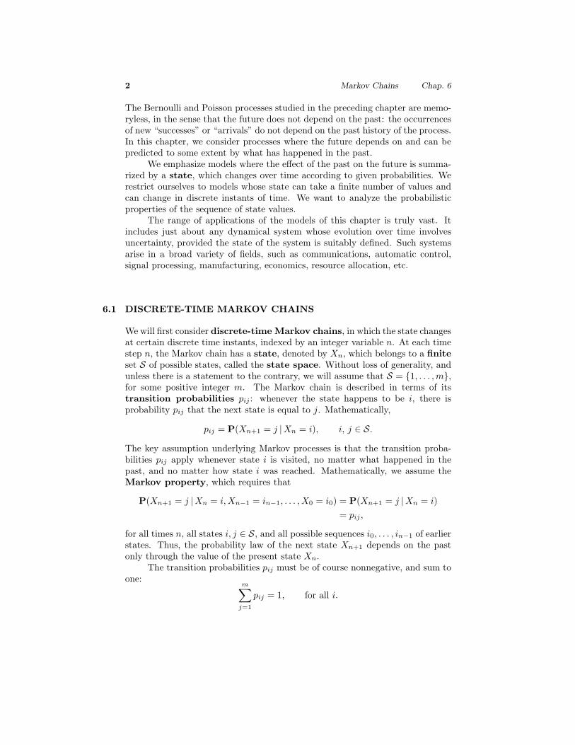
Example 6.1. Alice is taking a probability class and in each week she can beeither up-to-date or she may have fallen behind. If she is up-to-date in a givenweek, the probability that she will be up-to-date (or behind) in the next week is0.8 (or 0.2, respectively). If she is behind in the given week, the probability thatshe will be up-to-date (or behind) in the next week is 0.6 (or 0.4, respectively). Weassume that these probabilities do not depend on whether she was up-to-date orbehind in previous weeks, so the problem has the typical Markov chain character(the future depends on the past only through the present).
4 Markov Chains Chap. 6
Let us introduce states 1 and 2, and identify them with being up-to-date andbehind, respectively. Then, the transition probabilities are
p11 = 0.8, p12 = 0.2, p21 = 0.6, p22 = 0.4,
and the transition probability matrix is
[0.8 0.20.6 0.4
].
The transition probability graph is shown in Fig. 6.1.
1 2
Up-to-Date Behind
0.8
0.2
0.4
0.6
Figure 6.1: The transition probability graph in Example 6.1.
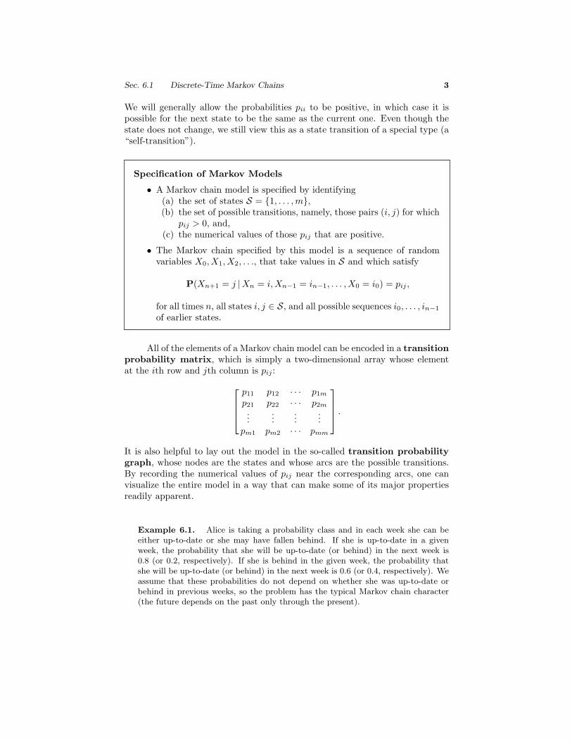
Example 6.2. A fly moves along a straight line in unit increments. At eachtime period, it moves one unit to the left with probability 0.3, one unit to the rightwith probability 0.3, and stays in place with probability 0.4, independently of thepast history of movements. A spider is lurking at positions 1 and m: if the flylands there, it is captured by the spider, and the process terminates. We want toconstruct a Markov chain model, assuming that the fly starts in one of the positions2, . . . , m − 1.
Let us introduce states 1, 2, . . . , m, and identify them with the correspondingpositions of the fly. The nonzero transition probabilities are
p11 = 1, pmm = 1,
pij ={
0.3 if j = i − 1 or j = i + 1,0.4 if j = i,
for i = 2, . . . , m − 1.
The transition probability graph and matrix are shown in Fig. 6.2.
Given a Markov chain model, we can compute the probability of any partic-ular sequence of future states. This is analogous to the use of the multiplicationrule in sequential (tree) probability models. In particular, we have
P(X0 = i0, X1 = i1, . . . , Xin = in) = P(X0 = i0)pi0i1pi1i2 · · · pin−1in .

Sec. 6.1 Discrete-Time Markov Chains 5
1 20.3
1
0.4
3 4 1
0.4
0.3
0.30.3
0.3
1
0.4
pij
3
2
4
1 32 4
1.0
1.0
000
0 000
0
0.40.3
0.30.3
Figure 6.2: The transition probability graph and the transition probability ma-trix in Example 6.2, for the case where m = 4.
To verify this property, note that
P(X0 = i0, X1 = i1, . . . , Xin = in)= P(Xn = in |X0 = i0, . . . , Xn−1 = in−1)P(X0 = i0, . . . , Xn−1 = in−1)= pin−1inP(X0 = i0, . . . , Xn−1 = in−1),
where the last equality made use of the Markov property. We then apply thesame argument to the term P(X0 = i0, . . . , Xn−1 = in−1) and continue similarly,until we eventually obtain the desired expression. If the initial state X0 is givenand is known to be equal to some i0, a similar argument yields
P(X1 = i1, . . . , Xin = in |X0 = i0) = pi0i1pi1i2 · · · pin−1in .
Graphically, a state sequence can be identified with a sequence of arcs in thetransition probability graph, and the probability of such a path (given the ini-tial state) is given by the product of the probabilities associated with the arcstraversed by the path.
Example 6.3. For the spider and fly example (Example 6.2), we have
P(X1 = 2, X2 = 2, X3 = 3, X4 = 4 |X0 = 2) = p22p22p23p34 = (0.4)2(0.3)2.
We also have
P(X0 = 2, X1 = 2, X2 = 2, X3 = 3, X4 = 4) = P(X0 = 2)p22p22p23p34
= P(X0 = 2)(0.4)2(0.3)2.
Note that in order to calculate a probability of this form, in which there is noconditioning on a fixed initial state, we need to specify a probability law for theinitial state X0.

6 Markov Chains Chap. 6
n-Step Transition Probabilities
Many Markov chain problems require the calculation of the probability law ofthe state at some future time, conditioned on the current state. This probabilitylaw is captured by the n-step transition probabilities, defined by
rij(n) = P(Xn = j |X0 = i).
In words, rij(n) is the probability that the state after n time periods will be j,given that the current state is i. It can be calculated using the following basicrecursion, known as the Chapman-Kolmogorov equation.
Chapman-Kolmogorov Equation for the n-Step TransitionProbabilities
The n-step transition probabilities can be generated by the recursive formula
rij(n) =m∑
k=1
rik(n − 1)pkj , for n > 1, and all i, j,
starting withrij(1) = pij .
To verify the formula, we apply the total probability theorem as follows:
P(Xn = j |X0 = i) =m∑
k=1
P(Xn−1 = k |X0 = i) · P(Xn = j |Xn−1 = k, X0 = i)
=m∑
k=1
rik(n − 1)pkj ;
see Fig. 6.3 for an illustration. We have used here the Markov property: oncewe condition on Xn−1 = k, the conditioning on X0 = i does not affect theprobability pkj of reaching j at the next step.
We can view rij(n) as the element at the ith row and jth column of a two-dimensional array, called the n-step transition probability matrix.† Figures
† Those readers familiar with matrix multiplication, may recognize that theChapman-Kolmogorov equation can be expressed as follows: the matrix of n-step tran-sition probabilities rij(n) is obtained by multiplying the matrix of (n − 1)-step tran-sition probabilities rik(n − 1), with the one-step transition probability matrix. Thus,the n-step transition probability matrix is the nth power of the transition probabilitymatrix.

Sec. 6.1 Discrete-Time Markov Chains 7
1
k
j
m
...
pmj
p1j
i
ri1(n-1)
rik(n-1)
rim(n-1)
...
pkj
Time 0 Time n-1 Time n
Figure 6.3: Derivation of the Chapman-Kolmogorov equation. The probabilityof being at state j at time n is the sum of the probabilities rik(n − 1)pkj of thedifferent ways of reaching j.
BUpD
B
UpD 0.8 0.2
0.40.6
.76 .24
.28.72
.752 .248
.256.744
.7504 .2496
.2512.7488
rij (5)
.7501 .2499
.2502.7498
rij (1) rij (2) rij (3) rij (4)
Sequence of n -step transition probability matrices
n-step transition probabilities as a function of the numbern of transitions
0
0.75
0.25
n
r11(n)
r12(n)
0
0.75
0.25
n
r22(n)r21(n)
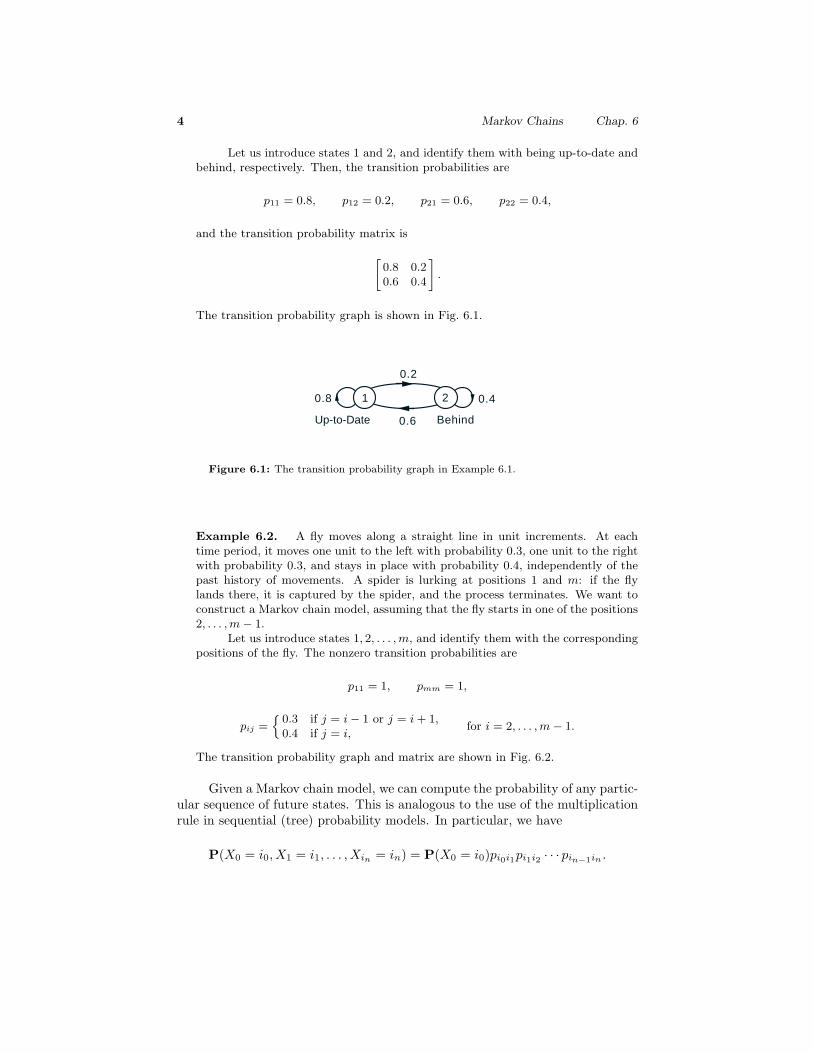
Figure 6.4: n-step transition probabilities for the “up-to-date/behind” Example6.1. Observe that as n → ∞, rij(n) converges to a limit that does not depend onthe initial state.
6.4 and 6.5 give the n-step transition probabilities rij(n) for the cases of Ex-amples 6.1 and 6.2, respectively. There are some interesting observations aboutthe limiting behavior of rij(n) in these two examples. In Fig. 6.4, we see that

8 Markov Chains Chap. 6
each rij(n) converges to a limit, as n → ∞, and this limit does not depend onthe initial state. Thus, each state has a positive “steady-state” probability ofbeing occupied at times far into the future. Furthermore, the probability rij(n)depends on the initial state i when n is small, but over time this dependencediminishes. Many (but by no means all) probabilistic models that evolve overtime have such a character: after a sufficiently long time, the effect of their initialcondition becomes negligible.
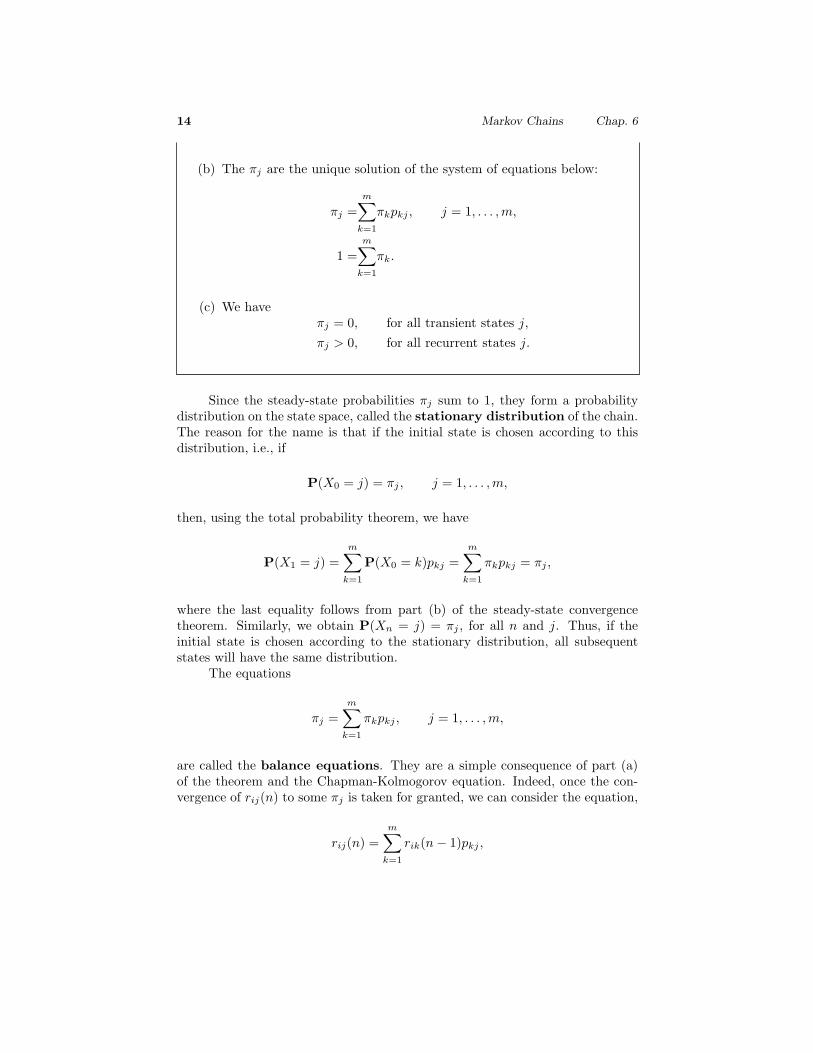
In Fig. 6.5, we see a qualitatively different behavior: rij(n) again converges,but the limit depends on the initial state, and can be zero for selected states.Here, we have two states that are “absorbing,” in the sense that they are infinitelyrepeated, once reached. These are the states 1 and 4 that correspond to thecapture of the fly by one of the two spiders. Given enough time, it is certainthat some absorbing state will be reached. Accordingly, the probability of beingat the non-absorbing states 2 and 3 diminishes to zero as time increases.
1
3
2
4
1 32 4
0.3
0.4
1.0
1.0
000
0 000
0
0.40.3
0.30.3 .25
1.0
1.0
000
0 00
.09.24.42 .17
1.0
1.0
000
0 00
.16.17.50 .12
1.0
1.0
000
0 00
.21.12.55 0
1.0
1.0
000
0 00
1/302/3
rij (1) rij (2) rij (3) rij (4) rij (∞)
.09 .24 .42.25 .17.16 .17 .50 .12.21 .12 .55. . . .
01/3 0 2/3
Sequence of transition probability matrices
n-step transition probabilities as a function of the time n
0 n
r21(n)
r24(n)
2/3
1/3r22(n)
r23(n)
Figure 6.5: n-step transition probabilities for the “spiders-and-fly” Example 6.2.Observe that rij(n) converges to a limit that depends on the initial state.
These examples illustrate that there is a variety of types of states andasymptotic occupancy behavior in Markov chains. We are thus motivated toclassify and analyze the various possibilities, and this is the subject of the nextthree sections.

Sec. 6.2 Classification of States 9
6.2 CLASSIFICATION OF STATES
In the preceding section, we saw through examples several types of Markov chainstates with qualitatively different characteristics. In particular, some states, afterbeing visited once, are certain to be revisited again, while for some other statesthis may not be the case. In this section, we focus on the mechanism by whichthis occurs. In particular, we wish to classify the states of a Markov chain witha focus on the long-term frequency with which they are visited.
As a first step, we make the notion of revisiting a state precise. Let us saythat a state j is accessible from a state i if for some n, the n-step transitionprobability rij(n) is positive, i.e., if there is positive probability of reaching j,starting from i, after some number of time periods. An equivalent definition isthat there is a possible state sequence i, i1, . . . , in−1, j, that starts at i and endsat j, in which the transitions (i, i1), (i1, i2), . . . , (in−2, in−1), (in−1, j) all havepositive probability. Let A(i) be the set of states that are accessible from i. Wesay that i is recurrent if for every j that is accessible from i, i is also accessiblefrom j; that is, for all j that belong to A(i) we have that i belongs to A(j).
When we start at a recurrent state i, we can only visit states j ∈ A(i)from which i is accessible. Thus, from any future state, there is always someprobability of returning to i and, given enough time, this is certain to happen.By repeating this argument, if a recurrent state is visited once, it will be revisitedan infinite number of times.
A state is called transient if it is not recurrent. In particular, there arestates j ∈ A(i) such that i is not accessible from j. After each visit to state i,there is positive probability that the state enters such a j. Given enough time,this will happen, and state i cannot be visited after that. Thus, a transient statewill only be visited a finite number of times.
Note that transience or recurrence is determined by the arcs of the tran-sition probability graph [those pairs (i, j) for which pij > 0] and not by thenumerical values of the pij . Figure 6.6 provides an example of a transition prob-ability graph, and the corresponding recurrent and transient states.
1 2 3 4
Recurrent RecurrentRecurrentTransient
Figure 6.6: Classification of states given the transition probability graph. Start-ing from state 1, the only accessible state is itself, and so 1 is a recurrent state.States 1, 3, and 4 are accessible from 2, but 2 is not accessible from any of them,so state 2 is transient. States 3 and 4 are accessible only from each other (andthemselves), and they are both recurrent.
If i is a recurrent state, the set of states A(i) that are accessible from i

10 Markov Chains Chap. 6
form a recurrent class (or simply class), meaning that states in A(i) are allaccessible from each other, and no state outside A(i) is accessible from them.Mathematically, for a recurrent state i, we have A(i) = A(j) for all j that belongto A(i), as can be seen from the definition of recurrence. For example, in thegraph of Fig. 6.6, states 3 and 4 form a class, and state 1 by itself also forms aclass.
It can be seen that at least one recurrent state must be accessible from anygiven transient state. This is intuitively evident, and a more precise justificationis given in the theoretical problems section. It follows that there must existat least one recurrent state, and hence at least one class. Thus, we reach thefollowing conclusion.
Markov Chain Decomposition
• A Markov chain can be decomposed into one or more recurrent classes,plus possibly some transient states.
• A recurrent state is accessible from all states in its class, but is notaccessible from recurrent states in other classes.
• A transient state is not accessible from any recurrent state.
• At least one, possibly more, recurrent states are accessible from a giventransient state.
Figure 6.7 provides examples of Markov chain decompositions. Decompo-sition provides a powerful conceptual tool for reasoning about Markov chainsand visualizing the evolution of their state. In particular, we see that:
(a) once the state enters (or starts in) a class of recurrent states, it stays withinthat class; since all states in the class are accessible from each other, allstates in the class will be visited an infinite number of times;
(b) if the initial state is transient, then the state trajectory contains an ini-tial portion consisting of transient states and a final portion consisting ofrecurrent states from the same class.
For the purpose of understanding long-term behavior of Markov chains, it is im-portant to analyze chains that consist of a single recurrent class. For the purposeof understanding short-term behavior, it is also important to analyze the mech-anism by which any particular class of recurrent states is entered starting from agiven transient state. These two issues, long-term and short-term behavior, arethe focus of Sections 6.3 and 6.4, respectively.
Periodicity
One more characterization of a recurrent class is of special interest, and relates

Sec. 6.2 Classification of States 11
1 2 3 4
Single class of recurrent states
1 2
3
Single class of recurrent states (1 and 2)and one transient state (3)
Two classes of recurrent states (class of state1 and class of states 4 and 5)and two transient states (2 and 3)
1 2 3 4 5
Figure 6.7: Examples of Markov chain decompositions into recurrent classes andtransient states.
to the presence or absence of a certain periodic pattern in the times that a stateis visited. In particular, a recurrent class is said to be periodic if its states canbe grouped in d > 1 disjoint subsets S1, . . . , Sd so that all transitions from onesubset lead to the next subset; see Fig. 6.8. More precisely,
if i ∈ Sk and pij > 0, then{
j ∈ Sk+1, if k = 1, . . . , d − 1,j ∈ S1, if k = d.
A recurrent class that is not periodic, is said to be aperiodic.Thus, in a periodic recurrent class, we move through the sequence of subsets
in order, and after d steps, we end up in the same subset. As an example, therecurrent class in the second chain of Fig. 6.7 (states 1 and 2) is periodic, andthe same is true of the class consisting of states 4 and 5 in the third chain of Fig.6.7. All other classes in the chains of this figure are aperiodic.

12 Markov Chains Chap. 6
6
1
2
3
4
5
S1
S3
S2
Figure 6.8: Structure of a periodic recurrent class.
Note that given a periodic recurrent class, a positive time n, and a state j inthe class, there must exist some state i such that rij(n) = 0. The reason is that,from the definition of periodicity, the states are grouped in subsets S1, . . . , Sd,and the subset to which j belongs can be reached at time n from the states inonly one of the subsets. Thus, a way to verify aperiodicity of a given recurrentclass R, is to check whether there is a special time n ≥ 1 and a special states ∈ R that can be reached at time n from all initial states in R, i.e., ris(n) > 0for all i ∈ R. As an example, consider the first chain in Fig. 6.7. State s = 2can be reached at time n = 2 starting from every state, so the unique recurrentclass of that chain is aperiodic.
A converse statement, which we do not prove, also turns out to be true:if a recurrent class is not periodic, then a time n and a special state s with theabove properties can always be found.
Periodicity
Consider a recurrent class R.
• The class is called periodic if its states can be grouped in d > 1disjoint subsets S1, . . . , Sd, so that all transitions from Sk lead to Sk+1
(or to S1 if k = d).
• The class is aperiodic (not periodic) if and only if there exists a timen and a state s in the class, such that pis(n) > 0 for all i ∈ R.

Sec. 6.3 Steady-State Behavior 13
6.3 STEADY-STATE BEHAVIOR
In Markov chain models, we are often interested in long-term state occupancybehavior, that is, in the n-step transition probabilities rij(n) when n is verylarge. We have seen in the example of Fig. 6.4 that the rij(n) may converge tosteady-state values that are independent of the initial state, so to what extentis this behavior typical?
If there are two or more classes of recurrent states, it is clear that thelimiting values of the rij(n) must depend on the initial state (visiting j far intothe future will depend on whether j is in the same class as the initial state i).We will, therefore, restrict attention to chains involving a single recurrent class,plus possibly some transient states. This is not as restrictive as it may seem,since we know that once the state enters a particular recurrent class, it will staywithin that class. Thus, asymptotically, the presence of all classes except for oneis immaterial.
Even for chains with a single recurrent class, the rij(n) may fail to converge.To see this, consider a recurrent class with two states, 1 and 2, such that fromstate 1 we can only go to 2, and from 2 we can only go to 1 (p12 = p21 = 1).Then, starting at some state, we will be in that same state after any even numberof transitions, and in the other state after any odd number of transitions. Whatis happening here is that the recurrent class is periodic, and for such a class, itcan be seen that the rij(n) generically oscillate.
We now assert that for every state j, the n-step transition probabilitiesrij(n) approach a limiting value that is independent of i, provided we excludethe two situations discussed above (multiple recurrent classes and/or a periodicclass). This limiting value, denoted by πj , has the interpretation
πj ≈ P(Xn = j), when n is large,
and is called the steady-state probability of j. The following is an importanttheorem. Its proof is quite complicated and is outlined together with severalother proofs in the theoretical problems section.
Steady-State Convergence Theorem
Consider a Markov chain with a single recurrent class, which is aperiodic.Then, the states j are associated with steady-state probabilities πj thathave the following properties.
(a) limn→∞
rij(n) = πj , for all i, j.
14 Markov Chains Chap. 6
(b) The πj are the unique solution of the system of equations below:
πj =m∑
k=1
πkpkj , j = 1, . . . , m,
1 =m∑
k=1
πk.
(c) We haveπj = 0, for all transient states j,
πj > 0, for all recurrent states j.
Since the steady-state probabilities πj sum to 1, they form a probabilitydistribution on the state space, called the stationary distribution of the chain.The reason for the name is that if the initial state is chosen according to thisdistribution, i.e., if
P(X0 = j) = πj , j = 1, . . . , m,
then, using the total probability theorem, we have
P(X1 = j) =m∑
k=1
P(X0 = k)pkj =m∑
k=1
πkpkj = πj ,
where the last equality follows from part (b) of the steady-state convergencetheorem. Similarly, we obtain P(Xn = j) = πj , for all n and j. Thus, if theinitial state is chosen according to the stationary distribution, all subsequentstates will have the same distribution.
The equations
πj =m∑
k=1
πkpkj , j = 1, . . . , m,
are called the balance equations. They are a simple consequence of part (a)of the theorem and the Chapman-Kolmogorov equation. Indeed, once the con-vergence of rij(n) to some πj is taken for granted, we can consider the equation,
rij(n) =m∑
k=1
rik(n − 1)pkj ,

Sec. 6.3 Steady-State Behavior 15
take the limit of both sides as n → ∞, and recover the balance equations.† Thebalance equations are a linear system of equations that, together with
∑mk=1 πk =
1, can be solved to obtain the πj . The following examples illustrate the solutionprocess.
Example 6.4. Consider a two-state Markov chain with transition probabilities
p11 = 0.8, p12 = 0.2,
p21 = 0.6, p22 = 0.4.
[This is the same as the chain of Example 6.1 (cf. Fig. 6.1).] The balance equationstake the form
π1 = π1p11 + π2p21, π2 = π1p12 + π2p22,
orπ1 = 0.8 · π1 + 0.6 · π2, π2 = 0.2 · π1 + 0.4 · π2.
Note that the above two equations are dependent, since they are both equivalentto
π1 = 3π2.
This is a generic property, and in fact it can be shown that one of the balance equa-tions depends on the remaining equations (see the theoretical problems). However,we know that the πj satisfy the normalization equation
π1 + π2 = 1,
which supplements the balance equations and suffices to determine the πj uniquely.Indeed, by substituting the equation π1 = 3π2 into the equation π1 + π2 = 1, weobtain 3π2 + π2 = 1, or
π2 = 0.25,
which using the equation π1 + π2 = 1, yields
π1 = 0.75.
This is consistent with what we found earlier by iterating the Chapman-Kolmogorovequation (cf. Fig. 6.4).
Example 6.5. An absent-minded professor has two umbrellas that she uses whencommuting from home to office and back. If it rains and an umbrella is available in
† According to a famous and important theorem from linear algebra (called thePerron-Frobenius theorem), the balance equations always have a nonnegative solution,for any Markov chain. What is special about a chain that has a single recurrent class,which is aperiodic, is that the solution is unique and is also equal to the limit of then-step transition probabilities rij(n).
16 Markov Chains Chap. 6
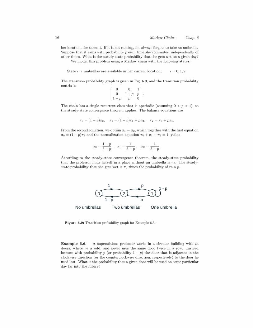
her location, she takes it. If it is not raining, she always forgets to take an umbrella.Suppose that it rains with probability p each time she commutes, independently ofother times. What is the steady-state probability that she gets wet on a given day?
We model this problem using a Markov chain with the following states:
State i: i umbrellas are available in her current location, i = 0, 1, 2.
The transition probability graph is given in Fig. 6.9, and the transition probabilitymatrix is [
0 0 10 1 − p p
1 − p p 0
].
The chain has a single recurrent class that is aperiodic (assuming 0 < p < 1), sothe steady-state convergence theorem applies. The balance equations are
π0 = (1 − p)π2, π1 = (1 − p)π1 + pπ2, π2 = π0 + pπ1.
From the second equation, we obtain π1 = π2, which together with the first equationπ0 = (1 − p)π2 and the normalization equation π0 + π1 + π2 = 1, yields
π0 =1 − p
3 − p, π1 =
1
3 − p, π2 =
1
3 − p.
According to the steady-state convergence theorem, the steady-state probabilitythat the professor finds herself in a place without an umbrella is π0. The steady-state probability that she gets wet is π0 times the probability of rain p.
120
1
1 - p
1 - pp
p
No umbrellas Two umbrellas One umbrella
Figure 6.9: Transition probability graph for Example 6.5.
Example 6.6. A superstitious professor works in a circular building with mdoors, where m is odd, and never uses the same door twice in a row. Insteadhe uses with probability p (or probability 1 − p) the door that is adjacent in theclockwise direction (or the counterclockwise direction, respectively) to the door heused last. What is the probability that a given door will be used on some particularday far into the future?

Sec. 6.3 Steady-State Behavior 17
1 2
3
p 1 - p
1 - p
1 - p
1 - p p
p
p
Door 1
Door 3
Door 4
Door 2
5
4
Door 5 1 - p
p
Figure 6.10: Transition probability graph in Example 6.6, for the case ofm = 5 doors.
We introduce a Markov chain with the following m states:
State i: Last door used is door i, i = 1, . . . , m.
The transition probability graph of the chain is given in Fig. 6.10, for the casem = 5. The transition probability matrix is
0 p 0 0 . . . 0 1 − p
1 − p 0 p 0 . . . 0 00 1 − p 0 p . . . 0 0...
......
......
......
p 0 0 0 . . . 1 − p 0
.
Assuming that 0 < p < 1, the chain has a single recurrent class that is aperiodic.[To verify aperiodicity, argue by contradiction: if the class were periodic, therecould be only two subsets of states such that transitions from one subset lead tothe other, since it is possible to return to the starting state in two transitions. Thus,it cannot be possible to reach a state i from a state j in both an odd and an evennumber of transitions. However, if m is odd, this is true for states 1 and m – acontradiction (for example, see the case where m = 5 in Fig. 6.10, doors 1 and 5 canbe reached from each other in 1 transition and also in 4 transitions).] The balanceequations are
π1 = (1 − p)π2 + pπm,
πi = pπi−1 + (1 − p)πi+1, i = 2, . . . , m − 1,
πm = (1 − p)π1 + pπm−1.
These equations are easily solved once we observe that by symmetry, all doorsshould have the same steady-state probability. This suggests the solution
πj =1
m, j = 1, . . . , m.
18 Markov Chains Chap. 6
Indeed, we see that these πj satisfy the balance equations as well as the normal-ization equation, so they must be the desired steady-state probabilities (by theuniquenes part of the steady-state convergence theorem).
Note that if either p = 0 or p = 1, the chain still has a single recurrentclass but is periodic. In this case, the n-step transition probabilities rij(n) do notconverge to a limit, because the doors are used in a cyclic order. Similarly, if m iseven, the recurrent class of the chain is periodic, since the states can be groupedinto two subsets, the even and the odd numbered states, such that from each subsetone can only go to the other subset.
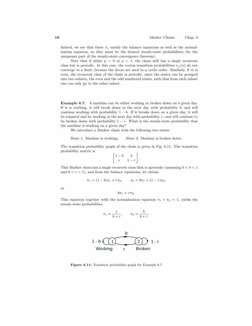
Example 6.7. A machine can be either working or broken down on a given day.If it is working, it will break down in the next day with probability b, and willcontinue working with probability 1 − b. If it breaks down on a given day, it willbe repaired and be working in the next day with probability r, and will continue tobe broken down with probability 1 − r. What is the steady-state probability thatthe machine is working on a given day?
We introduce a Markov chain with the following two states:
State 1: Machine is working, State 2: Machine is broken down.
The transition probability graph of the chain is given in Fig. 6.11. The transitionprobability matrix is [
1 − b br 1 − r
].
This Markov chain has a single recurrent class that is aperiodic (assuming 0 < b < 1and 0 < r < 1), and from the balance equations, we obtain
π1 = (1 − b)π1 + rπ2, π2 = bπ1 + (1 − r)π2,
orbπ1 = rπ2.
This equation together with the normalization equation π1 + π2 = 1, yields thesteady-state probabilities
π1 =r
b + r, π2 =
b
b + r.
1 2
Working Broken
1 - b
r
b
1 - r
Figure 6.11: Transition probability graph for Example 6.7.
Sec. 6.3 Steady-State Behavior 19
The situation considered in the previous example has evidently the Markovproperty, i.e., the state of the machine at the next day depends explicitly only onits state at the present day. However, it is possible to use a Markov chain modeleven if there is a dependence on the states at several past days. The generalidea is to introduce some additional states which encode what has happened inpreceding periods. Here is an illustration of this technique.
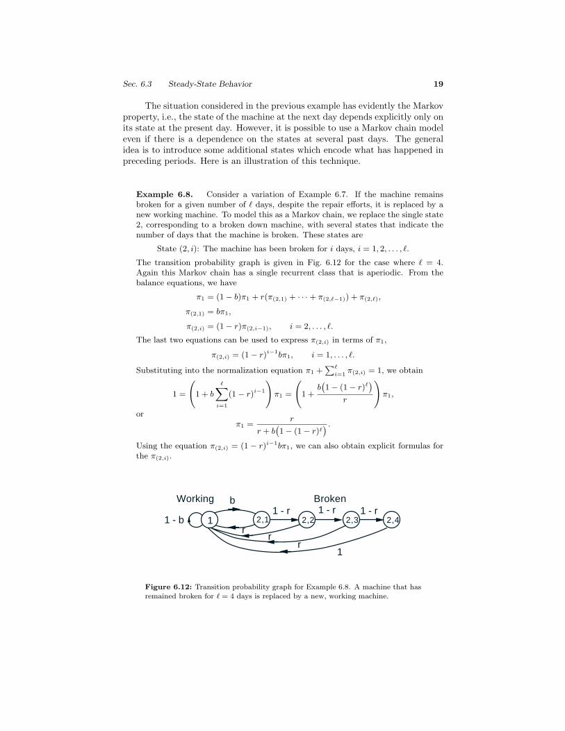
Example 6.8. Consider a variation of Example 6.7. If the machine remainsbroken for a given number of � days, despite the repair efforts, it is replaced by anew working machine. To model this as a Markov chain, we replace the single state2, corresponding to a broken down machine, with several states that indicate thenumber of days that the machine is broken. These states are
State (2, i): The machine has been broken for i days, i = 1, 2, . . . , �.
The transition probability graph is given in Fig. 6.12 for the case where � = 4.Again this Markov chain has a single recurrent class that is aperiodic. From thebalance equations, we have
π1 = (1 − b)π1 + r(π(2,1) + · · · + π(2,�−1)) + π(2,�),
π(2,1) = bπ1,
π(2,i) = (1 − r)π(2,i−1), i = 2, . . . , �.
The last two equations can be used to express π(2,i) in terms of π1,
π(2,i) = (1 − r)i−1bπ1, i = 1, . . . , �.
Substituting into the normalization equation π1 +∑�
i=1π(2,i) = 1, we obtain
1 =
(1 + b
�∑i=1
(1 − r)i−1
)π1 =
(1 +
b(1 − (1 − r)�
)r
)π1,
orπ1 =
r
r + b(1 − (1 − r)�
) .
Using the equation π(2,i) = (1 − r)i−1bπ1, we can also obtain explicit formulas forthe π(2,i).
1 2,1
Working Broken
1 - br
b1 - r
2,2 2,3 2,41 - r 1 - r
rr
1
Figure 6.12: Transition probability graph for Example 6.8. A machine that hasremained broken for � = 4 days is replaced by a new, working machine.

20 Markov Chains Chap. 6
Long-Term Frequency Interpretations
Probabilities are often interpreted as relative frequencies in an infinitely longstring of independent trials. The steady-state probabilities of a Markov chainadmit a similar interpretation, despite the absence of independence.
Consider, for example, a Markov chain involving a machine, which at theend of any day can be in one of two states, working or broken-down. Each time itbreaks down, it is immediately repaired at a cost of $1. How are we to model thelong-term expected cost of repair per day? One possibility is to view it as theexpected value of the repair cost on a randomly chosen day far into the future;this is just the steady-state probability of the broken down state. Alternatively,we can calculate the total expected repair cost in n days, where n is very large,and divide it by n. Intuition suggests that these two methods of calculationshould give the same result. Theory supports this intuition, and in general wehave the following interpretation of steady-state probabilities (a justification isgiven in the theoretical problems section).
Steady-State Probabilities as Expected State Frequencies
For a Markov chain with a single class that is aperiodic, the steady-stateprobabilities πj satisfy
πj = limn→∞
vij(n)n
,
where vij(n) is the expected value of the number of visits to state j withinthe first n transitions, starting from state i.
Based on this interpretation, πj is the long-term expected fraction of timethat the state is equal to j. Each time that state j is visited, there is probabilitypjk that the next transition takes us to state k. We conclude that πjpjk canbe viewed as the long-term expected fraction of transitions that move the statefrom j to k.†
† In fact, some stronger statements are also true. Namely, whenever we carryout the probabilistic experiment and generate a trajectory of the Markov chain overan infinite time horizon, the observed long-term frequency with which state j is visitedwill be exactly equal to πj , and the observed long-term frequency of transitions fromj to k will be exactly equal to πjpjk. Even though the trajectory is random, theseequalities hold with certainty, that is, with probability 1. The exact meaning of thisstatement will become more apparent in the next chapter, when we discuss conceptsrelated to the limiting behavior of random processes.

Sec. 6.3 Steady-State Behavior 21
Expected Frequency of a Particular Transition
Consider n transitions of a Markov chain with a single class that is aperiodic,starting from a given initial state. Let qjk(n) be the expected number ofsuch transitions that take the state from j to k. Then, regardless of theinitial state, we have
limn→∞
qjk(n)n
= πjpjk.
The frequency interpretation of πj and πjpjk allows for a simple interpre-tation of the balance equations. The state is equal to j if and only if there is atransition that brings the state to j. Thus, the expected frequency πj of visits toj is equal to the sum of the expected frequencies πkpkj of transitions that leadto j, and
πj =m∑
k=1
πkpkj ;
see Fig. 6.13.
1
2
j
m
... ...
π1p1j
p2j
pmjπm
π2
pj j π j
Figure 6.13: Interpretation of the balance equations in terms of frequencies.In a very large number of transitions, there will be a fraction πkpkj that bringthe state from k to j. (This also applies to transitions from j to itself, whichoccur with frequency πjpjj .) The sum of the frequencies of such transitions is thefrequency πj of being at state j.
Birth-Death Processes
A birth-death process is a Markov chain in which the states are linearly ar-ranged and transitions can only occur to a neighboring state, or else leave thestate unchanged. They arise in many contexts, especially in queueing theory.

22 Markov Chains Chap. 6
Figure 6.14 shows the general structure of a birth-death process and also intro-duces some generic notation for the transition probabilities. In particular,
bi = P(Xn+1 = i + 1 |Xn = i), (“birth” probability at state i),di = P(Xn+1 = i − 1 |Xn = i), (“death” probability at state i).
. . . m - 1 m
1 - dm
bm-2
0 1
b0
d1
1 - b1 - d11 - b0
b1
d2 dm-1
1 - bm-1 - dm-1
bm-1
dm
Figure 6.14: Transition probability graph for a birth-death process.
For a birth-death process, the balance equations can be substantially sim-plified. Let us focus on two neighboring states, say, i and i+1. In any trajectoryof the Markov chain, a transition from i to i+1 has to be followed by a transitionfrom i + 1 to i, before another transition from i to i + 1 can occur. Therefore,the frequency of transitions from i to i + 1, which is πibi, must be equal to thefrequency of transitions from i + 1 to i, which is πi+1di+1. This leads to thelocal balance equations†
πibi = πi+1di+1, i = 0, 1, . . . , m − 1.
Using the local balance equations, we obtain
πi = π0b0b1 · · · bi−1
d1d2 · · · di, i = 1, . . . , m.
Together with the normalization equation∑
i πi = 1, the steady-state probabil-ities πi are easily computed.
Example 6.9. (Random Walk with Reflecting Barriers) A person walksalong a straight line and, at each time period, takes a step to the right with prob-ability b, and a step to the left with probability 1 − b. The person starts in one of
† A more formal derivation that does not rely on the frequency interpretationproceeds as follows. The balance equation at state 0 is π0(1 − b0) + π1d1 = π0, whichyields the first local balance equation π0b0 = π1d1.
The balance equation at state 1 is π0b0 + π1(1 − b1 − d1) + π2d2 = π1. Usingthe local balance equation π0b0 = π1d1 at the previous state, this is rewritten asπ1d1 + π1(1 − b1 − d1) + π2d2 = π1, which simplifies to π1b1 = π2d2. We can thencontinue similarly to obtain the local balance states at all other states.
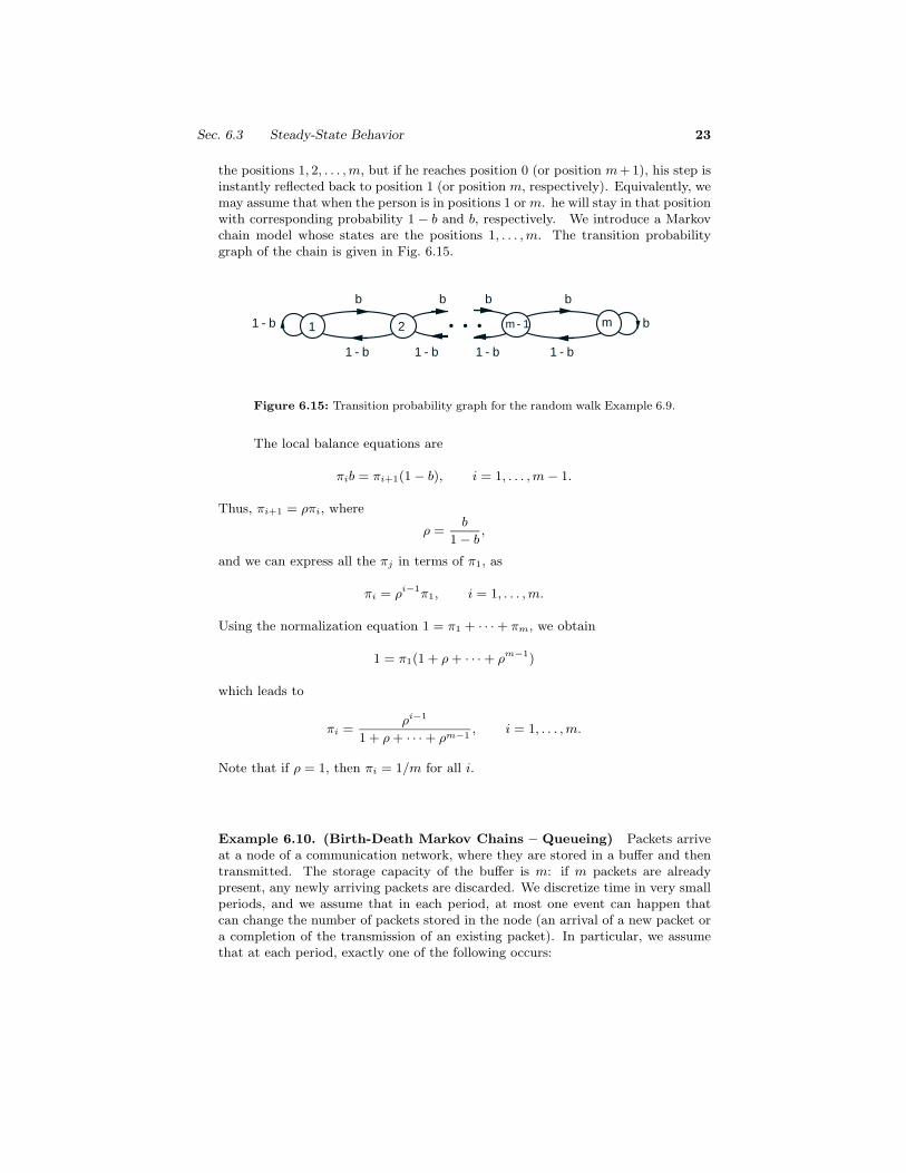
Sec. 6.3 Steady-State Behavior 23
the positions 1, 2, . . . , m, but if he reaches position 0 (or position m+1), his step isinstantly reflected back to position 1 (or position m, respectively). Equivalently, wemay assume that when the person is in positions 1 or m. he will stay in that positionwith corresponding probability 1 − b and b, respectively. We introduce a Markovchain model whose states are the positions 1, . . . , m. The transition probabilitygraph of the chain is given in Fig. 6.15.
21 . . . m - 1 m
b
1 - b
bb b
1 - b 1 - b 1 - b
1 - b b
Figure 6.15: Transition probability graph for the random walk Example 6.9.
The local balance equations are
πib = πi+1(1 − b), i = 1, . . . , m − 1.
Thus, πi+1 = ρπi, where
ρ =b
1 − b,
and we can express all the πj in terms of π1, as
πi = ρi−1π1, i = 1, . . . , m.
Using the normalization equation 1 = π1 + · · · + πm, we obtain
1 = π1(1 + ρ + · · · + ρm−1)
which leads to
πi =ρi−1
1 + ρ + · · · + ρm−1, i = 1, . . . , m.
Note that if ρ = 1, then πi = 1/m for all i.
Example 6.10. (Birth-Death Markov Chains – Queueing) Packets arriveat a node of a communication network, where they are stored in a buffer and thentransmitted. The storage capacity of the buffer is m: if m packets are alreadypresent, any newly arriving packets are discarded. We discretize time in very smallperiods, and we assume that in each period, at most one event can happen thatcan change the number of packets stored in the node (an arrival of a new packet ora completion of the transmission of an existing packet). In particular, we assumethat at each period, exactly one of the following occurs:

24 Markov Chains Chap. 6
(a) one new packet arrives; this happens with a given probability b > 0;
(b) one existing packet completes transmission; this happens with a given prob-ability d > 0 if there is at least one packet in the node, and with probability0 otherwise;
(c) no new packet arrives and no existing packet completes transmission; thishappens with a probability 1−b−d if there is at least one packet in the node,and with probability 1 − b otherwise.
We introduce a Markov chain with states 0, 1, . . . , m, corresponding to thenumber of packets in the buffer. The transition probability graph is given inFig. 6.16.
The local balance equations are
πib = πi+1d, i = 0, 1, . . . , m − 1.
We define
ρ =b
d,
and obtain πi+1 = ρπi, which leads to πi = ρiπ0 for all i. By using the normalizationequation 1 = π0 + π1 + · · · + πm, we obtain
1 = π0(1 + ρ + · · · + ρm),
and
π0 =
1 − ρ
1 − ρm+1if ρ �= 1,
1
m + 1if ρ = 1.
The steady-state probabilities are then given by
πi =
ρi(1 − ρ)
1 − ρm+1if ρ �= 1,
1
m + 1if ρ = 1,
i = 0, 1, . . . , m.
0 1 . . . m - 1 m
b
d
1 - b - d1 - b 1 - d
bb b
d d d
1 - b - d
Figure 6.16: Transition probability graph in Example 6.10.

Sec. 6.4 Absorption Probabilities and Expected Time to Absorption 25
It is interesting to consider what happens when the buffer size m is so largethat it can be considered as practically infinite. We distinguish two cases.
(a) Suppose that b < d, or ρ < 1. In this case, arrivals of new packets areless likely than departures of existing packets. This prevents the numberof packets in the buffer from growing, and the steady-state probabilities πi
decrease with i. We observe that as m → ∞, we have 1 − ρm+1 → 1, and
πi → ρi(1 − ρ), for all i.
We can view these as the steady-state probabilities in a system with an infinitebuffer. [As a check, note that we have
∑∞i=0
ρi(1 − ρ) = 1.]
(b) Suppose that b > d, or ρ > 1. In this case, arrivals of new packets are morelikely than departures of existing packets. The number of packets in the buffertends to increase, and the steady-state probabilities πi increase with i. As weconsider larger and larger buffer sizes m, the steady-state probability of anyfixed state i decreases to zero:
πi → 0, for all i.
Were we to consider a system with an infinite buffer, we would have a Markovchain with a countably infinite number of states. Although we do not havethe machinery to study such chains, the preceding calculation suggests thatevery state will have zero steady-state probability and will be “transient.” Thenumber of packets in queue will generally grow to infinity, and any particularstate will be visited only a finite number of times.
6.4 ABSORPTION PROBABILITIES AND EXPECTED TIMETO ABSORPTION
In this section, we study the short-term behavior of Markov chains. We firstconsider the case where the Markov chain starts at a transient state. We areinterested in the first recurrent state to be entered, as well as in the time untilthis happens.
When focusing on such questions, the subsequent behavior of the Markovchain (after a recurrent state is encountered) is immaterial. We can thereforeassume, without loss of generality, that every recurrent state k is absorbing,i.e.,
pkk = 1, pkj = 0 for all j �= k.
If there is a unique absorbing state k, its steady-state probability is 1 (becauseall other states are transient and have zero steady-state probability), and will bereached with probability 1, starting from any initial state. If there are multipleabsorbing states, the probability that one of them will be eventually reached isstill 1, but the identity of the absorbing state to be entered is random and the
26 Markov Chains Chap. 6
associated probabilities may depend on the starting state. In the sequel, we fix aparticular absorbing state, denoted by s, and consider the absorption probabilityai that s is eventually reached, starting from i:
ai = P(Xn eventually becomes equal to the absorbing state s |X0 = i).
Absorption probabilities can be obtained by solving a system of linear equations,as indicated below.
Absorption Probability Equations
Consider a Markov chain in which each state is either transient or absorbing.We fix a particular absorbing state s. Then, the probabilities ai of eventuallyreaching state s, starting from i, are the unique solution of the equations
as = 1,
ai = 0, for all absorbing i �= s,
ai =m∑
j=1
pijaj , for all transient i.
The equations as = 1, and ai = 0, for all absorbing i �= s, are evidentfrom the definitions. To verify the remaining equations, we argue as follows. Letus consider a transient state i and let A be the event that state s is eventuallyreached. We haveai = P(A |X0 = i)
=m∑
j=1
P(A |X0 = i, X1 = j)P(X1 = j |X0 = i) (total probability thm.)
=m∑
j=1
P(A |X1 = j)pij (Markov property)
=m∑
j=1
ajpij .
The uniqueness property of the solution of the absorption probability equationsrequires a separate argument, which is given in the theoretical problems section.
The next example illustrates how we can use the preceding method tocalculate the probability of entering a given recurrent class (rather than a givenabsorbing state).
Example 6.11. Consider the Markov chain shown in Fig. 6.17(a). We wouldlike to calculate the probability that the state eventually enters the recurrent class

Sec. 6.4 Absorption Probabilities and Expected Time to Absorption 27
{4, 5} starting from one of the transient states. For the purposes of this problem,the possible transitions within the recurrent class {4, 5} are immaterial. We cantherefore lump the states in this recurrent class and treat them as a single absorbingstate (call it state 6); see Fig. 6.17(b). It then suffices to compute the probabilityof eventually entering state 6 in this new chain.
1
1 2 3 4 51
0.30.4
0.2
0.3
0.5
1
0.3 0.7
1 2 3 6
0.30.4
0.2
0.81
(a)
(b)
0.2
0.1
0.1
0.2
Figure 6.17: (a) Transition probability graph in Example 6.11. (b) A newgraph in which states 4 and 5 have been lumped into the absorbing states = 6.
The absorption probabilities ai of eventually reaching state s = 6 startingfrom state i, satisfy the following equations:
a2 = 0.2a1 + 0.3a2 + 0.4a3 + 0.1a6,
a3 = 0.2a2 + 0.8a6.
Using the facts a1 = 0 and a6 = 1, we obtain
a2 = 0.3a2 + 0.4a3 + 0.1,
a3 = 0.2a2 + 0.8.
This is a system of two equations in the two unknowns a2 and a3, which can bereadily solved to yield a2 = 21/31 and a3 = 29/31.
Example 6.12. (Gambler’s Ruin) A gambler wins $1 at each round, withprobability p, and loses $1, with probability 1 − p. Different rounds are assumed

28 Markov Chains Chap. 6
independent. The gambler plays continuously until he either accumulates a tar-get amount of $m, or loses all his money. What is the probability of eventuallyaccumulating the target amount (winning) or of losing his fortune?
We introduce the Markov chain shown in Fig. 6.18 whose state i representsthe gambler’s wealth at the beginning of a round. The states i = 0 and i = mcorrespond to losing and winning, respectively.
All states are transient, except for the winning and losing states which areabsorbing. Thus, the problem amounts to finding the probabilities of absorptionat each one of these two absorbing states. Of course, these absorption probabilitiesdepend on the initial state i.
0 4
p
31 2
1 - p
pp
1 - p1 - p WinLose
Figure 6.18: Transition probability graph for the gambler’s ruin problem(Example 6.12). Here m = 4.
Let us set s = 0 in which case the absorption probability ai is the probabilityof losing, starting from state i. These probabilities satisfy
a0 = 1,
ai = (1 − p)ai−1 + pai+1, i = 1, . . . , m − 1,
am = 0.
These equations can be solved in a variety of ways. It turns out there is an elegantmethod that leads to a nice closed form solution.
Let us write the equations for the ai as
(1 − p)(ai−1 − ai) = p(ai − ai+1), i = 1, . . . , m − 1.
Then, by denoting
δi = ai − ai+1, i = 1, . . . , m − 1,
and
ρ =1 − p
p,
the equations are written as
δi = ρδi−1, i = 1, . . . , m − 1,
from which we obtain
δi = ρiδ0, i = 1, . . . , m − 1.
Sec. 6.4 Absorption Probabilities and Expected Time to Absorption 29
This, together with the equation δ0 + δ1 + · · · + δm−1 = a0 − am = 1, implies that
(1 + ρ + · · · + ρm−1)δ0 = 1.
Thus, we have
δ0 =
1 − ρ
1 − ρmif ρ �= 1,
1
mif ρ = 1,
and, more generally,
δi =
ρi(1 − ρ)
1 − ρmif ρ �= 1,
1
mif ρ = 1.
From this relation, we can calculate the probabilities ai. If ρ �= 1, we have
ai = a0 − δi−1 − · · · − δ0
= 1 − (ρi−1 + · · · + ρ + 1)δ0
= 1 − 1 − ρi
1 − ρ· 1 − ρ
1 − ρm,
= 1 − 1 − ρi
1 − ρm,
and finally the probability of losing, starting from a fortune i, is
ai =ρi − ρm
1 − ρm, i = 1, . . . , m − 1.
If ρ = 1, we similarly obtain
ai =m − i
m.
The probability of winning, starting from a fortune i, is the complement 1−ai,and is equal to
1 − ai =
1 − ρi
1 − ρm if ρ �= 1,
i
mif ρ = 1.
The solution reveals that if ρ > 1, which corresponds to p < 1/2 and unfa-vorable odds for the gambler, the probability of losing approaches 1 as m → ∞regardless of the size of the initial fortune. This suggests that if you aim for a largeprofit under unfavorable odds, financial ruin is almost certain.

30 Markov Chains Chap. 6
Expected Time to Absorption
We now turn our attention to the expected number of steps until a recurrentstate is entered (an event that we refer to as “absorption”), starting from aparticular transient state. For any state i, we denote
µi = E[number of transitions until absorption, starting from i
]= E
[min{n ≥ 0 |Xn is recurrent}
∣∣ X0 = i].
If i is recurrent, this definition sets µi to zero.We can derive equations for the µi by using the total expectation theorem.
We argue that the time to absorption starting from a transient state i is equalto 1 plus the expected time to absorption starting from the next state, whichis j with probability pij . This leads to a system of linear equations which isstated below. It turns out that these equations have a unique solution, but theargument for establishing this fact is beyond our scope.
Equations for the Expected Time to Absorption
The expected times µi to absorption, starting from state i are the uniquesolution of the equations
µi = 0, for all recurrent states i,
µi = 1 +m∑
j=1
pijµj , for all transient states i.
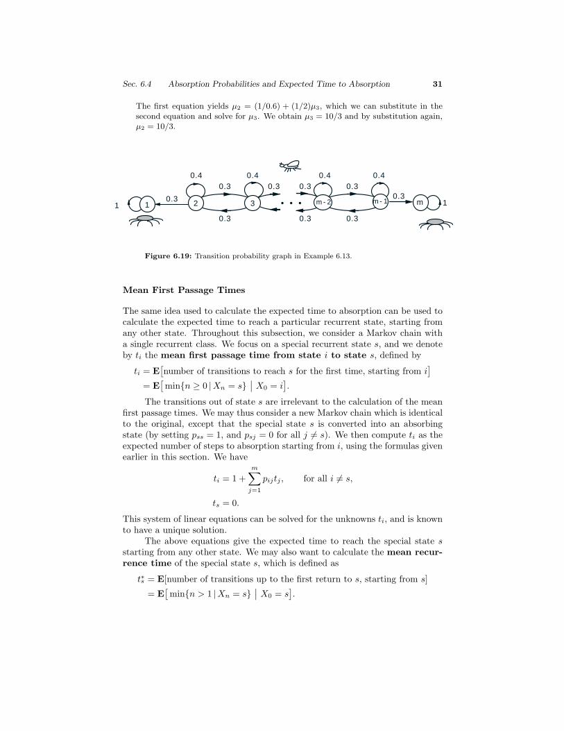
Example 6.13. (Spiders and Fly) Consider the spiders-and-fly model of Ex-ample 6.2. This corresponds to the Markov chain shown in Fig. 6.19. The statescorrespond to possible fly positions, and the absorbing states 1 and m correspondto capture by a spider.
Let us calculate the expected number of steps until the fly is captured. Wehave
µ1 = µm = 0,
and
µi = 1 + 0.3 · µi−1 + 0.4 · µi + 0.3 · µi+1, for i = 2, . . . , m − 1.
We can solve these equations in a variety of ways, such as for example bysuccessive substitution. As an illustration, let m = 4, in which case, the equationsreduce to
µ2 = 1 + 0.4 · µ2 + 0.3 · µ3, µ3 = 1 + 0.3 · µ2 + 0.4 · µ3.
Sec. 6.4 Absorption Probabilities and Expected Time to Absorption 31
The first equation yields µ2 = (1/0.6) + (1/2)µ3, which we can substitute in thesecond equation and solve for µ3. We obtain µ3 = 10/3 and by substitution again,µ2 = 10/3.
2 . . . m - 21
0.4 0.4 0.4 0.4
m - 1
0.3 0.3 0.3 0.3
0.3 0.3 0.3
0.31 3 m 1
0.3
Figure 6.19: Transition probability graph in Example 6.13.
Mean First Passage Times
The same idea used to calculate the expected time to absorption can be used tocalculate the expected time to reach a particular recurrent state, starting fromany other state. Throughout this subsection, we consider a Markov chain witha single recurrent class. We focus on a special recurrent state s, and we denoteby ti the mean first passage time from state i to state s, defined by
ti = E[number of transitions to reach s for the first time, starting from i
]= E
[min{n ≥ 0 |Xn = s}
∣∣ X0 = i].
The transitions out of state s are irrelevant to the calculation of the meanfirst passage times. We may thus consider a new Markov chain which is identicalto the original, except that the special state s is converted into an absorbingstate (by setting pss = 1, and psj = 0 for all j �= s). We then compute ti as theexpected number of steps to absorption starting from i, using the formulas givenearlier in this section. We have
ti = 1 +m∑
j=1
pijtj , for all i �= s,
ts = 0.
This system of linear equations can be solved for the unknowns ti, and is knownto have a unique solution.
The above equations give the expected time to reach the special state sstarting from any other state. We may also want to calculate the mean recur-rence time of the special state s, which is defined as
t∗s = E[number of transitions up to the first return to s, starting from s]
= E[min{n > 1 |Xn = s}
∣∣ X0 = s].
32 Markov Chains Chap. 6
We can obtain t∗s, once we have the first passage times ti, by using the equation
t∗s = 1 +m∑
j=1
psjtj .
To justify this equation, we argue that the time to return to s, starting from s,is equal to 1 plus the expected time to reach s from the next state, which is jwith probability psj . We then apply the total expectation theorem.
Example 6.14. Consider the “up-to-date”–“behind” model of Example 6.1.States 1 and 2 correspond to being up-to-date and being behind, respectively, andthe transition probabilities are
p11 = 0.8, p12 = 0.2,
p21 = 0.6, p22 = 0.4.
Let us focus on state s = 1 and calculate the mean first passage time to state 1,starting from state 2. We have t1 = 0 and
t2 = 1 + p21t1 + p22t2 = 1 + 0.4 · t2,from which
t2 =1
0.6=
5
3.
The mean recurrence time to state 1 is given by
t∗1 = 1 + p11t1 + p12t2 = 1 + 0 + 0.2 · 5
3=
4
3.
Summary of Facts About Mean First Passage Times
Consider a Markov chain with a single recurrent class, and let s be a par-ticular recurrent state.
• The mean first passage times ti to reach state s starting from i, arethe unique solution to the system of equations
ts = 0, ti = 1 +m∑
j=1
pijtj , for all i �= s.
• The mean recurrence time t∗s of state s is given by
t∗s = 1 +m∑
j=1
psjtj .

Sec. 6.5 More General Markov Chains 33
6.5 MORE GENERAL MARKOV CHAINS
The discrete-time, finite-state Markov chain model that we have considered sofar is the simplest example of an important Markov process. In this section,we briefly discuss some generalizations that involve either a countably infinitenumber of states or a continuous time, or both. A detailed theoretical develop-ment for these types of models is beyond our scope, so we just discuss their mainunderlying ideas, relying primarily on examples.
Chains with Countably Infinite Number of States
Consider a Markov process {X1, X2, . . .} whose state can take any positive inte-ger value. The transition probabilities
pij = P(Xn+1 = j |Xn = i), i, j = 1, 2, . . .
are given, and can be used to represent the process with a transition probabilitygraph that has an infinite number of nodes, corresponding to the integers 1, 2, . . .
It is straightforward to verify, using the total probability theorem in asimilar way as in Section 6.1, that the n-step transition probabilities
rij(n) = P(Xn = j |X0 = i), i, j = 1, 2, . . .
satisfy the Chapman-Kolmogorov equations
rij(n + 1) =∞∑
k=1
rik(n)pkj , i, j = 1, 2, . . .
Furthermore, if the rij(n) converge to steady-state values πj as n → ∞, then bytaking limit in the preceding equation, we obtain
πj =∞∑
k=1
πkpkj , i, j = 1, 2, . . .
These are the balance equations for a Markov chain with states 1, 2, . . .It is important to have conditions guaranteeing that the rij(n) indeed con-
verge to steady-state values πj as n → ∞. As we can expect from the finite-statecase, such conditions should include some analog of the requirement that thereis a single recurrent class that is aperiodic. Indeed, we require that:
(a) each state is accessible from every other state;
(b) the set of all states is aperiodic in the sense that there is no d > 1 suchthat the states can be grouped in d > 1 disjoint subsets S1, . . . , Sd so thatall transitions from one subset lead to the next subset.
34 Markov Chains Chap. 6
These conditions are sufficient to guarantee the convergence to a steady-state
limn→∞
rij(n) = πj , i, j = 1, 2, . . .
but something peculiar may also happen here, which is not possible if the numberof states is finite: the limits πj may not add to 1, so that (π1, π2, . . .) may notbe a probability distribution. In fact, we can prove the following theorem (theproof is beyond our scope).
Steady-State Convergence Theorem
Under the above accessibility and aperiodicity assumptions (a) and (b),there are only two possibilities:
(1) The rij(n) converge to a steady state probability distribution (π1, π2, . . .).In this case the πj uniquely solve the balance equations together withthe normalization equation π1 + π2 + · · · = 1. Furthermore, the πj
have an expected frequency interpretation:
πj = limn→∞
vij(n)n
,
where vij(n) is the expected number of visits to state j within the firstn transitions, starting from state i.
(2) All the rij(n) converge to 0 as n → ∞ and the balance equations haveno solution, other than πj = 0 for all j.
For an example of possibility (2) above, consider the packet queueing sys-tem of Example 6.10 for the case where the probability b of a packet arrival ineach period is larger than the probability d of a departure. Then, as we sawin that example, as the buffer size m increases, the size of the queue will tendto increase without bound, and the steady-state probability of any one statewill tend to 0 as m → ∞. In effect, with infinite buffer space, the system is“unstable” when b > d, and all states are “transient.”
An important consequence of the steady-state convergence theorem is thatif we can find a probability distribution (π1, π2, . . .) that solves the balance equa-tions, then we can be sure that it is the steady-state distribution. This line ofargument is very useful in queueing systems as illustrated in the following twoexamples.
Example 6.15. (Queueing with Infinite Buffer Space) Consider, as in Ex-ample 6.10, a communication node, where packets arrive and are stored in a bufferbefore getting transmitted. We assume that the node can store an infinite number

Sec. 6.5 More General Markov Chains 35
of packets. We discretize time in very small periods, and we assume that in eachperiod, one of the following occurs:
(a) one new packet arrives; this happens with a given probability b > 0;
(b) one existing packet completes transmission; this happens with a given prob-ability d > 0 if there is at least one packet in the node, and with probability0 otherwise;
(c) no new packet arrives and no existing packet completes transmission; thishappens with a probability 1−b−d if there is at least one packet in the node,and with probability 1 − b otherwise.
. . . b
d
0 1 . . . m - 1 m
b
d
1 - b - d1 - b
bb b
d d d
1 - b - d 1 - b - d
Figure 6.20: Transition probability graph in Example 6.15.
We introduce a Markov chain with states are 0, 1, . . ., corresponding to thenumber of packets in the buffer. The transition probability graph is given inFig. 6.20. As in the case of a finite number of states, the local balance equationsare
πib = πi+1d, i = 0, 1, . . . ,
and we obtain πi+1 = ρπi, where ρ = b/d. Thus, we have πi = ρiπ0 for all i. Ifρ < 1, the normalization equation 1 =
∑∞i=0
πi yields
1 = π0
∞∑i=0
ρi =π0
1 − ρ,
in which case π0 = 1 − ρ, and the steady-state probabilities are
πi = ρi(1 − ρ), i = 0, 1, . . .
If ρ ≥ 1, which corresponds to the case where the arrival probability b is no lessthan the departure probability d, the normalization equation 1 = π0(1+ρ+ρ2+· · ·)implies that π0 = 0, and also πi = ρiπ0 = 0 for all i.
Example 6.16. (The M/G/1 Queue) Packets arrive at a node of a communi-cation network, where they are stored at an infinite capacity buffer and are thentransmitted one at a time. The arrival process of the packets is Poissson with rate

36 Markov Chains Chap. 6
λ, and the transmission time of a packet has a given CDF. Furthermore, the trans-mission times of different packets are independent and are also independent fromall the interarrival times of the arrival process.
This queueing system is known as the M/G/1 system. With changes in ter-minology, it applies to many different practical contexts where “service” is providedto “arriving customers,” such as in communication, transportation, and manufac-turing, among others. The name M/G/1 is an example of shorthand terminologyfrom queueing theory, whereby the first letter (M in this case) characterizes thecustomer arrival process (Poisson in this case), the second letter (G in this case)characterizes the distribution of the service time of the queue (general in this case),and the number (1 in this case) characterizes the number of customers that can besimultaneously served.
To model this system as a discrete-time Markov chain, we focus on the timeinstants when a packet completes transmission and departs from the system. Wedenote by Xn the number of packets in the system just after the nth customer’sdeparture. We have
Xn+1 ={
Xn − 1 + Sn if Xn > 0,Sn if Xn = 0,
where Sn is the number of packet arrivals during the (n+1)st packet’s transmission.In view of the Poisson assumption, the random variables S1, S2, . . . are independentand their PMF can be calculated using the given CDF of the transmission time,and the fact that in an interval of length r, the number of packet arrivals is Poisson-distributed with parameter λr. In particular, let us denote
αk = P(Sn = k), k = 0, 1, . . . ,
and let us assume that if the transmission time R of a packet is a discrete randomvariable taking the values r1, . . . , rm with probabilities p1, . . . , pm. Then, we havefor all k ≥ 0,
αk =
m∑j=1
pje−λrj (λrj)
k
k!,
while if R is a continuous random variable with PDF fR(r), we have for all k ≥ 0,
αk =
∫ ∞
r=0
P(Sn = k |R = r)fR(r) dr =
∫ ∞
r=0
e−λr(λr)k
k!fR(r) dr.
The probabilities αk define in turn the transition probabilities of the Markov chain{Xn}, as follows (see Fig. 6.21):
pij =
{αj if i = 0 and j > 0,αj−i+1 if i > 0 and j ≥ i − 1,0 otherwise.
Clearly, this Markov chain satisfies the accessibility and aperiodicity condi-tions that guarantee steady-state convergence. There are two possibilities: either(π0, π1, . . .) form a probability distribution, or else πj > 0 for all j. We will clarify

Sec. 6.5 More General Markov Chains 37
0 1 . . .
α0
2 3
α0
α1
α1 α1
α0 α0
α1α2 α2
α2
α3
α3
Figure 6.21: Transition probability graph for the number of packets leftbehind by a packet completing transmission in the M/G/1 queue (Example6.16).
the conditions under which each of these cases holds, and we will also calculate thetransform M(s) (when it exists) of the steady-state distribution (π0, π1, . . .):
M(s) =
∞∑j=0
πjesj .
For this purpose, we will use the transform of the PMF {αk}:
A(s) =
∞∑j=0
αjesj .
Indeed, let us multiply the balance equations
πj = π0αj +
j+1∑i=1
πiαj−i+1,
with esj and add over all j. We obtain
M(s) =
∞∑j=0
π0αjesj +
∞∑j=0
(j+1∑i=1
πiαj−i+1
)esj
= A(s) +
∞∑i=1
πies(i−1)
∞∑j=i−1
αj−i+1es(j−i+1)
= A(s) +A(s)
es
∞∑i=1
πiesi
= A(s) +A(s)
(M(s) − π0
)es
,
or
M(s) =(es − 1)π0A(s)
es − A(s).

38 Markov Chains Chap. 6
To calculate π0, we take the limit as s → 0 in the above formula, and we use thefact M(0) = 1 when {πj} is a probability distribution. We obtain, using the factA(0) = 1 and L’Hospital’s rule,
1 = lims→0
(es − 1)π0A(s)
es − A(s)=
π0
1−(dA(s)/ds
)∣∣s=0
=π0
1 − E[N ],
where E[N ] =∑∞
j=0jαj is the expected value of the number N of packet arrivals
within a packet’s transmission time. Using the iterated expectations formula, wehave
E[N ] = λE[R],
where E[R] is the expected value of the transmission time. Thus,
π0 = 1 − λE[R],
and the transform of the steady-state distribution {πj} is
M(s) =(es − 1)
(1 − λE[R]
)A(s)
es − A(s).
For the above calculation to be correct, we must have E[N ] < 1, i.e., packets shouldarrive at a rate that is smaller than the transmission rate of the node. If this is nottrue, the system is not “stable” and there is no steady-state distribution, i.e., theonly solution of the balance equations is πj = 0 for all j.
Let us finally note that we have introduced the πj as the steady-state prob-ability that j packets are left behind in the system by a packet upon completingtransmission. However, it turns out that πj is also equal to the steady-state prob-ability of j packets found in the system by an observer that looks at the system ata “typical” time far into the future. This is discussed in the theoretical problems,but to get an idea of the underlying reason, note that for each time the number ofpackets in the system increases from n to n + 1 due to an arrival, there will be acorresponding future decrease from n + 1 to n due to a departure. Therefore, inthe long run, the frequency of transitions from n to n + 1 is equal to the frequencyof transitions from n + 1 to n. Therefore, in steady-state, the system appearsstatistically identical to an arriving and to a departing packet. Now, because thepacket interarrival times are independent and exponentially distributed, the timesof packet arrivals are “typical” and do not depend on the number of packets inthe system. With some care this argument can be made precise, and shows thatat the times when packets complete their transmissions and depart, the system is“typically loaded.”
Continuous-Time Markov Chains
We have implicitly assumed so far that the transitions between states take unittime. When the time between transitions takes values from a continuous range,some new questions arise. For example, what is the proportion of time that the
Sec. 6.5 More General Markov Chains 39
system spends at a particular state (as opposed to the frequency of visits intothe state)?
Let the states be denoted by 1, 2, . . ., and let us assume that state tran-sitions occur at discrete times, but the time from one transition to the next israndom. In particular, we assume that:
(a) If the current state is i, the next state will be j with a given probabilitypij .
(b) The time interval ∆i between the transition to state i and the transitionto the next state is exponentially distributed with a given parameter νi:
P(∆i ≤ δ | current state is i) ≤ 1 − e−νiδ.
Furthermore, ∆i is independent of earlier transition times and states.
The parameter νi is referred to as the transition rate associated with statei. Since the expected transition time is
E[∆i] =∫ ∞
0
δνie−νiδdδ =1νi
,
we can interpret νi as the average number of transitions per unit time. We mayalso view
qij = pijνi
as the rate at which the process makes a transition to j when at state i. Con-sequently, we call qij the transition rate from i to j. Note that given thetransition rates qij , one can obtain the node transition rates using the formulaνi =
∑∞j=1 qij .
The state of the chain at time t ≥ 0 is denoted by X(t), and stays constantbetween transitions. Let us recall the memoryless property of the exponentialdistribution, which in our context implies that, for any time t between the kthand (k + 1)st transition times tk and tk+1, the additional time tk+1 − t neededto effect the next transition is independent of the time t − tk that the systemhas been in the current state. This implies the Markov character of the process,i.e., that at any time t, the future of the process, [the random variables X(t) fort > t] depend on the past of the process [the values of the random variables X(t)for t ≤ t] only through the present value of X(t).
Example 6.17. (The M/M/1 Queue) Packets arrive at a node of a communi-cation network according to a Poissson process with rate λ. The packets are storedat an infinite capacity buffer and are then transmitted one at a time. The trans-mission time of a packet is exponentially distributed with parameter µ, and thetransmission times of different packets are independent and are also independentfrom all the interarrival times of the arrival process. Thus, this queueing system isidentical to the special case of the M/G/1 system, where the transmission times areexponentially distributed (this is indicated by the second M inthe M/M/1 name).

40 Markov Chains Chap. 6
We will model this system using a continuous-time process with state X(t)equal to the number of packets in the system at time t [if X(t) > 0, then X(t) − 1packets are waiting in the queue and one packet is under transmission]. The stateincreases by one when a new packet arrives and decreases by one when an existingpacket departs. To show that this process is a continuous-time Markov chain, letus identify the transition rates νi and qij at each state i.
Consider first the case where at some time t, the system becomes empty,i.e., the state becomes equal to 0. Then the next transition will occur at the nextarrival, which will happen in time that is exponentially distributed with parameterλ. Thus at state 0, we have the transition rates
q0j ={
λ if j = 1,0 otherwise.
Consider next the case of a positive state i, and suppose that a transition oc-curs at some time t to X(t) = i. If the next transition occurs at time t+∆i, then ∆i
is the minimum of two exponentially distributed random variables: the time to thenext arrival, call it Y, which has parameter λ, and the time to the next departure,call it Z, which has parameter µ. (We are again using here the memoryless propertyof the exponential distribution.) Thus according to Example 5.15, which deals with“competing exponentials,” the time ∆i is exponentially distributed with parameterνi = λ + µ. Furthermore, the probability that the next transition corresponds toan arrival is
P(Y ≤ Z) =
∫y≤z
λe−λy · µeµz dy dz
= λµ
∫ ∞
0
e−λy
(∫ ∞
y
eµz dz
)dy
= λµ
∫ ∞
0
e−λy
(e−µy
µ
)dy
= λ
∫ ∞
0
e−(λ+µ)y dy
=λ
λ + µ.
We thus have for i > 0, qi,i+1 = νiP(Y ≤ Z) = (λ + µ)(λ/(λ + µ)
)= λ. Similarly,
we obtain that the probability that the next transition corresponds to a departureis µ/(λ + µ), and we have qi,i−1 = νiP(Y ≥ Z) = (λ + µ)
(µ/(λ + µ)
)= µ. Thus
qij =
{λ if j = i + 1,µ if j = i − 1,0 otherwise.
The positive transition rates qij are recorded next to the arcs (i, j) of the transitiondiagram, as in Fig. 6.22.
We will be interested in chains for which the discrete-time Markov chaincorresponding to the transition probabilities pij satisfies the accessibility and

Sec. 6.5 More General Markov Chains 41
. . . 0 1 . . . m - 1 m
λ
µ
λ λ λ λ
µ µ µµ
Figure 6.22: Transition graph for the M/M/1 queue (Example 6.17).
aperiodicity assumptions of the preceding section. We also require a technicalcondition, namely that the number of transitions in any finite length of timeis finite with probability one. Almost all models of practical use satisfy thiscondition, although it is possible to construct examples that do not.
Under the preceding conditions, it can be shown that the limit
πj = limt→∞
P(X(t) = j |X(0) = i
)exists and is independent of the initial state i. We refer to πj as the steady-stateprobability of state j. It can be shown that if Tj(t) is the expected value of thetime spent in state j up to time t, then, regardless of the initial state, we have
πj = limt→∞
Tj(t)t
that is, πj can be viewed as the long-term proportion of time the process spendsin state j.
The balance equations for a continuous-time Markov chain take the form
pj
∞∑i=0
qji =∞∑
i=0
piqij , j = 0, 1, . . .
Similar to discrete-time Markov chains, it can be shown that there are twopossibilities:
(1) The steady-state probabilities are all positive and solve uniquely the bal-ance equations together with the normalization equation π1 +π2 + · · · = 1.
(2) The steady-state probabilities are all zero.
To interpret the balance equations, we note that since πi is the proportionof time the process spends in state i, it follows that πiqij can be viewed asfrequency of transitions from i to j (expected number of transitions from i toj per unit time). It is seen therefore that the balance equations express theintuitive fact that the frequency of transitions out of state j (the left side termπj
∑∞i=1 qji) is equal to the frequency of transitions into state j (the right side
term∑∞
i=0 πiqij).The continuous-time analog of the local balance equations for discrete-time
chains isπjqji = πiqij , i, j = 1, 2, . . .
42 Markov Chains Chap. 6
These equations hold in birth-death systems where qij = 0 for |i − j| > 1, butneed not hold in other types of Markov chains. They express the fact that thefrequencies of transitions from i to j and from j to i are equal.
To understand the relationship between the balance equations for continuous-time chains and the balance equations for discrete-time chains, consider anyδ > 0, and the discrete-time Markov chain {Zn |n ≥ 0}, where
Zn = X(nδ), n = 0, 1, . . .
The steady-state distribution of {Zn} is clearly {πj | j ≥ 0}, the steady-statedistribution of the continuous chain. The transition probabilities of {Zn |n ≥ 0}can be derived by using the properties of the exponential distribution. We obtain
pij = δqij + o(δ), i �= j,
pjj = 1 − δ
∞∑i=0i �=j
qji + o(δ)
Using these expressions, the balance equations
πj =∞∑
i=0
πi pij j ≥ 0
for the discrete-time chain {Zn}, we obtain
πj =∞∑
i=0
πipij = pj
(1 − δ
∞∑i=0i �=j
qji + o(δ))
+∑i=0i �=j
pi
(δqij + o(δ)
).
Taking the limit as δ → 0, we obtain the balance equations for the continuous-time chain.
Example 6.18. (The M/M/1 Queue – Continued) As in the case of a finitenumber of states, the local balance equations are
πiλ = πi+1µ, i = 0, 1, . . . ,
and we obtain πi+1 = ρπi, where ρ = λ/µ. Thus, we have πi = ρiπ0 for all i. Ifρ < 1, the normalization equation 1 =
∑∞i=0
πi yields
1 = π0
∞∑i=0
ρi =π0
1 − ρ,
in which case π0 = 1 − ρ, and the steady-state probabilities are
πi = ρi(1 − ρ), i = 0, 1, . . .

Sec. 6.5 More General Markov Chains 43
If ρ ≥ 1, which corresponds to the case where the arrival probability b is no lessthan the departure probability d, the normalization equation 1 = π0(1+ρ+ρ2+· · ·)implies that π0 = 0, and also πi = ρiπ0 = 0 for all i.
Example 6.19. (The M/M/m and M/M/∞ Queues) The M/M/m queueingsystem is identical to the M/M/1 system except that m packets can be simul-taneously transmitted (i.e., the transmission line of the node has m transmissionchannels). A packet at the head of the queue is routed to any channel that isavailable. The corresponding state transition diagram is shown in Fig. 6.24.
. . . λ
mµ
0 1 . . . m - 1 m
λ
µ
λ λ λ
2µ (m - 1)µ mµmµ
m+1
λ
Figure 6.24: Transition graph for the M/M/m queue (Example 6.19).
By writing down the local balance equations for the steady-state probabilitiesπn, we obtain
λπn−1 ={
nµπn if n ≤ m,mµπn if n > m.
From these equations, we obtain
πn =
p0(mρ)n
n!, n ≤ m
p0mmρn
m!, n > m
where ρ is given by
ρ =λ
mµ.
Assuming ρ < 1, we can calculate π0 using the above equations and the condition∑∞n=0
πn = 1. We obtain
π0 =
(1 +
m−1∑n=1
(mρ)n
n!+
∞∑n=m
(mρ)n
m!
1
mn−m
)−1
and, finally,
π0 =
(m−1∑n=0
(mρ)n
n!+
(mρ)m
m!(1 − ρ)
)−1
.

44 Markov Chains Chap. 6
In the limiting case where m = ∞ in the M/M/m system (which is calledthe M/M/∞ system), the local balance equations become
λπn−1 = nµπn, n = 1, 2, . . .
so
πn = π0
(λ
µ
)n1
n!, n = 1, 2, . . .
From the condition∑∞
n=0πn = 1, we obtain
π0 =
(1 +
∞∑n=1
(λ
µ
)n1
n!
)−1
= e−λ/µ,
so, finally,
πn =
(λ
µ
)ne−λ/µ
n!, n = 0, 1, . . .
Therefore, in steady-state, the number in the system is Poisson distributed withparameter λ/µ.