6. introduction and chapter objectives - digilentinc · ©2012 digilent,inc. 1 6. introduction and...

Real Analog - Circuits 1Chapter 6: Energy Storage Elements

© 2012 Digilent, Inc. 1

6. Introduction and Chapter ObjectivesSo far, we have considered circuits that have been governed by algebraic relations. These circuits have, in general,contained only power sources and resistive elements. All elements in these circuits, therefore, have either suppliedpower from external sources or dissipated power. For these resistive circuits, we can apply either time-varying orconstant signals to the circuit without really affecting our analysis approach. Ohm’s law, for example, is equallyapplicable to time-varying or constant voltages and currents:

RtitvRIV )()(

Since the governing equation is algebraic, it is applicable at every point in time – voltages and currents at a pointin time are affected only by voltages and currents at the same point in time.

We will now begin to consider circuit elements, which are governed by differential equations. These circuitelements are called dynamic circuit elements or energy storage elements. Physically, these circuit elements storeenergy, which they can later release back to the circuit. The response, at a given time, of circuits that contain theseelements is not only related to other circuit parameters at the same time; it may also depend upon the parametersat other times.

This chapter begins with an overview of the basic concepts associated with energy storage. This discussion focusesnot on electrical systems, but instead introduces the topic qualitatively in the context of systems with which thereader is already familiar. The goal is to provide a basis for the mathematics, which will be introducedsubsequently. Since we will now be concerned with time-varying signals, section 6.2 introduces the basic signalsthat we will be dealing with in the immediate future. This chapter concludes with presentations of the twoelectrical energy storage elements that we will be concerned with: capacitors and inductors. The method by whichenergy is stored in these elements is presented in sections 6.3 and 6.4, along with the governing equations relatingvoltage and current for these elements.

Real Analog – Circuits 1Chapter 6: Energy Storage Elements


After completing this chapter, you should be able to:

Qualitatively state the effect of energy storage on the type of mathematics governing a system Define transient response Define steady-state response Write the mathematical expression for a unit step function Sketch the unit step function Sketch shifted and scaled versions of the unit step function Write the mathematical expression for a decaying exponential function Define the time constant of an exponential function Sketch a decaying exponential function, given the function’s initial value and time constant Use a unit step function to restrict an exponential function to times greater than zero Write the circuit symbol for a capacitor State the mechanism by which a capacitor stores energy State the voltage-current relationship for a capacitor in both differential and integral form State the response of a capacitor to constant voltages and instantaneous voltage changes Write the mathematical expression describing energy storage in a capacitor Determine the equivalent capacitance of series and parallel combinations of capacitors Sketch a circuit describing a non-ideal capacitor Write the circuit symbol for an inductor State the mechanism by which an inductor stores energy State the voltage-current relationship for an inductor in both differential and integral form State the response of an inductor to constant voltages and instantaneous current changes Write the mathematical expression describing energy storage in an inductor Determine the equivalent inductance of series and parallel combinations of inductors Sketch a circuit describing a non-ideal inductor

Real Analog – Circuits 1Chapter 6.1: Fundamental Concepts


6.1: Fundamental ConceptsThis section provides a brief overview of what it meant by energy storage in terms of a system-level description ofsome physical process. Several examples of energy storage elements are presented, for which the reader shouldhave an intuitive understanding. These examples are intended to introduce the basic concepts in a qualitativemanner; the mathematical analysis of dynamic systems will be provided in later chapters.

We have previously introduced the concept of representing a physical process as a system. In this viewpoint, thephysical process has an input and an output. The input to the system is generated from sources external to thesystem – we will consider the input to the system to be a known function of time. The output of the system is thesystem’s response to the input. The input-output equation governing the system provides the relationshipbetween the system’s input and output. A general input-output equation has the form:

(6.1)

The process is shown in block diagram form in Figure 6.1.

Figure 6.1. Block diagram representation of a system.

The system of Figure 6.1 transfers the energy in the system input to the system output. This process transformsthe input signal u(t) into the output signal y(t). In order to perform this energy transfer, the system will, ingeneral, contain elements that both store and dissipate energy. To date, we have analyzed systems which containonly energy dissipation elements. We review these systems briefly below in a systems context. Subsequently, weintroduce systems that store energy; our discussion of energy storage elements is mainly qualitative in this chapterand presents systems for which the reader should have an intuitive understanding.

Systems with no energy storage:

In previous chapters, we considered cases in which the input-output equation is algebraic. This implies that theprocesses being performed by the system involve only sources and components which dissipate energy. Forexample, output voltage of the inverting voltage amplifier of Figure 6.2 is:

inin

fOUT V

RR

V

(6.2)

This circuit contains only resistors (in the form of Rf and Rin) and sources (in the form of Vin and the op-amppower supplies) and the equation relating the input and output is algebraic. Note that the op-amp power suppliesdo not appear in equation (6.2), since linear operation of the circuit of Figure 6.2 implies that the output voltage isindependent of the op-amp power supplies.

)}({)( tufty



Figure 6.2. Inverting voltage amplifier.

One side effect of an algebraic input-output equation is that the output responds instantaneously to any changesin the input. For example, consider the circuit shown in Figure 6.3. The input voltage is based on the position ofa switch; when the switch closes, the input voltage applied to the circuit increases instantaneously from 0V to 2V.Figure 6.3 indicates that the switch closes at time t = 5 seconds; thus, the input voltage as a function of time is asshown in Figure 6.4(a). For the values of Rf and Rin shown in Figure 6.3, the input-output equation becomes:

)(5)( tVtV inOUT (6.3)

and the output voltage as a function of time is as shown in Figure 6.4(b). The output voltage respondsimmediately to the change in the input voltage.

Figure 6.3. Switched voltage amplifier.

(a) Input voltage (b) Output voltage

Figure 6.4. Input and output signals for circuit of Figure 3.



Systems with energy storage:

We now consider systems, which contain energy storage elements. The inclusion of energy storage elementsresults in the input-output equation for the system, which is a differential equation. We present the concepts interms of two examples for which the reader most likely has some expectations based on experience and intuition.

Example 6.1: Mass-damper system

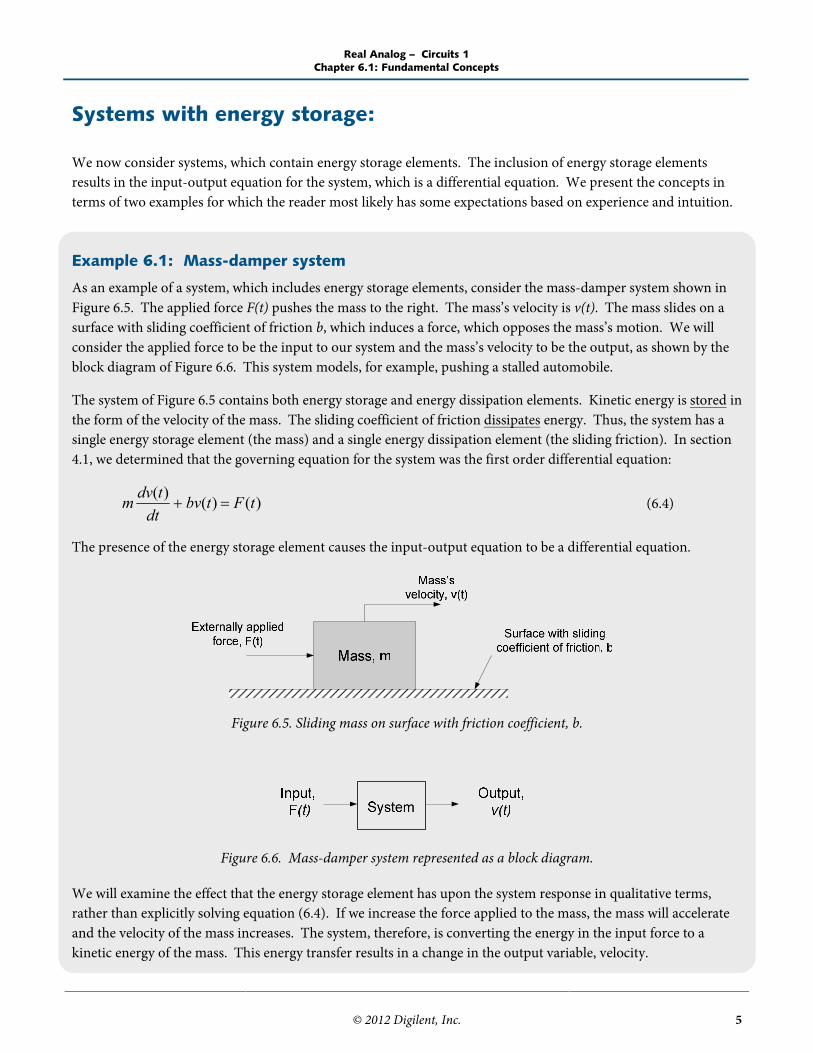
As an example of a system, which includes energy storage elements, consider the mass-damper system shown inFigure 6.5. The applied force F(t) pushes the mass to the right. The mass’s velocity is v(t). The mass slides on asurface with sliding coefficient of friction b, which induces a force, which opposes the mass’s motion. We willconsider the applied force to be the input to our system and the mass’s velocity to be the output, as shown by theblock diagram of Figure 6.6. This system models, for example, pushing a stalled automobile.

The system of Figure 6.5 contains both energy storage and energy dissipation elements. Kinetic energy is stored inthe form of the velocity of the mass. The sliding coefficient of friction dissipates energy. Thus, the system has asingle energy storage element (the mass) and a single energy dissipation element (the sliding friction). In section4.1, we determined that the governing equation for the system was the first order differential equation:

)()()( tFtbvdttdvm (6.4)

The presence of the energy storage element causes the input-output equation to be a differential equation.

Figure 6.5. Sliding mass on surface with friction coefficient, b.

Figure 6.6. Mass-damper system represented as a block diagram.

We will examine the effect that the energy storage element has upon the system response in qualitative terms,rather than explicitly solving equation (6.4). If we increase the force applied to the mass, the mass will accelerateand the velocity of the mass increases. The system, therefore, is converting the energy in the input force to akinetic energy of the mass. This energy transfer results in a change in the output variable, velocity.



The energy storage elements of the system of Figure 6.5 do not, however, allow an instantaneous change invelocity to an instantaneous change in force. For example, say that before time t = 0 no force is applied to themass and the mass is at rest. At time t = 0 we suddenly apply a force to the mass, as shown in Figure 6.7(a) below.At time t = 0 the mass begins to accelerate but it takes time for the mass to approach its final velocity, as shown inFigure 6.7(b). This transitory stage, when the system is in transition from one constant operating condition toanother is called the transient response. After a time, the energy input from the external force is balanced by theenergy dissipated by the sliding friction, and the velocity of the mass remains constant. When the operatingconditions are constant, the energy input is exactly balanced by the energy dissipation, and the system’s responseis said to be in steady-state. We will discuss these terms in more depth in later chapters when we perform themathematical analysis of dynamic systems.

Figure 6.7(a). Force applied to mass.

Figure 6.7(b). Velocity of mass.



Example 6.2: Heating a mass

Our second example of a system, which includes energy storage elements, is a body that is subjected to some heatinput. The overall system is shown in Figure 6.8. The body being heated has some mass m, specific heat cP, andtemperature TB. Some heat input qin is applied to the body from an external source, and the body transfers heatqout to its surroundings. The surroundings are at some ambient temperature T0. We will consider the input to oursystem to be the applied heat input qin and the output to be the temperature of the body TB, as shown in the blockdiagram of Figure 6.9. This system is a model, for example, of the process of heating a frying pan on a stove. Heatinput is applied by the stove burner and the pan dissipates heat by transferring it to the surroundings.

Figure 6.8. Body subjected to heating.

Figure 6.9. System block diagram.

The system of Figure 6.8 contains both energy storage and energy dissipation elements. Energy is stored in theform of the temperature of the mass. Energy is dissipated in the form of heat transferred to the surroundings.Thus, the system has a single energy storage element (the mass) and a single energy dissipation element (the heatdissipation). The governing equation for the system is the first order differential equation:

inOUTB

P qqdtTTd

mc )( 0 (6.5)

The presence of the energy storage element causes the input-output equation to be a differential equation.

We again examine the response of this system to some input in qualitative rather than quantitative terms in orderto provide some insight into the overall process before immersing ourselves in the mathematics associated withanalyzing the system quantitatively. If the heat input to the system is increased instantaneously (for example, if we



suddenly turn up the heat setting on our stove burner) the mass’s temperature will increase. As the mass’stemperature increases, the heat transferred to the ambient surroundings will increase. When the heat input to themass is exactly balanced by the heat transfer to the surroundings, the mass’s temperature will no longer changeand the system will be at a steady-state operating condition. Since the mass provides energy storage, thetemperature of the mass will not respond instantaneously to a sudden change in heat input – the temperature willrise relatively slowly to its steady-state operating condition. (We know from experience that changing the burnersetting on the stove does not immediately change the temperature of our pan, particularly if the pan is heavy.)The process of changing the body’s temperature from one steady state operating condition to another is thesystem’s transient response.

The process of changing the body’s temperature by instantaneously increasing the heat input to the body isillustrated in Figure 6.10. The signal corresponding to the heat input is shown in Figure 6.10(a), while theresulting temperature response of the body is shown in Figure 6.10(b).

(a) Heat input (b) Temperature response

Figure 6.10. Temperature response to instantaneous heat input.



Section Summary:

Systems with energy storage elements are governed by differential equations. Systems that contain onlyenergy dissipation elements (such as resistors) are governed by algebraic equations.

The responses of systems governed by algebraic equations will typically have the same “shape” as the input.The output at a given time is simply dependent upon the input at that same time – the system does not“remember” any previous conditions.

The responses of systems governed by differential equations will not, in general, have the same “shape” as theforcing function applied to the system. The system “remembers” previous conditions – this is why thesolution to a differential equation requires knowledge of initial conditions.

The response of a system that stores energy is generally considered to consist of two parts: the transientresponse and the steady-state response. These are described as follows:1. The transient response typically is shaped differently from the forcing function. It is due to initial energy

levels stored in the system.2. The steady-state response is the response of the system as t→∞. It is the same “shape” as the forcing

function applied to the system.In differential equations courses, the transient response corresponds (approximately) to the homogeneoussolution of the governing differential equation, while the steady-state response corresponds to the particularsolution of the governing differential equation.

Exercises:

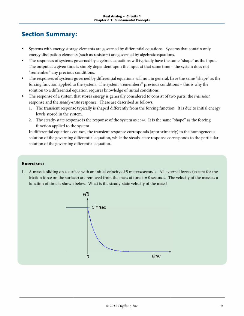
1. A mass is sliding on a surface with an initial velocity of 5 meters/seconds. All external forces (except for thefriction force on the surface) are removed from the mass at time t = 0 seconds. The velocity of the mass as afunction of time is shown below. What is the steady-state velocity of the mass?

Real Analog – Circuits 1Chapter 6.2: Basic Time-varying Signals


6.2: Basic Time-varying SignalsSince the analysis of dynamic systems relies upon time-varying phenomenon, this chapter section presents somecommon time-varying signals that will be used in our analyses. Specific signals that will be presented are stepfunctions and exponential functions.

Step Function:

We will use a step function to model a signal, which changes suddenly from one constant value to another. Thesetypes of signals can be very important. Examples include digital logic circuits (which switch between low and highvoltage levels) and control systems (whose design specifications are often based on the system’s response to asudden change in input).

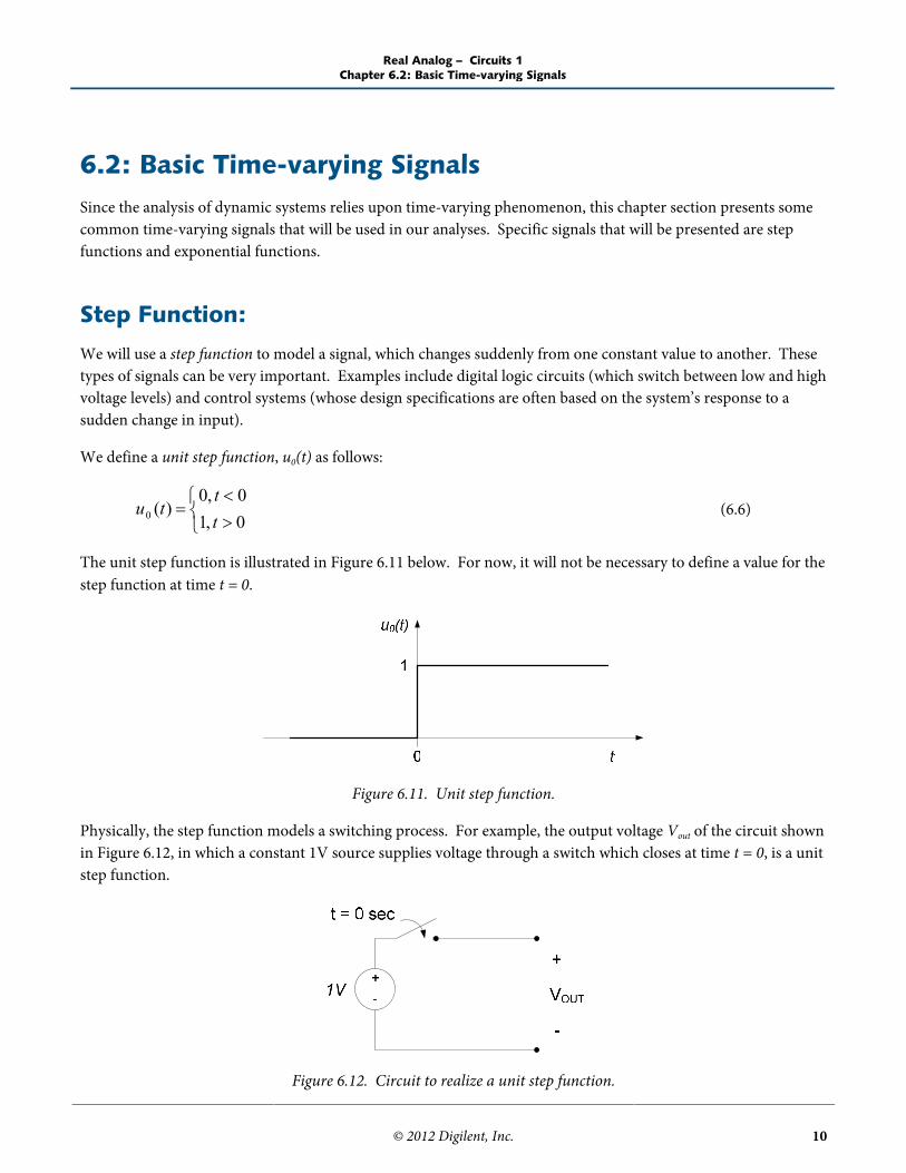
We define a unit step function, u0(t) as follows:

0,10,0

)(0 tt

tu (6.6)

The unit step function is illustrated in Figure 6.11 below. For now, it will not be necessary to define a value for thestep function at time t = 0.

Figure 6.11. Unit step function.

Physically, the step function models a switching process. For example, the output voltage Vout of the circuit shownin Figure 6.12, in which a constant 1V source supplies voltage through a switch which closes at time t = 0, is a unitstep function.

Figure 6.12. Circuit to realize a unit step function.



The unit step function can be scaled to provide different amplitudes. Multiplication of the unit step function by aconstant K results in a signal which is zero for times less than zero and K for times greater than zero, as shown inFigure 6.13.

Figure 6.13. Scaled step function Ku0(t); K>0.

The step function can also be shifted to model processes which switch at times other than t = 0. A step functionwith amplitude K which occurs at time t = a can be written as Ku0(t-a):

atKat

atKu,,0

)(0 (6.7)

The function is zero when the argument t-a is less than zero and K when the argument t-a is greater than zero, asshown in Figure 6.14. If a>0, the function is shifted to the right of the origin; if a<0, the function is shifted to thelet of the origin.

Figure 6.14. Shifted and scaled step function Ku0(t-a); K>0 and a>0.

Switching the sign of the above argument in equation (6.7) results in:

atatK

taKuatKu,0,

)()( 00 (6.8)

and the value of the function is K for t<a and zero for t>a, as shown in Figure 6.15. As above, the transition fromK to zero is to the right of the origin if a>0 and to the left of the origin if a<0.

Figure 6.15. The function step function Ku0(a-t); K>0 and a>0.



Step functions can also be used to describe finite-duration signals. For example, the function:

2,020,10,0

)(ttt

tf

illustrated in Figure 6.16, can be written in terms of sums or products of unit step functions as follows:

)2()()( 00 tututf

or

)2()()( 00 tututf

Figure 6.16. Finite-duration signal.

The step function can also be used to create other finite-duration functions. For example, the finite-durationramp function

1,010,0,0

)(tttt

tf

shown in Figure 6.17, can be written as a single function over the entire range -<t< by using unit stepfunctions, as follows:

)]1()([)( 00 tututtf

Figure 6.17. Finite-duration “ramp” signal.



Exponential Functions:

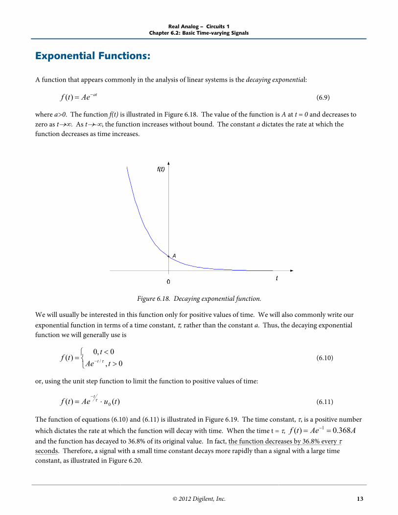
A function that appears commonly in the analysis of linear systems is the decaying exponential:

atAetf )( (6.9)

where a>0. The function f(t) is illustrated in Figure 6.18. The value of the function is A at t = 0 and decreases tozero as t. As t-, the function increases without bound. The constant a dictates the rate at which thefunction decreases as time increases.

Figure 6.18. Decaying exponential function.

We will usually be interested in this function only for positive values of time. We will also commonly write ourexponential function in terms of a time constant, , rather than the constant a. Thus, the decaying exponentialfunction we will generally use is

0,0,0

)( / tAet

tf t (6.10)

or, using the unit step function to limit the function to positive values of time:

)()( 0 tuAetft

(6.11)

The function of equations (6.10) and (6.11) is illustrated in Figure 6.19. The time constant, , is a positive numberwhich dictates the rate at which the function will decay with time. When the time t = , AAetf 368.0)( 1

and the function has decayed to 36.8% of its original value. In fact, the function decreases by 36.8% every seconds. Therefore, a signal with a small time constant decays more rapidly than a signal with a large timeconstant, as illustrated in Figure 6.20.



Figure 6.19. Exponential function )()( 0 tuAetft

.

Figure 6.20. Exponential function variation with time cons



Section Summary:

Step functions are useful for representing conditions (generally inputs), which change from one value toanother instantaneously. In electrical engineering, they are commonly used to model the opening or closingof a switch that connects a circuit to a source, which provides a constant voltage or current. Mathematically,an arbitrary step function can be represented by:

atatK

taKuatKu,0,

)()( 00

So that the step function turns “on” at time t = a, and has an amplitude K.

An exponential function, defined for t>0, is mathematically defined as:

)()( 0 tuAetft

The function has an initial value, A, and a time constant, τ. The time constant indicates how quickly thefunction decays; the value of the function decreases by 63.2% every τ seconds. Exponential functions areimportant to use because the solutions of linear, constant coefficient, ordinary differential equations typicallytake the form of exponentials.



Exercises:

1. Express the signal below in terms of step functions.

2. The function shown below is a decaying exponential. Estimate the function from the given graph.

Real Analog – Circuits 1Chapter 6.3: Capacitors


6.3: CapacitorsWe begin our study of energy storage elements with a discussion of capacitors. Capacitors, like resistors, arepassive two-terminal circuit elements. That is, no external power supply is necessary to make them function.Capacitors consist of a non-conductive material (or dielectric) which separates two electrical conductors;capacitors store energy in the form of an electric field set up in the dielectric material.

In this section, we describe physical properties of capacitors and provide a mathematical model for an idealcapacitor. Using this ideal capacitor model, we will develop mathematical relationships for the energy stored in acapacitor and governing relations for series and parallel connections of capacitors. The section concludes with abrief discussion of practical (non-ideal) capacitors.

Capacitors:

Two electrically conductive bodies, when separated by a non-conductive (or insulating) material, will form acapacitor. Figure 6.21 illustrates the special case of a parallel plate capacitor. The non-conductive materialbetween the plates is called a dielectric; the material property of the dielectric, which is currently important to us,is its permittivity, . When a voltage potential difference is applied across the two plates, as shown in Figure 6.21,charge accumulates on the plates – the plate with the higher voltage potential will accumulate positive charge q,while the plate with the lower voltage potential will accumulate negative charge, -q. The charge differencebetween the plates induces an electric field in the dielectric material; the capacitor stores energy in this electricfield. The capacitance of the capacitor is a quantity that tells us, essentially, how much energy can be stored by thecapacitor. Higher capacitance means that more energy can be stored by the capacitor. Capacitance has units ofFarads, abbreviated F.

The amount of capacitance a capacitor has is governed by the geometry of the capacitor (the shape of theconductors and their orientation relative to one another) and the permittivity of the dielectric between theconductors. These effects can be complex and difficult to quantify mathematically; rather than attempt acomprehensive discussion of these effects, we will simply claim that, in general, capacitance is dependent upon thefollowing parameters:

The spacing between the conductive bodies (the distance d in Figure 6.21). As the separation between thebodies increases, the capacitance decreases.

The surface area of the conductive bodies. As the surface area of the conductors increases, the capacitanceincreases. The surface area referred to here is the area over which both the conductors and the dielectricoverlap.

The permittivity of the dielectric. As the permittivity increases, the capacitance increases.

The parallel-plate capacitor shown in Figure 6.21, for example, has capacitance

dAC



Figure 6.21. Parallel plate capacitor with applied voltage across conductors.

Mathematically, the capacitance of the device relates the voltage difference between the plates and the chargeaccumulation associated with this voltage:

)()( tCVtq (6.12)

Capacitors that obey the relationship of equation (6.12) are linear capacitors, since the potential differencebetween the conductive surfaces is linearly related to the charge on the surfaces. Please note that the charges onthe upper and lower plate of the capacitor in Figure 6.21 are equal and opposite – thus, if we increase the chargeon one plate, the charge on the other plate must decrease by the same amount. This is consistent with ourprevious assumption electrical circuit elements cannot accumulate charge, and current entering one terminal of acapacitor must leave the other terminal of the capacitor.

Since current is defined as the time rate of change of charge,dttdqti )()( , equation (6.12) can be re-written in

terms of the current through the capacitor:

)()( tCvdtdti (6.13)

Since the capacitance of a given capacitor is constant, equation (6.13) can be written as

dttdvCti )()( (6.14)

The circuit symbol for a capacitor is shown in Figure 6.22, along with the sign conventions for the voltage-currentrelationship of equation (6.14). We use our passive sign convention for the voltage-current relationship – positivecurrent is assumed to enter the terminal with positive voltage polarity.



Figure 6.22. Capacitor circuit symbol and voltage-current sign convention.

Integrating both sides of equation (6.14) results in the following form for the capacitor’s voltage-currentrelationship:

)()(1)( 0

0

tvdiC

tvt

t

(6.15)

where v(t0) is a known voltage at some initial time, t0. We use a dummy variable of integration, , to emphasizethat the only “t” which survives the integration process is the upper limit of the integral.

Important result:

The voltage-current relationship for an ideal capacitor can be stated in either differential or integral form, asfollows:

dttdvCti )()(

)()(1)( 0

0

tvdiC

tvt

t



Example 6.3:

If the voltage as a function of time across a capacitor with capacitance C = 1F is as shown below, determine thecurrent as a function of time through the capacitor.

0<t<1: The voltage rate of change is 10 V/s. Thus,dttdvC )(

= (110-6 F)(10 V/s) = 10 A.

1<t<2: The voltage is constant. Thus,dttdvC )(

= 0 A.

2<t<3: The voltage rate of change is -15 V/s. Thus,dttdvC )(

= (110-6 F)(-15 V/s) = -15 A.

3<t<4: The voltage is constant. Thus,dttdvC )(

= 0 A.

A plot of the current through the capacitor as a function of time is shown below.



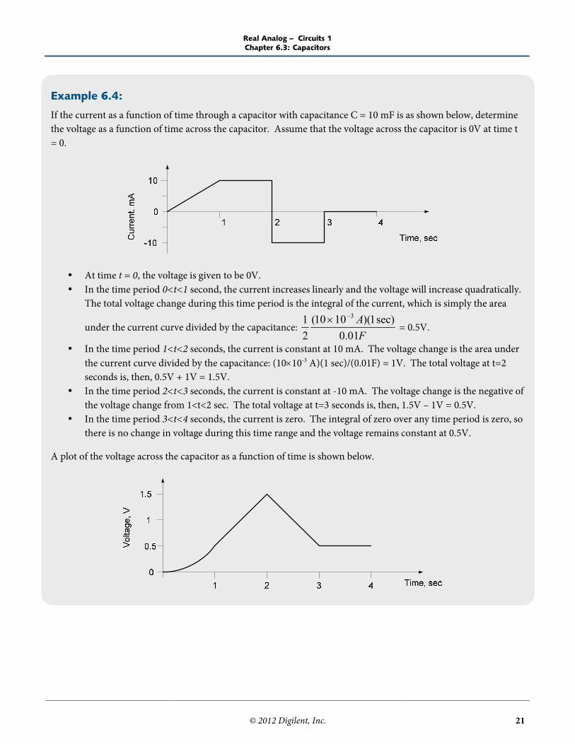
Example 6.4:

If the current as a function of time through a capacitor with capacitance C = 10 mF is as shown below, determinethe voltage as a function of time across the capacitor. Assume that the voltage across the capacitor is 0V at time t= 0.

At time t = 0, the voltage is given to be 0V. In the time period 0<t<1 second, the current increases linearly and the voltage will increase quadratically.

The total voltage change during this time period is the integral of the current, which is simply the area

under the current curve divided by the capacitance:FA01.0

sec)1)(1010(21 3

= 0.5V.

In the time period 1<t<2 seconds, the current is constant at 10 mA. The voltage change is the area underthe current curve divided by the capacitance: (1010-3 A)(1 sec)/(0.01F) = 1V. The total voltage at t=2seconds is, then, 0.5V + 1V = 1.5V.

In the time period 2<t<3 seconds, the current is constant at -10 mA. The voltage change is the negative ofthe voltage change from 1<t<2 sec. The total voltage at t=3 seconds is, then, 1.5V – 1V = 0.5V.

In the time period 3<t<4 seconds, the current is zero. The integral of zero over any time period is zero, sothere is no change in voltage during this time range and the voltage remains constant at 0.5V.

A plot of the voltage across the capacitor as a function of time is shown below.



It is often useful, when analyzing circuits containing capacitors, to examine the circuit’s response to constantoperating conditions and to instantaneous changes in operating condition. We examine the capacitor’s responseto each of these operating conditions below:

Capacitor response to constant voltage:

If the voltage across the capacitor is constant, equation (6.14) indicates that the current through thecapacitor is zero. Thus, if the voltage across the capacitor is constant, the capacitor is equivalent to a opencircuit.

This property can be extremely useful in determining a circuit’s steady-state response to constant inputs.If the inputs to a circuit change from one constant value to another, the transient components of theresponse will eventually die out and all circuit parameters will become constant. Under these conditions,capacitors can be replaced with open circuits and the circuit analyzed relatively easily. As we will see later,this operating condition can be useful in determining the response of circuits containing capacitors and indouble-checking results obtained using other methods.

Capacitor response to instantaneous voltage changes:

If the voltage across the capacitor changes instantaneously, the rate of change of voltage is infinite. Thus,by equation (6.14), if we wish to change the voltage across a capacitor instantaneously, we must supplyinfinite current to the capacitor. This implies that infinite power is available, which is not physicallypossible. Thus, in any practical circuit, the voltage across a capacitor cannot change instantaneously.

Any circuit that allows an instantaneous change in the voltage across an ideal capacitor is not physicallyrealizable. We may sometimes assume, for mathematical convenience, that an ideal capacitor’s voltagechanges suddenly; however, it must be emphasized that this assumption requires an underlyingassumption that infinite power is available and is thus not an allowable operating condition in anyphysical circuit.

Important Capacitor Properties:

Capacitors can be replaced by open-circuits, under circumstances when all operating conditions areconstant.

Voltages across capacitors cannot change instantaneously. No such requirement is placed on currents.



Energy Storage:

The power dissipated by a capacitor is

)()()( titvtp (6.16)

Since both voltage and current are functions of time, the power dissipation will also be a function of time. Thepower as a function of time is called the instantaneous power, since it provides the power dissipation at any instantin time.

Substituting equation (6.14) into equation (6.16) results in:

dttdvtvCtp )()()( (6.17)

Since power is, by definition, the rate of change of energy, the energy is the time integral of power. Integratingequation (6.17) with respect to time gives the following expression for the energy stored in a capacitor:

t tt

C CvdvCvdtdtdvCvtW )(

21)()()()()( 2

where we have set our lower limits of integration at t = - to avoid issues relative to initial conditions. We assumethat no energy is stored in the capacitor at time t = - so that

)(21)( 2 tCvtWC (6.18)

From equation (6.18) we see that the energy stored in a capacitor is always a non-negative quantity, so 0)( tWC

Ideal capacitors do not dissipate energy, as resistors do. Capacitors store energy when it is provided to them fromthe circuit; this energy can later be recovered and returned to the circuit.

Example 6.5:

Consider the circuit shown below. The voltage applied to the capacitor by the source is as shown. Plot the powerabsorbed by the capacitor and the energy stored in the capacitor as functions of time.

Power is most readily computed by taking the product of voltage and current. The current can be determinedfrom equation (6.14). The current as a function of time is plotted below.



The power absorbed by the capacitor is determined by taking a point-by-point product between the voltage andcurrent.

Recall that power is absorbed or generated based on the passive sign convention. If the relative signs betweenvoltage and current agree with the passive sign convention, the circuit element is absorbing power. If the relativesigns between voltage and current are opposite to the passive sign convention, the element is generating power.Thus, the capacitor in this example is absorbing power for the first microsecond. It generates power (returnspower to the voltage source) during the second microsecond). After the second microsecond, the current is zeroand the capacitor neither absorbs nor generates power.

The energy stored in the capacitor can be determined either from integrating the power or from application ofequation (6.18) to the voltage curve provided in the problem statement. The energy in the capacitor as a functionof time is shown below:

WC(t),J

During the first microsecond, while the capacitor is absorbing power, the energy in the capacitor is increasing.The maximum energy in the capacitor is 50 J, at 1s. During the second microsecond, the capacitor is releasingpower back to the circuit and the energy in the capacitor is decreasing. At 2s, the capacitor still has 12.5 J ofstored energy. After 2s, the capacitor neither absorbs nor generates energy and the energy stored in thecapacitor remains at 12.5J.



Capacitors in Series:

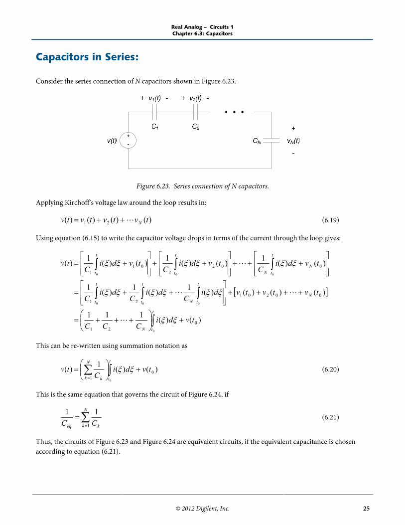
Consider the series connection of N capacitors shown in Figure 6.23.

Figure 6.23. Series connection of N capacitors.

Applying Kirchoff’s voltage law around the loop results in:

)()()()( 21 tvtvtvtv N (6.19)

Using equation (6.15) to write the capacitor voltage drops in terms of the current through the loop gives:

)()(111

)()()()(1)(1)(1

)()(1)()(1)()(1)(

021

0020121

0022

011

0

000

000

tvdiCCC

tvtvtvdiC

diC

diC

tvdiC

tvdiC

tvdiC

tv

t

tN

N

t

tN

t

t

t

t

N

t

tN

t

t

t

t

This can be re-written using summation notation as

)()(1)( 01

0

tvdiC

tvt

t

N

k k

(6.20)

This is the same equation that governs the circuit of Figure 6.24, if

N

k keq CC 1

11(6.21)

Thus, the circuits of Figure 6.23 and Figure 6.24 are equivalent circuits, if the equivalent capacitance is chosenaccording to equation (6.21).



Figure 6.24. Equivalent circuit to Figure 3.

For the special case of two capacitors C1 and C2 in series, equation (6.21) simplifies to

21

21

CCCC

Ceq (6.22)

Equations (6.21) and (6.22) are analogous to the equations, which provide the equivalent resistance of parallelcombinations of resistors.

Capacitors in Parallel:

Consider the parallel combination of N capacitors, as shown in Figure 6.25.

Figure 6.25. Series connection of N capacitors.

Applying Kirchoff’s current law at the upper node results in:

)()()()( 21 titititi N (6.23)

Using equation (6.14) to write the capacitor currents in terms of their voltage drop gives:

dttdvCCC

dttdvC

dttdvC

dttdvCti

N

N

)(

)()()()(

21

21



Using summation notation results in

dttdvCti

N

kk

)()(1

(6.24)


N

kkeq CC

1(6.25)

Thus, the equivalent capacitance of a parallel combination of capacitors is simply the sum of the individualcapacitances. This result is analogous to the equations, which provide the equivalent resistance of a seriescombination of resistors.


Summary: Series and Parallel Capacitors The equivalent capacitance of a series combination of capacitors C1, C2, …, CN is governed by a relation

which is analogous to that providing the equivalent resistance of a parallel combination of resistors:

N

k keq CC 1

11

The equivalent capacitance of a parallel combination of capacitors C1, C2, …, CN is governed by a relationwhich is analogous to that providing the equivalent resistance of a series combination of resistors:

N

kkeq CC

1

Practical Capacitors:

Commercially available capacitors are manufactured in a wide range of both conductor and dielectric materialsand are available in a wide range of capacitances and voltage ratings. The voltage rating of the device is themaximum voltage, which can be safely applied to the capacitor; using voltages higher than the rated value will



damage the capacitor. The capacitance of commercially available capacitors is commonly measured in micro-farads (F; one microfarad is 10-6 of a Farad) or pico-farads (pF; one picofarad is 10-12 of a Farad). Largecapacitors are available, but are relatively infrequently used. These are generally called “super-capacitors” or“ultra-capacitors” and are available in capacitances up to tens of Farads. For most applications, however, usingone would be comparable to buying a car with a 1000 gallon gas tank.

Several approaches are used for labeling a capacitor with its capacitance value. Large capacitors often have theirvalue printed plainly on them, such as "10 uF" (for 10 microfarads). Smaller capacitors, appearing as small disks orwafers, often have their values printed on them in an encoded manner. For these capacitors, a three digit numberindicates the capacitor value in pico-farads. The first two digits provides the "base" number, and the third digitprovides an exponent of 10 (so, for example, "104" printed on a capacitor indicates a capacitance value of 10 x 104

or 100000 pF). Occasionally, a capacitor will only show a two digit number, in which case that number is simplythe capacitor value in pF. (For completeness, if a capacitor shows a three digit number and the third digit is 8 or 9,then the first two digits are multiplied by .01 and .1 respectively).

Capacitors are generally classified according to the dielectric material used. Common capacitor types includemica, ceramic, Mylar, paper, Teflon and polystyrene. An important class of capacitors which require specialmention are electrolytic capacitors. Electrolytic capacitors have relatively large capacitances relative to other typesof capacitors of similar size. However, some care must be exercised when using electrolytic capacitors – they arepolarized and must be connected to a circuit with the correct polarity. The positive lead of the capacitor must beconnected to the positive lead of the circuit. Connecting the positive lead of the capacitor to the negative lead of acircuit can result in unwanted current “leakage” through the capacitor or, in extreme cases, destroy the capacitor.Polarized capacitors either have a dark stripe near the pin that must be kept at the higher voltage, or a "-" near thepin that must be kept at a lower voltage.

Practical capacitors, unlike ideal capacitors, will dissipate some power. This power loss is primarily due to leakagecurrents. These currents are due to the fact that real dielectric materials are not perfect insulators – some smallcurrent will tend to flow through them. The overall effect is comparable to placing a high resistance in parallelwith an ideal capacitor, as shown in Figure 6.27. Different types of capacitors have different leakage currents.Mica capacitors tend to have low leakage currents, the leakage currents of ceramic capacitors vary according to thetype of capacitor, and electrolytic capacitors have high leakage currents.

Figure 6.27. Model of practical capacitor including leakage current path.



Section Summary:

Capacitors store electrical energy. This energy is stored in an electric field between two conductive elements,separated by an insulating material.

Capacitor energy storage is dependent upon the voltage across the capacitor, if the capacitor voltage is known,the energy in the capacitor is known.

The voltage-current relationship for a capacitor is:

dttdvCti )()(

where C is the capacitance of the capacitor. Units of capacitance are Farads (abbreviated F). The capacitanceof a capacitor, very roughly speaking, gives an indication of how much energy it can store.

The above voltage-current relation results in the following important properties of capacitors:1. If the capacitor voltage is constant, the current through the capacitor is zero. Thus, if the capacitor

voltage is constant, the capacitor can be modeled as an open circuit.2. Changing the capacitor voltage instantaneously requires infinite power. Thus (for now, anyway) we will

assume that capacitors cannot instantaneously change their voltage. Capacitors placed in series or parallel with one another can be modeled as a single equivalent capacitance.

Thus, capacitors in series or in parallel are not “independent” energy storage elements.

Exercises:

1. Determine the maximum and minimum capacitances that can be obtained from four 1F capacitors. Sketchthe circuit schematics that provide these capacitances.

2. Determine voltage divider relationships to provide v1 and v2 for the two uncharged series capacitors shownbelow. Use your result to determine v2 if C1 = C2 = 10F.

Real Analog – Circuits 1Chapter 6.4: Inductors


6.4: InductorsWe continue our study of energy storage elements with a discussion of inductors. Inductors, like resistors andcapacitors, are passive two-terminal circuit elements. That is, no external power supply is necessary to make themfunction. Inductors commonly consist of a conductive wire wrapped around a core material; inductors storeenergy in the form of a magnetic field set up around the current-carrying wire.

In this section, we describe physical properties of inductors and provide a mathematical model for an idealinductor. Using this ideal inductor model, we will develop mathematical relationships for the energy stored in aninductor and governing relations for series and parallel connections of inductors. The section concludes with abrief discussion of practical (non-ideal) inductors.

Inductors:

Passing a current through a conductive wire will create a magnetic field around the wire. This magnetic field isgenerally thought of in terms of as forming closed loops of magnetic flux around the current-carrying element.This physical process is used to create inductors. Figure 6.28 illustrates a common type of inductor, consisting of acoiled wire wrapped around a core material. Passing a current through the conducting wire sets up lines ofmagnetic flux, as shown in Figure 6.28; the inductor stores energy in this magnetic field. The inductance of theinductor is a quantity, which tells us how much energy can be stored by the inductor. Higher inductance meansthat the inductor can store more energy. Inductance has units of Henrys, abbreviated H.

The amount of inductance an inductor has is governed by the geometry of the inductor and the properties of thecore material. These effects can be complex; rather than attempt a comprehensive discussion of these effects, wewill simply claim that, in general, inductance is dependent upon the following parameters:

The number of times the wire is wrapped around the core. More coils of wire results in a higherinductance.

The core material’s type and shape. Core materials are commonly ferromagnetic materials, since theyresult in higher magnetic flux and correspondingly higher energy storage. Air, however, is a fairlycommonly used core material – presumably because of its ready availability.

The spacing between turns of the wire around the core.



Figure 6.28. Wire-wrapped inductor with applied current through conductive wire.

We will denote the total magnetic flux created by the inductor by , as shown in Figure 6.28. For a linearinductor, the flux is proportional to the current passing through the wound wires. The constant ofproportionality is the inductance, L:

)()( tLit (6.26)

Voltage is the time rate of change of magnetic flux, so

dttdtv )()(

(6.27)

Combining equations (6.26) and (6.27) results in the voltage-current relationship for an ideal inductor:

dttdiLtv )()( (6.28)

The circuit symbol for an inductor is shown in Figure 6.29, along with the sign conventions for the voltage-current relationship of equation (6.28). The passive sign convention is used in the voltage-current relationship, sopositive current is assumed to enter the terminal with positive voltage polarity.

Figure 6.29. Inductor circuit symbol and voltage-current sign convention.



Integrating both sides of equation (6.28) results in the following form for the inductor’s voltage-currentrelationship:

)()(1)( 0

0

tidvL

tit

t

(6.29)

In equation (6.29), i(t0) is a known current at some initial time t0 and is used as a dummy variable of integrationto emphasize that the only “t” which survives the integration process is the upper limit of the integral.

Important result:

The voltage-current relationship for an ideal inductor can be stated in either differential or integral form, asfollows:

dttdiLtv )()(

)()(1)( 0

0

tidvL

tit

t

Example 6.6:

A circuit contains a 100mH inductor. The current as a function of time through the inductor is measured andshown below. Plot the voltage across the inductor as a function of time.

In the time range 0<t<1ms, the rate of change of current is 10 A/sec. Thus, from equation (3), the voltageis )/10)(1.0()( sAHtv = 1V.

In the time range 1ms<t<2ms, the rate of change of current is -5A/sec. The voltage is -0.5V. In the time range 2ms<t<3ms, the current is constant and there is no voltage across the inductor. In the time range 3ms<t<5ms, the rate of change of current is -5A/sec. The voltage is -0.5V.



The plot of voltage vs. time is shown below:

Power is the product of voltage and current. If the signs of voltage and current are the same according to thepassive sign convention, the circuit element absorbs power. If the signs of voltage and current are not the same,the circuit element generates power. From the above voltage and current curves, the inductor is absorbing powerfrom the circuit during the times 0<t<1ms and 4ms<t<5ms. The inductor returns power to the circuit during thetimes 1ms<t<2ms and 3ms<t<4ms.

Time, msec

0

-5

10

1 2 3 4 5

5

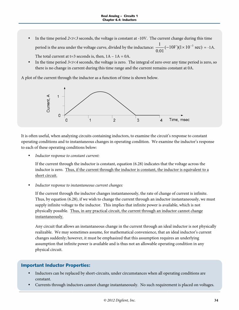
Example 2: If the voltage as a function of time across an inductor with inductance L = 10 mH is as shown below,determine the current as a function of time through the capacitor. Assume that the current through the capacitoris 0A at time t = 0.

At time t = 0, the current is given to be 0A. In the time period 0<t<1 msec, the voltage is constant and positive so the current will increase linearly.

The total current change during this time period is the area under the voltage curve curve, divided by the

inductance: sec)101)(10(01.01 3V = 1A.

In the time period 1<t<2 msec, the voltage is decreasing linearly. The current during this time period is aquadratic curve, concave downward. The maximum value of current is 1.25A, at t = 1.5 msec. Thecurrent at the end of this time period is 1A.



In the time period 2<t<3 seconds, the voltage is constant at -10V. The current change during this time

period is the area under the voltage curve, divided by the inductance: sec)101)(10(01.01 3 V = -1A.

The total current at t=3 seconds is, then, 1A – 1A = 0A. In the time period 3<t<4 seconds, the voltage is zero. The integral of zero over any time period is zero, so

there is no change in current during this time range and the current remains constant at 0A.

A plot of the current through the inductor as a function of time is shown below.

It is often useful, when analyzing circuits containing inductors, to examine the circuit’s response to constantoperating conditions and to instantaneous changes in operating condition. We examine the inductor’s responseto each of these operating conditions below:

Inductor response to constant current:

If the current through the inductor is constant, equation (6.28) indicates that the voltage across theinductor is zero. Thus, if the current through the inductor is constant, the inductor is equivalent to ashort circuit.

Inductor response to instantaneous current changes:

If the current through the inductor changes instantaneously, the rate of change of current is infinite.Thus, by equation (6.28), if we wish to change the current through an inductor instantaneously, we mustsupply infinite voltage to the inductor. This implies that infinite power is available, which is notphysically possible. Thus, in any practical circuit, the current through an inductor cannot changeinstantaneously.

Any circuit that allows an instantaneous change in the current through an ideal inductor is not physicallyrealizable. We may sometimes assume, for mathematical convenience, that an ideal inductor’s currentchanges suddenly; however, it must be emphasized that this assumption requires an underlyingassumption that infinite power is available and is thus not an allowable operating condition in anyphysical circuit.

Important Inductor Properties:

Inductors can be replaced by short-circuits, under circumstances when all operating conditions areconstant.

Currents through inductors cannot change instantaneously. No such requirement is placed on voltages.



Energy Storage:

The instantaneous power dissipated by an electrical circuit element is the product of the voltage and current:

)()()( titvtp (6.30)

Using equation (6.28) to write the voltage in equation (6.30) in terms of the inductor’s current:

dttditiLtp )()()( (6.31)

As was previously done for capacitors, we integrate the power with respect to time to get the energy stored in theinductor:

t

L dtdtdiLitW )()()(

Which, after some manipulation (comparable to the approach taken when we calculated energy storage incapacitors), results in the following expression for the energy stored in an inductor:

)(21)( 2 tLitWL (6.32)

Inductors in Series:

Consider the series connection of N inductors shown in Figure 6.30.

Figure 6.30. Series connection of N inductors.

Applying Kirchoff’s voltage law around the loop results in:

)()()()( 21 tvtvtvtv N (6.33)



Using equation (6.28) to write the inductor voltage drops in terms of the current through the loop gives:

dttdiLLL

dttdiL

dttdiL

dttdiLtv

N

N

)(

)()()()(

21

21

Using summation notation results in

dttdiLtv

N

kk

)()(1

(6.34)


N

kkeq LL

1(6.35)

Thus, the equivalent inductance of a series combination of inductors is simply the sum of the individualinductances. This result is analogous to the equations which provide the equivalent resistance of a seriescombination of resistors.


Inductors in Parallel:

Consider the parallel combination of N inductors, as shown in Figure 6.32.

Figure 6.32. Parallel combination of I inductors.



Applying Kirchoff’s current law at the upper node results in:

)()()()( 21 titititi N (6.36)

Using equation (6.29) to write the inductor currents in terms of their voltage drops gives:

)()(111

)()()()(1)(1)(1

)()(1)()(1)()(1)(

021

0020121

0022

011

0

000

000

tidvLLL

tititidvL

dvL

dvL

tidvL

tidvL

tidvL

ti

t

tN

N

t

tN

t

t

t

t

N

t

tN

t

t

t

t

This can be re-written using summation notation as

)()(1)( 01

0

tidvL

tit

t

N

k k

(6.37)


N

k keq LL 1

11(6.38)

For the special case of two inductors L1 and L2 in series, equation (13) simplifies to

21

21

LLLL

Leq (6.39)

Equations (6.38) and (6.39) are analogous to the equations which provide the equivalent resistance of parallelcombinations of resistors.

Summary: Series and Parallel Inductors

The equivalent inductance of a series combination of inductors L1, L2, …, LN is governed by a relationwhich is analogous to that providing the equivalent resistance of a series combination of resistors:

N

kkeq LL

1

The equivalent inductance of a parallel combination of inductors L1, L2, …, LN is governed by a relationwhich is analogous to that providing the equivalent resistance of a parallel combination of resistors:

N

k keq LL 1

11



Practical Inductors:

Most commercially available inductors are manufactured by winding wire in various coil configurations around acore. Cores can be a variety of shapes; Figure 6.28 in this chapter shows a core, which is basically a cylindrical bar.Toroidal cores are also fairly common – a closely wound toroidal core has the advantage that the magnetic field isconfined nearly entirely to the space inside the winding.

Inductors are available with values from less than 1 micro-Henry (1H = 10-6 Henries) up to tens of Henries. A1H inductor is very large; inductances of most commercially available inductors are measured in millihenries(1mH = 10-3 Henries) or microhenries. Larger inductors are generally used for low-frequency applications (inwhich the signals vary slowly with time).

Attempts at creating inductors in integrated-circuit form have been largely unsuccessful; therefore many circuitsthat are implemented as integrated circuits do not include inductors. Inclusion of inductance in the analysis stageof these circuits may however, be important. Since any current-carrying conductor will create a magnetic field,the stray inductance of supposedly non-inductive circuit elements can become an important consideration in theanalysis and design of a circuit.

Practical inductors, unlike the ideal inductors discussed in this chapter, dissipate power. An equivalent circuitmodel for a practical inductor is generally created by placing a resistance in series with an ideal inductor, as shownin Figure 6.33.

Figure 6.33. Equivalent circuit model for a practical inductor.



Section Summary:

Inductors store magnetic energy. This energy is stored in a magnetic field (typically) generated by a coiledwire wrapped around a core material.

Inductor energy storage is dependent upon the current through the inductor, if the inductor current is known,the energy in the inductor is known.

The voltage-current relationship for an inductor is:

dttdiLtv )()(

where L is the inductance of the inductor. Units of inductance are Henries (abbreviated H). The inductanceof an inductor, very roughly speaking, gives an indication of how much energy it can store.

The above voltage-current relation results in the following important properties of inductors:1. If the inductor current is constant, the voltage across the inductor is zero. Thus, if the inductor current is

constant, the inductor can be modeled as a short circuit.2. Changing the inductor current instantaneously requires infinite power. Thus (for now, anyway) we will

assume that inductors cannot instantaneously change their current. Inductors placed in series or parallel with one another can be modeled as a single equivalent inductance.

Thus, inductors in series or in parallel are not “independent” energy storage elements.

Exercises:

1. Determine the equivalent inductance of the network below:

6. introduction and chapter objectives - digilentinc · ©2012 digilent,inc. 1 6. introduction and...

Documents