6 graphing systems of linear inequalities in two variables linear programming problems graphical...
TRANSCRIPT

6 6 Graphing Systems of Linear Graphing Systems of Linear
Inequalities in Two VariablesInequalities in Two Variables
Linear Programming ProblemsLinear Programming Problems
Graphical Solutions of Linear Graphical Solutions of Linear Programming ProblemsProgramming Problems
The Simplex Method: The Simplex Method: Standard Maximization ProblemsStandard Maximization Problems
The Simplex Method: The Simplex Method: Standard Minimization ProblemsStandard Minimization Problems
Linear Programming: A Geometric ApproachLinear Programming: A Geometric Approach
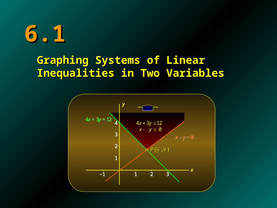
6.16.1Graphing Systems of Linear Inequalities Graphing Systems of Linear Inequalities in Two Variablesin Two Variables
xx
yy
44xx + 3+ 3yy = = 1212
12 127 7( , )P 12 127 7( , )P
xx –– y y = = 00
4 3 120
x yx y
4 3 120
x yx y
44
33
22
11
–– 11 11 22 33

Graphing Linear InequalitiesGraphing Linear Inequalities
We’ve seen that We’ve seen that a linear a linear equationequation in two variables in two variables x x and and y y
has a has a solution setsolution set that may be exhibited that may be exhibited graphicallygraphically as as points points on a straight lineon a straight line in the in the xyxy-plane-plane..
There is also a simple There is also a simple graphical representationgraphical representation for for linear linear inequalitiesinequalities of two variables of two variables::
0ax by c 0ax by c
0ax by c 0ax by c
0ax by c 0ax by c
0ax by c 0ax by c
0ax by c 0ax by c

Procedure for Graphing Linear InequalitiesProcedure for Graphing Linear Inequalities
1.1. Draw the Draw the graphgraph of the of the equationequation obtained for the given obtained for the given inequality by inequality by replacing the inequality sign with an replacing the inequality sign with an equal signequal sign..✦ Use a Use a dashed or dotted linedashed or dotted line if the problem involves a if the problem involves a
strict inequalitystrict inequality, , << or or >>..✦ Otherwise, use a Otherwise, use a solid linesolid line to indicate that to indicate that the line the line
itself constitutes part of the solutionitself constitutes part of the solution..2.2. Pick a test pointPick a test point lying in one of the half-planes lying in one of the half-planes
determined by the line sketched in determined by the line sketched in step 1step 1 and and substitutesubstitute the values of the values of xx and and yy into the given into the given inequalityinequality..✦ Use the Use the originorigin whenever possible. whenever possible.
3.3. If the If the inequality is satisfiedinequality is satisfied, the graph of , the graph of the inequality the inequality includes the half-planeincludes the half-plane containing the containing the test pointtest point..✦ Otherwise, the solution includes the half-plane not Otherwise, the solution includes the half-plane not
containing the test point.containing the test point.

ExamplesExamples
Determine the Determine the solution setsolution set for the for the inequalityinequality 22xx + 3 + 3yy 6 6..SolutionSolution ReplacingReplacing the the inequalityinequality with an with an equalityequality ==, we obtain , we obtain
the equation the equation 22xx + 3 + 3yy = 6 = 6, whose graph is:, whose graph is:
xx
yy
77
55
33
11
–– 1 1 –– 55 –– 33 – – 11 11 33 55
22xx + 3 + 3yy = 6 = 6

ExamplesExamples
Determine the Determine the solution setsolution set for the for the inequalityinequality 22xx + 3 + 3yy 6 6..SolutionSolution Picking the Picking the originorigin as a as a test pointtest point, we find , we find 2(0) + 3(0) 2(0) + 3(0) 6 6, ,
or or 0 0 6 6, which is , which is falsefalse. . Thus, the Thus, the solution setsolution set is: is:
xx
yy
77
55
33
11
–– 1 1 –– 55 –– 33 – – 11 11 33 55
22xx + 3 + 3yy = 6 = 622xx + 3 + 3yy 6 6
(0, 0)(0, 0)

Graphing Systems of Linear InequalitiesGraphing Systems of Linear Inequalities
The The solution setsolution set of a of a system of linear inequalitiessystem of linear inequalities in two in two variables variables x x and and yy is the is the set of all pointsset of all points ((xx, , yy)) that that satisfy satisfy each inequalityeach inequality of the system. of the system.
The The graphical solutiongraphical solution of such a system may be obtained of such a system may be obtained by by graphing the solution set for each inequalitygraphing the solution set for each inequality independently and then independently and then determining the region in determining the region in commoncommon with each solution set. with each solution set.
–– 5 5 – – 33 11 33 55
ExamplesExamples
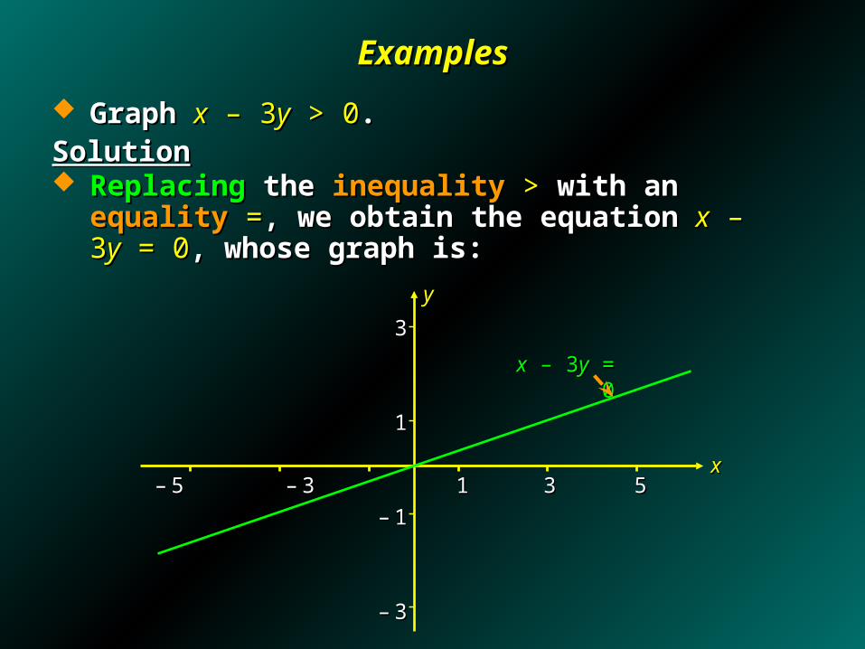
Graph Graph xx – 3 – 3yy > 0 > 0..SolutionSolution ReplacingReplacing the the inequalityinequality >> with an with an equalityequality ==, we obtain , we obtain
the equation the equation xx – 3 – 3yy = 0 = 0, whose graph is:, whose graph is:
xx
yy
33
11
–– 11
–– 3 3
xx – 3 – 3yy = 0 = 0
ExamplesExamples
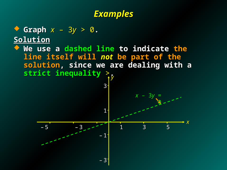
Graph Graph xx – 3 – 3yy > 0 > 0..SolutionSolution We use a We use a dashed linedashed line to indicate to indicate the line itself will the line itself will notnot be be
part of the solutionpart of the solution, since we are dealing with a , since we are dealing with a strict strict inequalityinequality >>. .
xx
yy
xx – 3 – 3yy = 0 = 0
–– 5 5 – – 33 11 33 55
33
11
–– 11
–– 3 3
–– 5 5 – – 33 11 33 55
33
11
–– 11
–– 3 3
ExamplesExamples
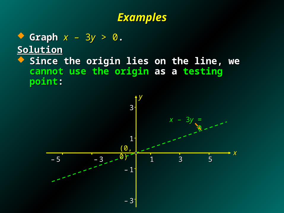
Graph Graph xx – 3 – 3yy > 0 > 0..SolutionSolution Since the origin lies on the line, we Since the origin lies on the line, we cannot use the origincannot use the origin
as a as a testing pointtesting point: :
xx
yy
xx – 3 – 3yy = 0 = 0
(0, 0)(0, 0)

ExamplesExamples
Graph Graph xx – 3 – 3yy > 0 > 0..SolutionSolution Picking instead Picking instead (3, 0)(3, 0) as a as a test pointtest point, we find , we find (3) – 2(0) > 0(3) – 2(0) > 0, ,
or or 3 > 03 > 0, which is , which is truetrue. . Thus, the Thus, the solution setsolution set is: is:
yy
xx – 3 – 3yy = 0 = 0
xx – 3 – 3yy > 0 > 0
–– 5 5 – – 33 11 33 55
33
11
–– 11
–– 3 3
xx(3, 0)(3, 0)

Graphing Systems of Linear InequalitiesGraphing Systems of Linear Inequalities
The The solution setsolution set of a of a system of linear inequalitiessystem of linear inequalities in two in two variables variables x x and and yy is the is the set of all pointsset of all points ((xx, , yy)) that that satisfy satisfy each inequalityeach inequality of the system. of the system.
The The graphical solutiongraphical solution of such a system may be obtained of such a system may be obtained by by graphing the solution set for each inequalitygraphing the solution set for each inequality independently and then independently and then determining the region in determining the region in commoncommon with each solution set. with each solution set.
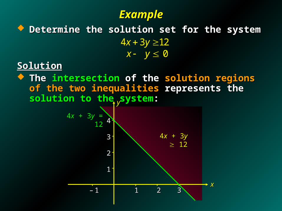
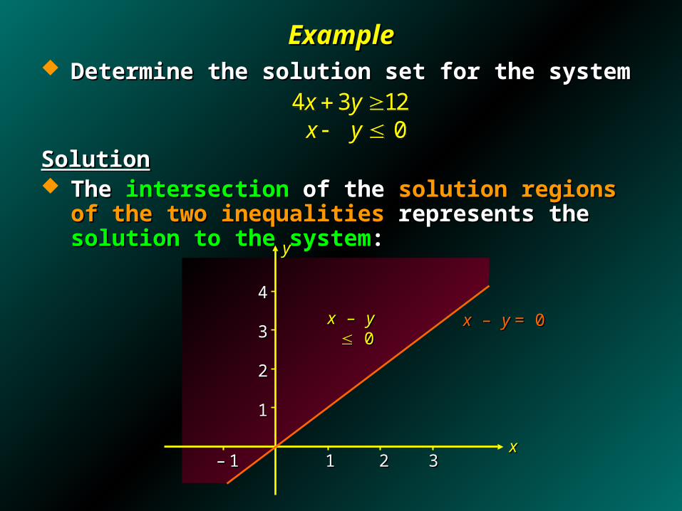
ExampleExample Determine the solution set for the systemDetermine the solution set for the system
SolutionSolution The The intersectionintersection of the of the solution regionssolution regions of the two of the two
inequalitiesinequalities represents the represents the solution to the systemsolution to the system::
4 3 120
x yx y
4 3 120
x yx y
xx
yy
44
33
22
11
44xx + 3 + 3yy 12 12
44xx + 3 + 3yy = 12 = 12
–– 11 11 22 33
ExampleExample Determine the solution set for the systemDetermine the solution set for the system
SolutionSolution The The intersectionintersection of the of the solution regionssolution regions of the two of the two
inequalitiesinequalities represents the represents the solution to the systemsolution to the system::
4 3 120
x yx y
4 3 120
x yx y
xx
yy
xx – – y y 0 0 xx – – y y = 0= 0
44
33
22
11
–– 11 11 22 33

ExampleExample Determine the solution set for the systemDetermine the solution set for the system
SolutionSolution The The intersectionintersection of the of the solution regionssolution regions of the two of the two
inequalitiesinequalities represents the represents the solution to the systemsolution to the system::
4 3 120
x yx y
4 3 120
x yx y
xx
yy
44xx + 3 + 3yy = 12 = 12
xx – – y y = 0= 0
4 3 120
x yx y
4 3 120
x yx y
44
33
22
11
–– 11 11 22 33
12 127 7( , )P 12 127 7( , )P

Bounded and Unbounded SetsBounded and Unbounded Sets
The The solution setsolution set of a system of linear inequalities of a system of linear inequalities is is boundedbounded if it if it can be enclosed by a circlecan be enclosed by a circle..
Otherwise, it is Otherwise, it is unboundedunbounded..
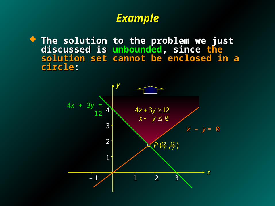
ExampleExample
The solution to the problem we just discussed is The solution to the problem we just discussed is unboundedunbounded, since , since the solution setthe solution set cannot be cannot be enclosed in a circleenclosed in a circle::
xx
yy
44xx + 3 + 3yy = 12 = 12
12 127 7( , )P 12 127 7( , )P
xx – – y y = 0= 0
4 3 120
x yx y
4 3 120
x yx y
44
33
22
11
–– 11 11 22 33

77
55
33
11
––1 1 11 33 55 99
ExampleExample Determine the solution set for the systemDetermine the solution set for the system
SolutionSolution The The intersectionintersection of the of the solution regionssolution regions of the four of the four
inequalitiesinequalities represents the represents the solution to the systemsolution to the system::
6 0 2 8 0 0 0 x y x y x y 6 0 2 8 0 0 0 x y x y x y
xx
yy
2 8 0x y 2 8 0x y
6 0x y 6 0x y
(2,4)P(2,4)P
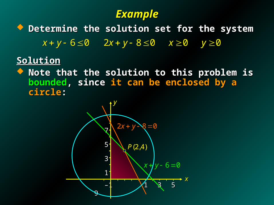
ExampleExample Determine the solution set for the systemDetermine the solution set for the system
SolutionSolution Note that the solution to this problem is Note that the solution to this problem is boundedbounded, since , since it it
can be enclosed by a circlecan be enclosed by a circle::
6 0 2 8 0 0 0 x y x y x y 6 0 2 8 0 0 0 x y x y x y
––1 1 11 33 55 99xx
yy
77
55
33
116 0x y 6 0x y
(2,4)P(2,4)P
2 8 0x y 2 8 0x y

6.26.2Linear Programming ProblemsLinear Programming Problems
0
0
x
y
0
0
x
y
1.2P x y 1.2P x y
3 300x y 3 300x y
2 180x y 2 180x y
Maximize
Subject to

Linear Programming ProblemLinear Programming Problem
A linear programming problem consists of a A linear programming problem consists of a linear objective functionlinear objective function to be to be maximized or maximized or minimizedminimized subject to certain subject to certain constraintsconstraints in the in the form of form of linear equations or inequalitieslinear equations or inequalities..

Applied Example 1:Applied Example 1: A Production Problem A Production Problem
Ace Novelty wishes to produce Ace Novelty wishes to produce two types of souvenirstwo types of souvenirs: : type-A type-A will result in a profit of will result in a profit of $1.00$1.00, and , and type-Btype-B in a in a profit of profit of $1.20$1.20..
To manufacture a To manufacture a type-Atype-A souvenir requires souvenir requires 2 2 minutes on minutes on machine Imachine I and and 11 minute on minute on machine IImachine II..
A A type-Btype-B souvenir requires souvenir requires 11 minute on minute on machine Imachine I and and 3 3 minutes on minutes on machine IImachine II..
There are There are 33 hours available on hours available on machine Imachine I and and 5 5 hours hours available on available on machine IImachine II..
How many souvenirsHow many souvenirs of each type should Ace make in of each type should Ace make in order to order to maximize its profitmaximize its profit??

Applied Example 1:Applied Example 1: A Production Problem A Production Problem
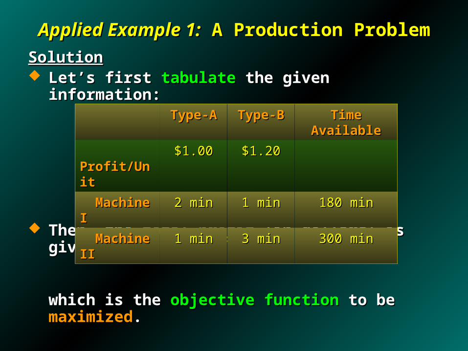
SolutionSolution Let’s first Let’s first tabulatetabulate the given information: the given information:
Let Let xx be the number of be the number of type-A type-A souvenirs and souvenirs and yy the number the number of of type-Btype-B souvenirs to be made. souvenirs to be made.
Type-AType-A Type-BType-B Time AvailableTime Available
Profit/UnitProfit/Unit $1.00$1.00 $1.20$1.20
Machine IMachine I 2 min2 min 1 min1 min 180 min180 min
Machine IIMachine II 1 min1 min 3 min3 min 300 min300 min
Applied Example 1:Applied Example 1: A Production Problem A Production Problem
SolutionSolution Let’s first Let’s first tabulatetabulate the given information: the given information:
Then, the Then, the total profittotal profit (in dollars) is given by (in dollars) is given by
which is the which is the objective functionobjective function to be to be maximizedmaximized..
1.2P x y 1.2P x y
Type-AType-A Type-BType-B Time AvailableTime Available
Profit/UnitProfit/Unit $1.00$1.00 $1.20$1.20
Machine IMachine I 2 min2 min 1 min1 min 180 min180 min
Machine IIMachine II 1 min1 min 3 min3 min 300 min300 min
Applied Example 1:Applied Example 1: A Production Problem A Production Problem
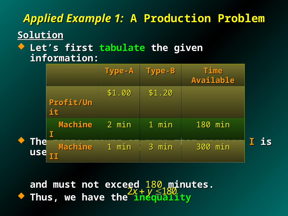
SolutionSolution Let’s first Let’s first tabulatetabulate the given information: the given information:
The total amount of The total amount of timetime that that machine Imachine I is used is is used is
and must not exceed and must not exceed 180180 minutes. minutes. Thus, we have the Thus, we have the inequalityinequality
2x y2x y
2 180x y 2 180x y
Type-AType-A Type-BType-B Time AvailableTime Available
Profit/UnitProfit/Unit $1.00$1.00 $1.20$1.20
Machine IMachine I 2 min2 min 1 min1 min 180 min180 min
Machine IIMachine II 1 min1 min 3 min3 min 300 min300 min
Applied Example 1:Applied Example 1: A Production Problem A Production Problem
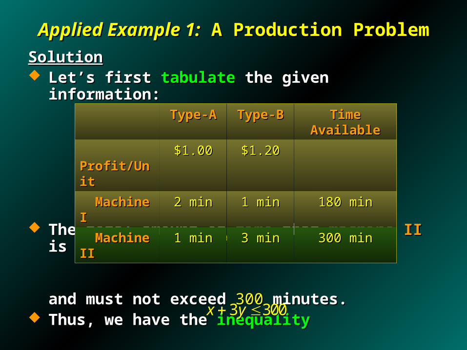
SolutionSolution Let’s first Let’s first tabulatetabulate the given information: the given information:
The total amount of The total amount of timetime that that machine IImachine II is used is is used is
and must not exceed and must not exceed 300300 minutes. minutes. Thus, we have the Thus, we have the inequalityinequality
3x y3x y
3 300x y 3 300x y
Type-AType-A Type-BType-B Time AvailableTime Available
Profit/UnitProfit/Unit $1.00$1.00 $1.20$1.20
Machine IMachine I 2 min2 min 1 min1 min 180 min180 min
Machine IIMachine II 1 min1 min 3 min3 min 300 min300 min
Applied Example 1:Applied Example 1: A Production Problem A Production Problem
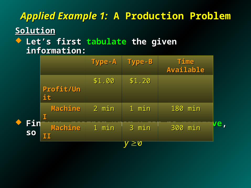
SolutionSolution Let’s first Let’s first tabulatetabulate the given information: the given information:
Finally, neither Finally, neither x x nor nor yy can be can be negativenegative, so, so
0
0
x
y
0
0
x
y
Type-AType-A Type-BType-B Time AvailableTime Available
Profit/UnitProfit/Unit $1.00$1.00 $1.20$1.20
Machine IMachine I 2 min2 min 1 min1 min 180 min180 min
Machine IIMachine II 1 min1 min 3 min3 min 300 min300 min

Applied Example 1:Applied Example 1: A Production Problem A Production Problem
SolutionSolution In short, we want to In short, we want to maximizemaximize the the objective functionobjective function
subject tosubject to the the system of inequalitiessystem of inequalities
We will discuss the We will discuss the solutionsolution to this problem in to this problem in section 6.4section 6.4..
0
0
x
y
0
0
x
y
1.2P x y 1.2P x y
3 300x y 3 300x y
2 180x y 2 180x y

Applied Example 2:Applied Example 2: A Nutrition Problem A Nutrition Problem
A nutritionist advises an individual who is suffering from A nutritionist advises an individual who is suffering from ironiron and and vitamin B vitamin B deficiency to take at least deficiency to take at least 24002400 milligrams (mg) of milligrams (mg) of ironiron, , 21002100 mg of mg of vitamin Bvitamin B11, and , and 15001500
mg of mg of vitamin Bvitamin B22 over a period of time. over a period of time.
Two vitamin pills are suitable, Two vitamin pills are suitable, brand-Abrand-A and and brand-Bbrand-B.. Each Each brand-Abrand-A pill costs pill costs 66 cents and contains cents and contains 4040 mg of mg of ironiron, ,
1010 mg of mg of vitamin Bvitamin B11, and , and 55 mg of mg of vitamin Bvitamin B22..
Each Each brand-B brand-B pill costs pill costs 88 cents and contains cents and contains 1010 mg of mg of ironiron and and 1515 mg each of mg each of vitamins Bvitamins B11 and and BB22..
What combination of pillsWhat combination of pills should the individual purchase should the individual purchase in order to in order to meetmeet the minimum iron and vitamin the minimum iron and vitamin requirementsrequirements at the at the lowest costlowest cost??
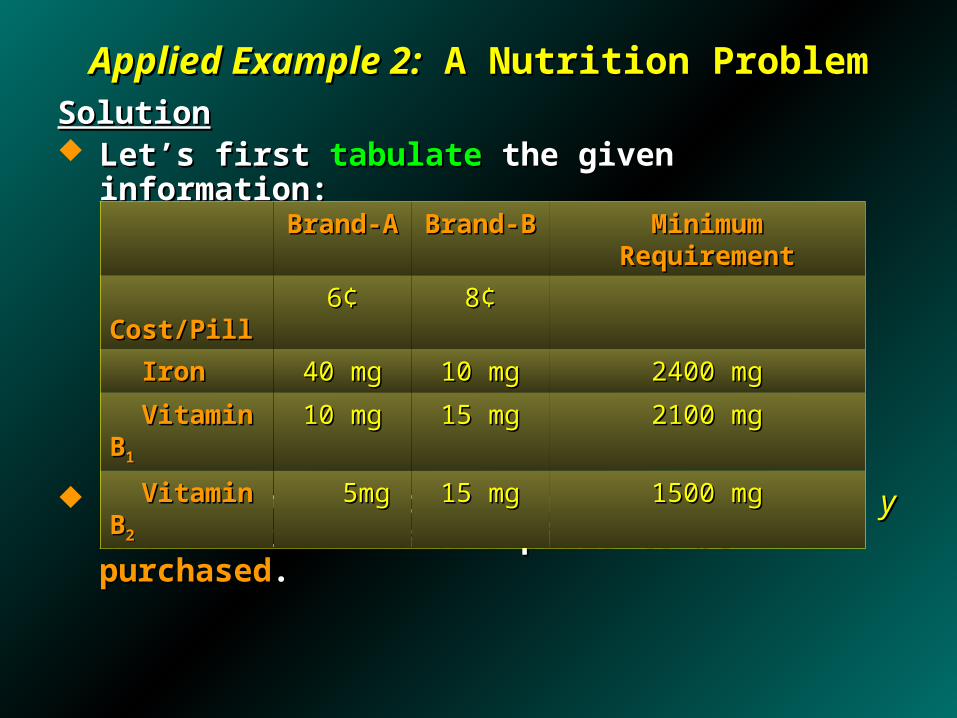
Applied Example 2:Applied Example 2: A Nutrition Problem A Nutrition ProblemSolutionSolution Let’s first Let’s first tabulatetabulate the given information: the given information:
Let Let xx be the number of be the number of brand-A brand-A pills and pills and yy the number of the number of brand-Bbrand-B pills to be pills to be purchasedpurchased..
Brand-ABrand-A Brand-BBrand-B Minimum RequirementMinimum Requirement
Cost/PillCost/Pill 66¢¢ 88¢¢
IronIron 40 mg40 mg 10 mg10 mg 2400 mg2400 mg
Vitamin BVitamin B11 10 mg10 mg 15 mg15 mg 2100 mg2100 mg
Vitamin BVitamin B22 5mg5mg 15 mg15 mg 1500 mg1500 mg
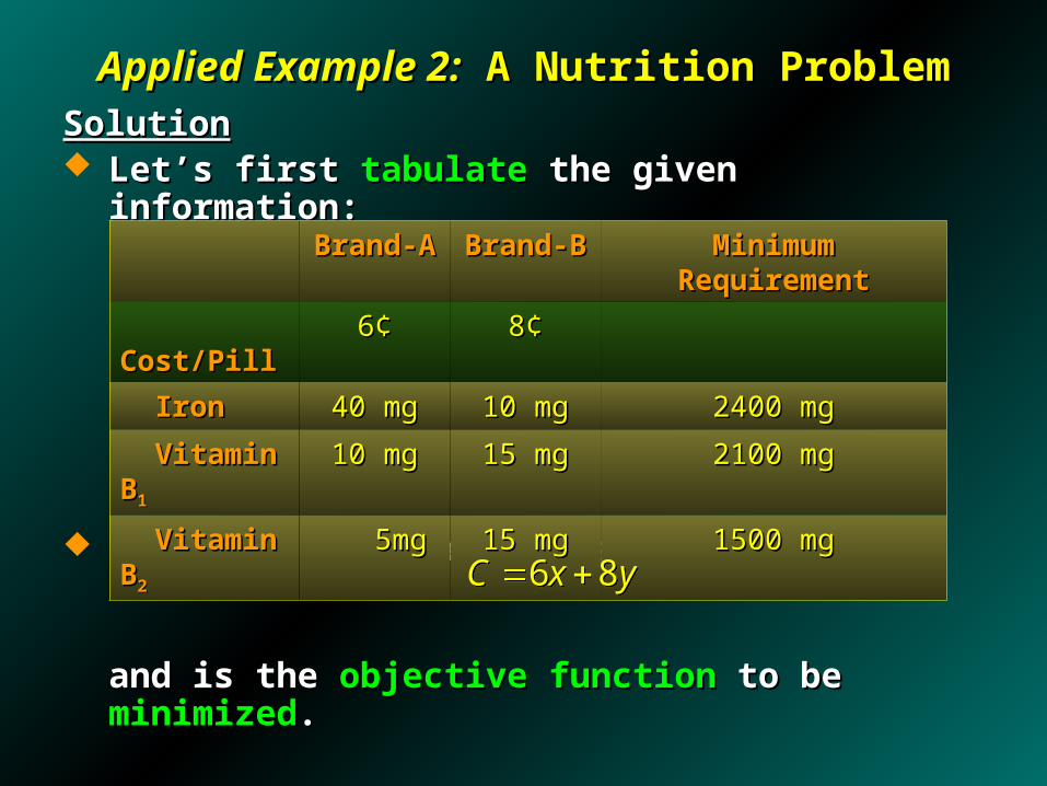
Applied Example 2:Applied Example 2: A Nutrition Problem A Nutrition ProblemSolutionSolution Let’s first Let’s first tabulatetabulate the given information: the given information:
The The costcost CC (in cents) is given by (in cents) is given by
and is the and is the objective functionobjective function to be to be minimizedminimized..
Brand-ABrand-A Brand-BBrand-B Minimum RequirementMinimum Requirement
Cost/PillCost/Pill 66¢¢ 88¢¢
IronIron 40 mg40 mg 10 mg10 mg 2400 mg2400 mg
Vitamin BVitamin B11 10 mg10 mg 15 mg15 mg 2100 mg2100 mg
Vitamin BVitamin B22 5mg5mg 15 mg15 mg 1500 mg1500 mg
6 8C x y 6 8C x y
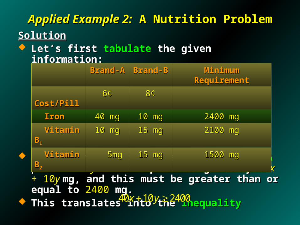
Applied Example 2:Applied Example 2: A Nutrition Problem A Nutrition ProblemSolutionSolution Let’s first Let’s first tabulatetabulate the given information: the given information:
The amount of The amount of ironiron contained in contained in x x brand-A brand-A pills and pills and yy brand-Bbrand-B pills is given by pills is given by 4040xx + 10 + 10y y mg, and this must be mg, and this must be greater than or equal to greater than or equal to 24002400 mg. mg.
This translates into the This translates into the inequalityinequality
Brand-ABrand-A Brand-BBrand-B Minimum RequirementMinimum Requirement
Cost/PillCost/Pill 66¢¢ 88¢¢
IronIron 40 mg40 mg 10 mg10 mg 2400 mg2400 mg
Vitamin BVitamin B11 10 mg10 mg 15 mg15 mg 2100 mg2100 mg
Vitamin BVitamin B22 5mg5mg 15 mg15 mg 1500 mg1500 mg
40 10 2400x y 40 10 2400x y

Applied Example 2:Applied Example 2: A Nutrition Problem A Nutrition ProblemSolutionSolution Let’s first Let’s first tabulatetabulate the given information: the given information:
The amount of The amount of vitamin Bvitamin B11 contained in contained in x x brand-A brand-A pills and pills and yy brand-Bbrand-B pills is given by pills is given by 1010xx + 15 + 15y y mg, and this must be mg, and this must be greater or equal to greater or equal to 21002100 mg. mg.
This translates into the This translates into the inequalityinequality
Brand-ABrand-A Brand-BBrand-B Minimum RequirementMinimum Requirement
Cost/PillCost/Pill 66¢¢ 88¢¢
IronIron 40 mg40 mg 10 mg10 mg 2400 mg2400 mg
Vitamin BVitamin B11 10 mg10 mg 15 mg15 mg 2100 mg2100 mg
Vitamin BVitamin B22 5mg5mg 15 mg15 mg 1500 mg1500 mg
10 15 2100x y 10 15 2100x y
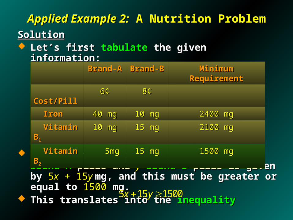
Applied Example 2:Applied Example 2: A Nutrition Problem A Nutrition ProblemSolutionSolution Let’s first Let’s first tabulatetabulate the given information: the given information:
The amount of The amount of vitamin Bvitamin B22 contained in contained in x x brand-A brand-A pills and pills and yy brand-Bbrand-B pills is given by pills is given by 55xx + 15 + 15y y mg, and this must be mg, and this must be greater or equal to greater or equal to 15001500 mg. mg.
This translates into the This translates into the inequalityinequality
Brand-ABrand-A Brand-BBrand-B Minimum RequirementMinimum Requirement
Cost/PillCost/Pill 66¢¢ 88¢¢
IronIron 40 mg40 mg 10 mg10 mg 2400 mg2400 mg
Vitamin BVitamin B11 10 mg10 mg 15 mg15 mg 2100 mg2100 mg
Vitamin BVitamin B22 5mg5mg 15 mg15 mg 1500 mg1500 mg
5 15 1500x y 5 15 1500x y

Applied Example 2:Applied Example 2: A Nutrition Problem A Nutrition ProblemSolutionSolution In short, we want to In short, we want to minimizeminimize the the objective functionobjective function
subject tosubject to the the system of inequalitiessystem of inequalities
We will discuss the We will discuss the solutionsolution to this problem in to this problem in section 6.4section 6.4..
5 15 1500x y 5 15 1500x y
6 8C x y 6 8C x y
40 10 2400x y 40 10 2400x y
10 15 2100x y 10 15 2100x y
0
0
x
y
0
0
x
y

6.36.3Graphical Solutions Graphical Solutions of Linear Programming Problemsof Linear Programming Problems
200200
100100
100100 200200 300300xx
yy
SS10 15 2100x y 10 15 2100x y
40 10 2400x y 40 10 2400x y
5 15 1500x y 5 15 1500x y
CC(120, 60)(120, 60)
DD(300, 0)(300, 0)
AA(0, 240)(0, 240)
BB(30, 120)(30, 120)
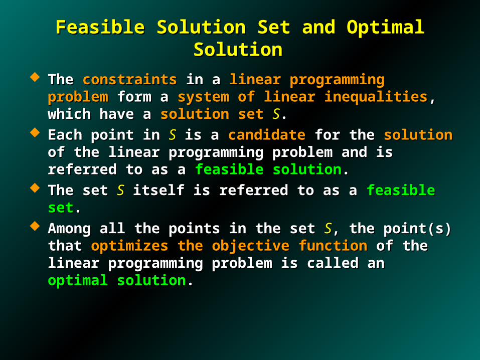
Feasible Solution Set and Optimal SolutionFeasible Solution Set and Optimal Solution
The The constraintsconstraints in a in a linear programming problemlinear programming problem form a form a system of linear inequalitiessystem of linear inequalities, which have a , which have a solution setsolution set SS..
Each point in Each point in SS is a is a candidatecandidate for the for the solutionsolution of the linear of the linear programming problem and is referred to as a programming problem and is referred to as a feasible feasible solutionsolution..
The set The set SS itself is referred to as a itself is referred to as a feasible setfeasible set.. Among all the points in the set Among all the points in the set SS, the point(s) that , the point(s) that
optimizes the objective functionoptimizes the objective function of the linear programming of the linear programming problem is called an problem is called an optimal solutionoptimal solution..

Theorem 1Theorem 1
Linear ProgrammingLinear Programming If a linear programming problem has a If a linear programming problem has a solutionsolution, ,
then it must occur at a then it must occur at a vertexvertex, or , or corner pointcorner point, , of the of the feasible setfeasible set SS associated with the problem. associated with the problem.
If the If the objective functionobjective function PP is is optimizedoptimized at at twotwo adjacent verticesadjacent vertices of of SS, then it is optimized , then it is optimized at at every every pointpoint on the line segment on the line segment joining these vertices, in joining these vertices, in which case there are which case there are infinitely many solutionsinfinitely many solutions to to the problem.the problem.

Theorem 2Theorem 2
Existence of a SolutionExistence of a Solution Suppose we are given a linear programming Suppose we are given a linear programming
problem with a problem with a feasible setfeasible set SS and an and an objective objective functionfunction PP = = axax + + byby..a.a. If If S S is is boundedbounded, then , then PP has both a has both a maximum and maximum and
a minimum value a minimum value on on SS..
b.b. If If S S is is unboundedunbounded and both and both aa and and bb are are nonnegativenonnegative, then , then PP has a has a minimum valueminimum value on on SS provided that the constraints definingprovided that the constraints defining S S include include the inequalities the inequalities xx 0 0 and and yy 0 0..
c.c. If If SS is the is the empty setempty set, then the linear , then the linear programming problem has programming problem has no solutionno solution: that is, : that is, PP has has neither a maximum nor a minimumneither a maximum nor a minimum value. value.
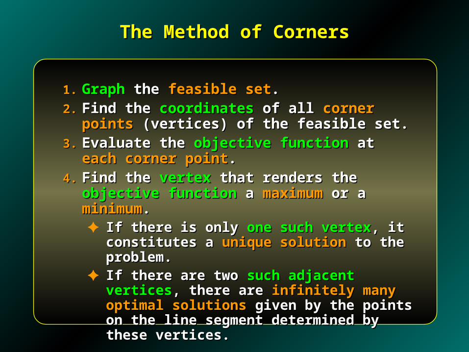
The Method of CornersThe Method of Corners
1.1. GraphGraph the the feasible setfeasible set..2.2. Find the Find the coordinatescoordinates of all of all corner pointscorner points
(vertices) of the feasible set.(vertices) of the feasible set.3.3. Evaluate the Evaluate the objective functionobjective function at at each corner each corner
pointpoint..4.4. Find the Find the vertexvertex that renders the that renders the objective objective
functionfunction a a maximummaximum or a or a minimumminimum..✦ If there is only If there is only one such vertexone such vertex, it constitutes a , it constitutes a
unique solutionunique solution to the problem. to the problem.✦ If there are two If there are two such adjacent verticessuch adjacent vertices, there , there
are are infinitely many optimal solutionsinfinitely many optimal solutions given by given by the points on the line segment determined by the points on the line segment determined by these vertices.these vertices.
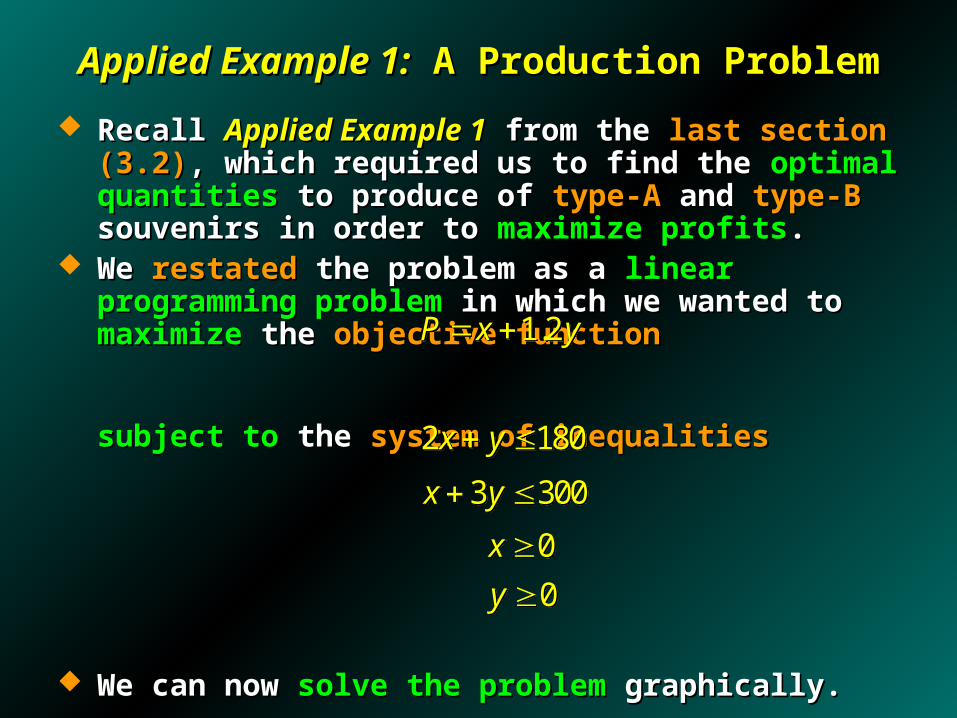
Applied Example 1:Applied Example 1: A Production Problem A Production Problem
Recall Recall Applied Example 1Applied Example 1 from the from the last section (3.2) last section (3.2), which , which required us to find the required us to find the optimal quantitiesoptimal quantities to produce of to produce of type-A type-A and and type-Btype-B souvenirs in order to souvenirs in order to maximize profitsmaximize profits..
We We restatedrestated the problem as a the problem as a linear programming problemlinear programming problem in which we wanted to in which we wanted to maximizemaximize the the objective functionobjective function
subject tosubject to the the system of inequalitiessystem of inequalities
We can now We can now solve the problemsolve the problem graphically. graphically.
0
0
x
y
0
0
x
y
1.2P x y 1.2P x y
3 300x y 3 300x y
2 180x y 2 180x y

200200
100100
100100 200200 300300
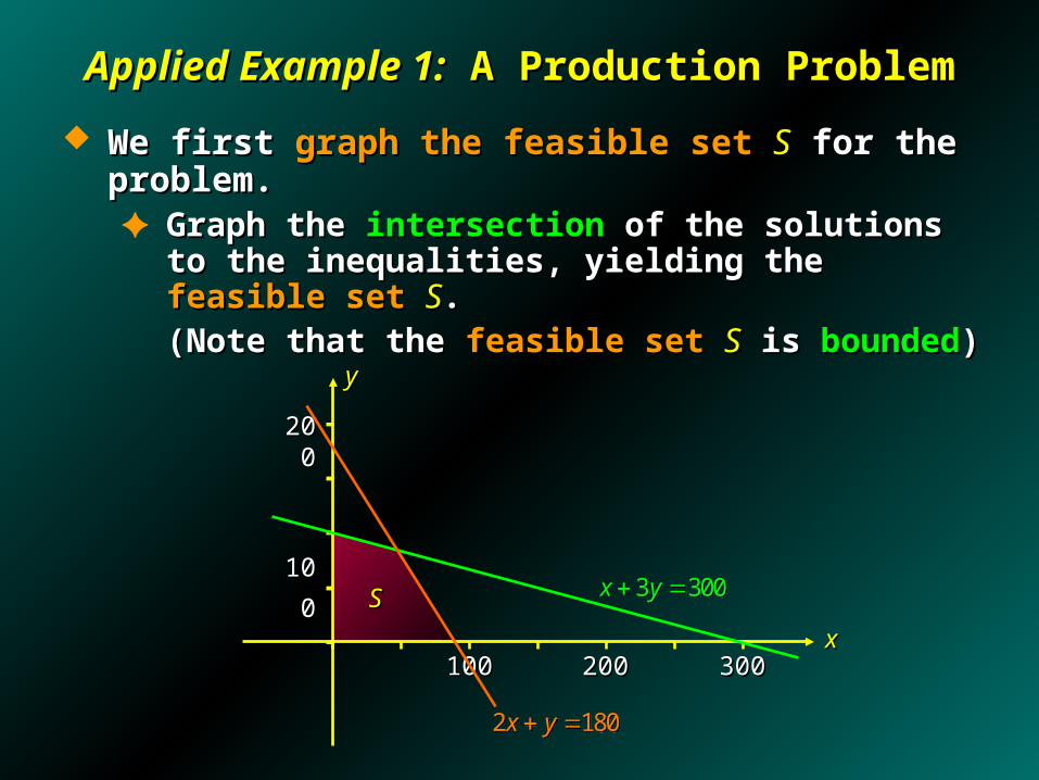
Applied Example 1:Applied Example 1: A Production Problem A Production Problem
We first We first graph the feasible setgraph the feasible set SS for the problem. for the problem.✦ Graph the Graph the solutionsolution for the inequality for the inequality
considering only considering only positive valuespositive values for for xx and and yy::
2 180x y 2 180x y
xx
yy
2 180x y 2 180x y
(90, 0)(90, 0)
(0, 180)(0, 180)
2 180x y 2 180x y

200200
100100
Applied Example 1:Applied Example 1: A Production Problem A Production Problem
We first We first graph the feasible setgraph the feasible set SS for the problem. for the problem.✦ Graph the Graph the solutionsolution for the inequality for the inequality
considering only considering only positive valuespositive values for for xx and and yy::
3 300x y 3 300x y
100100 200200 300300xx
yy
3 300x y 3 300x y
(0, 100)(0, 100)
(300, 0)(300, 0)
3 300x y 3 300x y
200200
100100
Applied Example 1:Applied Example 1: A Production Problem A Production Problem
We first We first graph the feasible setgraph the feasible set SS for the problem. for the problem.✦ Graph the Graph the intersectionintersection of the solutions to the inequalities, of the solutions to the inequalities,
yielding the yielding the feasible setfeasible set SS..(Note that the (Note that the feasible setfeasible set SS is is boundedbounded))
100100 200200 300300xx
yy
SS 3 300x y 3 300x y
2 180x y 2 180x y
200200
100100
Applied Example 1:Applied Example 1: A Production Problem A Production Problem
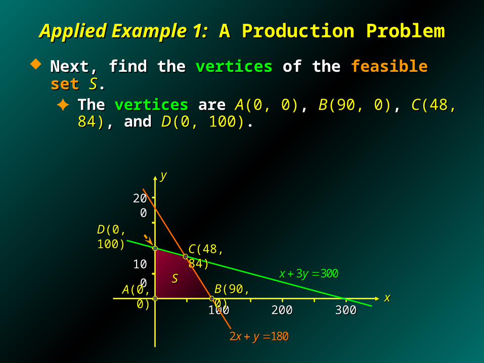
Next, find the Next, find the verticesvertices of the of the feasible setfeasible set SS. . ✦ The The verticesvertices are are AA(0, 0)(0, 0), , BB(90, 0)(90, 0), , CC(48, 84)(48, 84), and , and DD(0, 100)(0, 100)..
100100 200200 300300xx
yy
SS
CC(48, 84)(48, 84)
3 300x y 3 300x y
2 180x y 2 180x y
DD(0, 100)(0, 100)
BB(90, 0)(90, 0)AA(0, 0)(0, 0)
200200
100100
Applied Example 1:Applied Example 1: A Production Problem A Production Problem
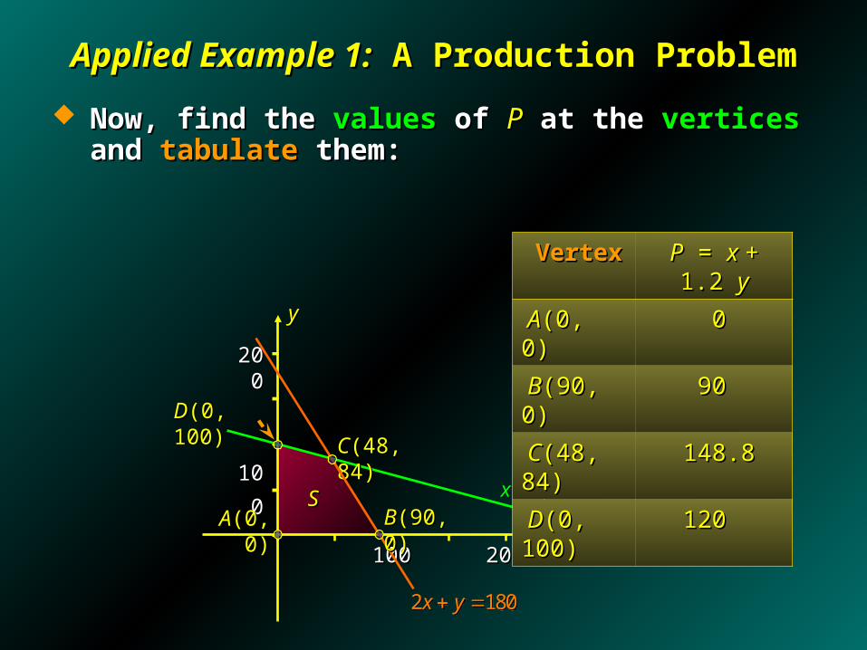
Now, find the Now, find the valuesvalues of of PP at the at the verticesvertices and and tabulate tabulate them:them:
100100 200200 300300xx
yy
SS
CC(48, 84)(48, 84)
3 300x y 3 300x y
2 180x y 2 180x y
DD(0, 100)(0, 100)
BB(90, 0)(90, 0)AA(0, 0)(0, 0)
VertexVertex PP = = x x + 1.2 + 1.2 yy
AA(0, 0)(0, 0) 00
BB(90, 0)(90, 0) 9090
CC(48, 84)(48, 84) 148.8148.8
DD(0, 100)(0, 100) 120120

200200
100100
Applied Example 1:Applied Example 1: A Production Problem A Production Problem
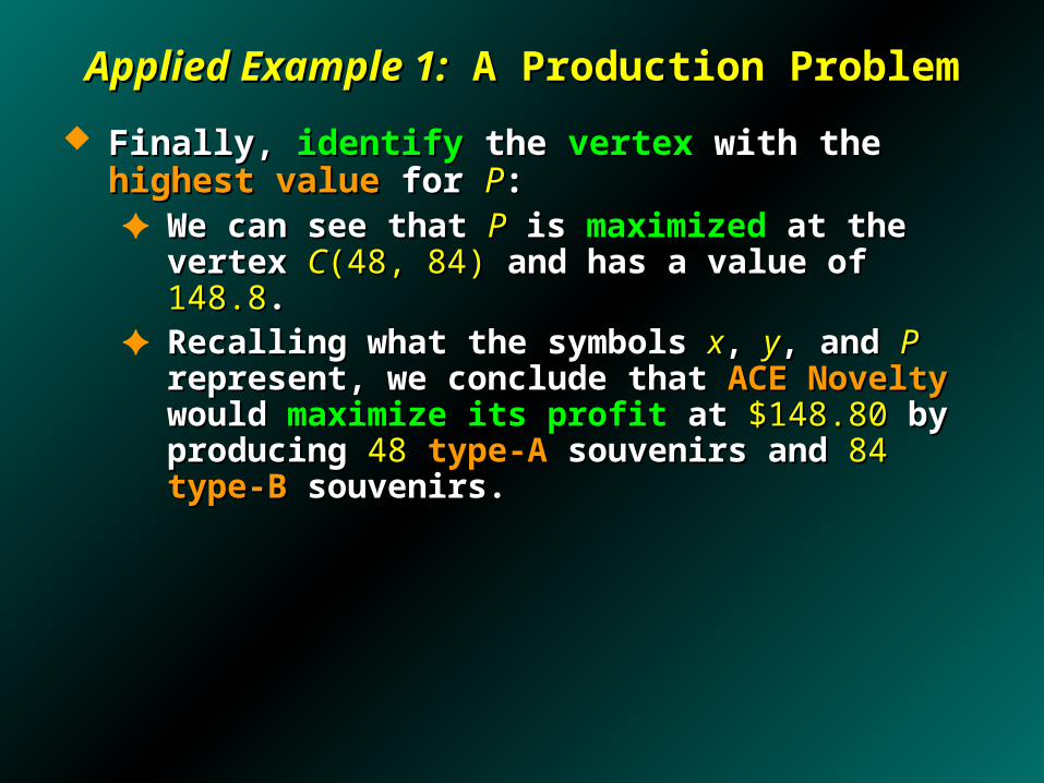
Finally, Finally, identifyidentify the the vertexvertex with the with the highest valuehighest value for for PP::✦ We can see that We can see that PP is is maximizedmaximized at the vertex at the vertex CC(48, 84)(48, 84)
and has a value of and has a value of 148.8148.8..
100100 200200 300300xx
yy
SS 3 300x y 3 300x y
2 180x y 2 180x y
DD(0, 100)(0, 100)
BB(90, 0)(90, 0)AA(0, 0)(0, 0)
VertexVertex PP = = x x + 1.2 + 1.2 yy
AA(0, 0)(0, 0) 00
BB(90, 0)(90, 0) 9090
CC(48, 84)(48, 84) 148.8148.8
DD(0, 100)(0, 100) 120120
CC(48, 84)(48, 84)
Applied Example 1:Applied Example 1: A Production Problem A Production Problem
Finally, Finally, identifyidentify the the vertexvertex with the with the highest valuehighest value for for PP::✦ We can see that We can see that PP is is maximizedmaximized at the vertex at the vertex CC(48, 84)(48, 84)
and has a value of and has a value of 148.8148.8..✦ Recalling what the symbols Recalling what the symbols xx, , yy, and , and PP represent, we represent, we
conclude that conclude that ACE NoveltyACE Novelty would would maximize its profitmaximize its profit at at $148.80$148.80 by producing by producing 4848 type-A type-A souvenirs and souvenirs and 8484 type-Btype-B souvenirs.souvenirs.
Applied Example 2:Applied Example 2: A Nutrition Problem A Nutrition Problem
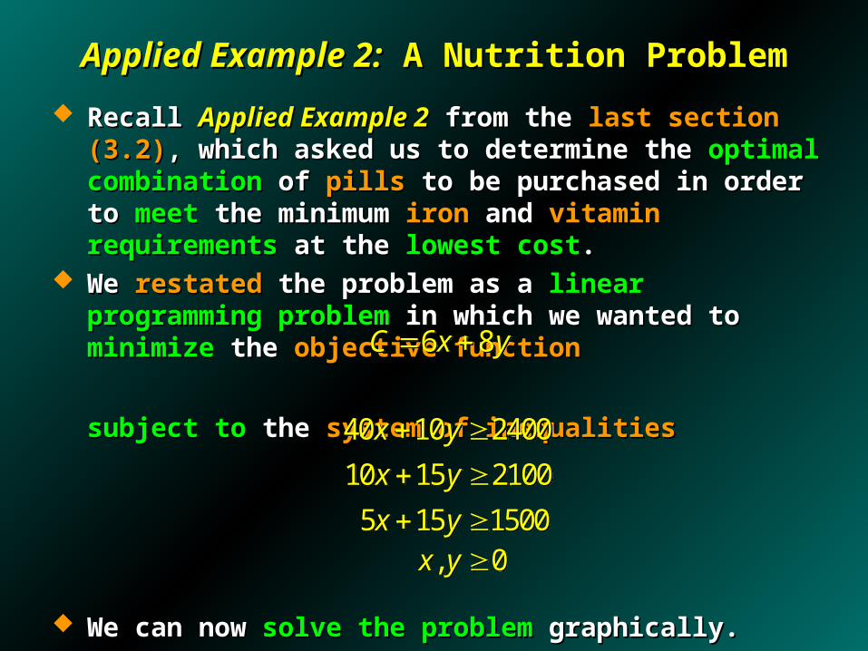
Recall Recall Applied Example 2Applied Example 2 from the from the last section (3.2) last section (3.2), which , which asked us to determine the asked us to determine the optimal combinationoptimal combination ofof pills pills to to be purchased in order to be purchased in order to meetmeet the minimum the minimum ironiron and and vitaminvitamin requirementsrequirements at the at the lowest costlowest cost..
We We restatedrestated the problem as a the problem as a linear programming problemlinear programming problem in which we wanted to in which we wanted to minimizeminimize the the objective functionobjective function
subject tosubject to the the system of inequalitiessystem of inequalities
We can now We can now solve the problemsolve the problem graphically. graphically.
5 15 1500x y 5 15 1500x y
6 8C x y 6 8C x y
40 10 2400x y 40 10 2400x y
10 15 2100x y 10 15 2100x y
, 0x y , 0x y
200200
100100
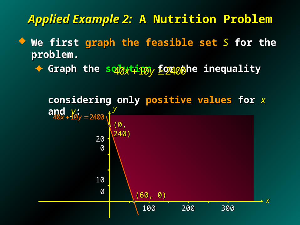
Applied Example 2:Applied Example 2: A Nutrition Problem A Nutrition Problem
We first We first graph the feasible setgraph the feasible set SS for the problem. for the problem.✦ Graph the Graph the solutionsolution for the inequality for the inequality
considering only considering only positive valuespositive values for for xx and and yy::
100100 200200 300300xx
yy40 10 2400x y 40 10 2400x y
40 10 2400x y 40 10 2400x y
(60, 0)(60, 0)
(0, 240)(0, 240)

200200
100100
Applied Example 2:Applied Example 2: A Nutrition Problem A Nutrition Problem
We first We first graph the feasible setgraph the feasible set SS for the problem. for the problem.✦ Graph the Graph the solutionsolution for the inequality for the inequality
considering only considering only positive valuespositive values for for xx and and yy::
100100 200200 300300xx
yy
10 15 2100x y 10 15 2100x y
10 15 2100x y 10 15 2100x y
(210, 0)(210, 0)
(0, 140)(0, 140)

200200
100100
Applied Example 2:Applied Example 2: A Nutrition Problem A Nutrition Problem
We first We first graph the feasible setgraph the feasible set SS for the problem. for the problem.✦ Graph the Graph the solutionsolution for the inequality for the inequality
considering only considering only positive valuespositive values for for xx and and yy::
100100 200200 300300xx
yy
5 15 1500x y 5 15 1500x y
5 15 1500x y 5 15 1500x y
(300, 0)(300, 0)
(0, 100)(0, 100)

200200
100100
Applied Example 2:Applied Example 2: A Nutrition Problem A Nutrition Problem
We first We first graph the feasible setgraph the feasible set SS for the problem. for the problem.✦ Graph the Graph the intersectionintersection of the solutions to the inequalities, of the solutions to the inequalities,
yielding the yielding the feasible setfeasible set SS..
(Note that the (Note that the feasible setfeasible set SS is is unboundedunbounded))
100100 200200 300300xx
yy
SS10 15 2100x y 10 15 2100x y
40 10 2400x y 40 10 2400x y
5 15 1500x y 5 15 1500x y
200200
100100
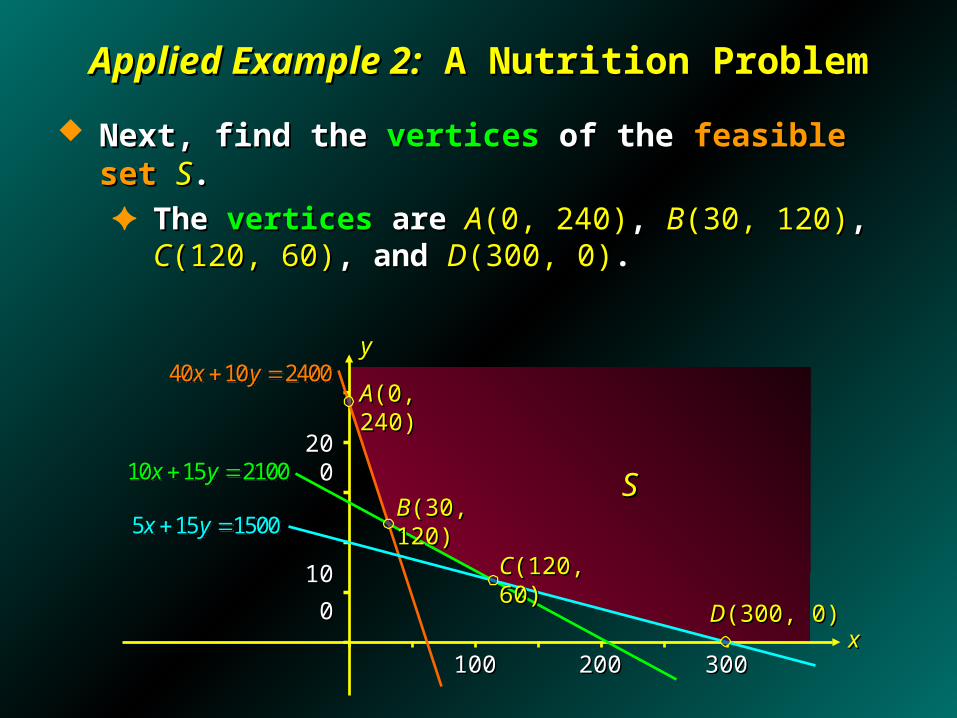
Applied Example 2:Applied Example 2: A Nutrition Problem A Nutrition Problem
Next, find the Next, find the verticesvertices of the of the feasible setfeasible set SS. . ✦ The The verticesvertices are are AA(0, 240)(0, 240), , BB(30, 120)(30, 120), , CC(120, 60)(120, 60), and , and
DD(300, 0)(300, 0)..
100100 200200 300300xx
yy
SS10 15 2100x y 10 15 2100x y
40 10 2400x y 40 10 2400x y
5 15 1500x y 5 15 1500x y
CC(120, 60)(120, 60)
DD(300, 0)(300, 0)
AA(0, 240)(0, 240)
BB(30, 120)(30, 120)

Applied Example 2:Applied Example 2: A Nutrition Problem A Nutrition Problem
Now, find the Now, find the valuesvalues of of CC at the at the verticesvertices and and tabulate tabulate them:them:
200200
100100
100100 200200 300300xx
yy
SS10 15 2100x y 10 15 2100x y
40 10 2400x y 40 10 2400x y
5 15 1500x y 5 15 1500x y
CC(120, 60)(120, 60)
DD(300, 0)(300, 0)
AA(0, 240)(0, 240)
BB(30, 120)(30, 120)
VertexVertex CC = 6 = 6x x + 8+ 8yy
AA(0, 240)(0, 240) 19201920
BB(30, 120)(30, 120) 11401140
CC(120, 60)(120, 60) 12001200
DD(300, 0)(300, 0) 18001800

Applied Example 2:Applied Example 2: A Nutrition Problem A Nutrition Problem
Finally, Finally, identifyidentify the the vertexvertex with the with the lowest valuelowest value for for CC::✦ We can see that We can see that CC is is minimizedminimized at the vertex at the vertex BB(30, 120)(30, 120)
and has a value of and has a value of 11401140..
200200
100100
100100 200200 300300xx
yy
SS10 15 2100x y 10 15 2100x y
40 10 2400x y 40 10 2400x y
5 15 1500x y 5 15 1500x y
CC(120, 60)(120, 60)
DD(300, 0)(300, 0)
AA(0, 240)(0, 240)
VertexVertex CC = 6 = 6x x + 8+ 8yy
AA(0, 240)(0, 240) 19201920
BB(30, 120)(30, 120) 11401140
CC(120, 60)(120, 60) 12001200
DD(300, 0)(300, 0) 18001800
BB(30, 120)(30, 120)

Applied Example 2:Applied Example 2: A Nutrition Problem A Nutrition Problem
Finally, Finally, identifyidentify the the vertexvertex with the with the lowest valuelowest value for for CC::✦ We can see that We can see that CC is is minimizedminimized at the vertex at the vertex BB(30, 120)(30, 120)
and has a value of and has a value of 11401140..✦ Recalling what the symbols Recalling what the symbols xx, , yy, and , and CC represent, we represent, we
conclude that the individual should conclude that the individual should purchasepurchase 3030 brand-A brand-A pills and pills and 120120 brand-Bbrand-B pills at a pills at a minimum costminimum cost of of $11.40$11.40..

6.46.4The Simplex Method: The Simplex Method: Standard Maximization ProblemsStandard Maximization Problems
xx yy uu vv PP ConstantConstant
11 00 3/53/5 ––1/51/5 00 4848
00 1 1 ––1/51/5 2/52/5 00 8484
0 0 00 9/259/25 7/257/25 11 148148 4/54/5
The Simplex MethodThe Simplex Method
The The simplex methodsimplex method is an is an iterative procedureiterative procedure.. Beginning at a Beginning at a vertexvertex of the of the feasible regionfeasible region SS, each , each
iterationiteration brings us to another brings us to another vertexvertex of of SS with an with an improvedimproved value of the value of the objective functionobjective function..
The The iterationiteration ends when the ends when the optimal solutionoptimal solution is reached. is reached.

A Standard Linear Programming ProblemA Standard Linear Programming Problem
A A standard maximization problemstandard maximization problem is one in which is one in which
1.1. The The objective functionobjective function is to be is to be maximizedmaximized..
2.2. All the All the variablesvariables involved in the problem are involved in the problem are nonnegativenonnegative..
3.3. All other All other linear constraintslinear constraints may be written so may be written so that the expression involving the variables is that the expression involving the variables is less less than or equal tothan or equal to a nonnegative constanta nonnegative constant..

Setting Up the Initial Simplex TableauSetting Up the Initial Simplex Tableau
1.1. Transform the Transform the system of linearsystem of linear inequalitiesinequalities into a into a system of linearsystem of linear equationsequations by by introducing introducing slack variablesslack variables..
2.2. Rewrite the Rewrite the objective functionobjective function
in the formin the form
where all the where all the variablesvariables are on the are on the leftleft and the and the coefficientcoefficient of of PP is is +1+1. Write this equation . Write this equation below the equations in below the equations in step 1step 1..
3.3. Write the Write the augmented matrixaugmented matrix associated with associated with this system of linear equations.this system of linear equations.
1 1 2 2 n nP c x c x c x 1 1 2 2 n nP c x c x c x
1 1 2 2 0n nc x c x c x P 1 1 2 2 0n nc x c x c x P
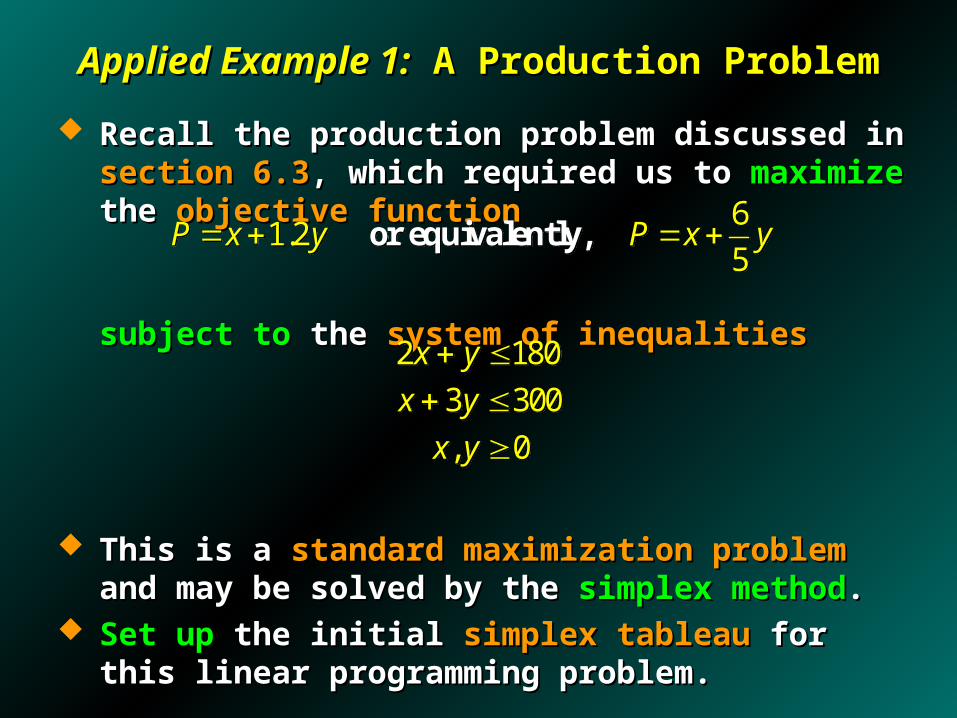
Applied Example 1:Applied Example 1: A Production Problem A Production Problem
Recall the production problem discussed in Recall the production problem discussed in section 6.3section 6.3, , which required us to which required us to maximizemaximize the the objective functionobjective function
subject tosubject to the the system of inequalitiessystem of inequalities
This is a This is a standard maximization problemstandard maximization problem and may be and may be solved by the solved by the simplex methodsimplex method..
Set upSet up the initial the initial simplex tableausimplex tableau for this linear for this linear programming problem.programming problem.
, 0x y , 0x y
61.2
5P x y P x y or equivalently,
61.2
5P x y P x y or equivalently,
3 300x y 3 300x y 2 180x y 2 180x y

Applied Example 1:Applied Example 1: A Production Problem A Production ProblemSolutionSolution First, introduce the First, introduce the slack variablesslack variables uu and and vv into the into the
inequalities inequalities
and turn these into and turn these into equationsequations, getting, getting
Next, rewrite the Next, rewrite the objective functionobjective function in the form in the form
2 180
3 300
x y u
x y v
2 180
3 300
x y u
x y v
3 300x y 3 300x y
2 180x y 2 180x y
60
5x y P
60
5x y P

Applied Example 1:Applied Example 1: A Production Problem A Production ProblemSolutionSolution Placing the restated Placing the restated objective functionobjective function below the system of below the system of
equations of the equations of the constraintsconstraints we get we get
Thus, the Thus, the initial tableauinitial tableau associated with this system is associated with this system is
2 180
3 300
60
5
x y u
x y v
x y P
2 180
3 300
60
5
x y u
x y v
x y P
xx yy uu vv PP ConstantConstant
22 11 11 00 00 180180
11 3 3 00 11 00 300300
––1 1 –– 6/56/5 00 00 11 00

The Simplex MethodThe Simplex Method
1.1. Set up the Set up the initial simplex tableauinitial simplex tableau..2.2. Determine whether the Determine whether the optimal solutionoptimal solution has has
been reached by been reached by examining all entriesexamining all entries in the in the last last rowrow to the to the leftleft of the of the vertical linevertical line..a.a. If all the entries are If all the entries are nonnegativenonnegative, the , the optimal optimal
solutionsolution hashas been reached been reached. Proceed to . Proceed to step 4step 4..b.b. If there are one or more If there are one or more negative entriesnegative entries, the , the
optimal solutionoptimal solution has nothas not been reached been reached. . Proceed to Proceed to step 3step 3..
3.3. Perform the Perform the pivot operationpivot operation. Return to . Return to step 2step 2..4.4. Determine the Determine the optimal solution(s)optimal solution(s)..
Applied Example 1:Applied Example 1: A Production Problem A Production Problem
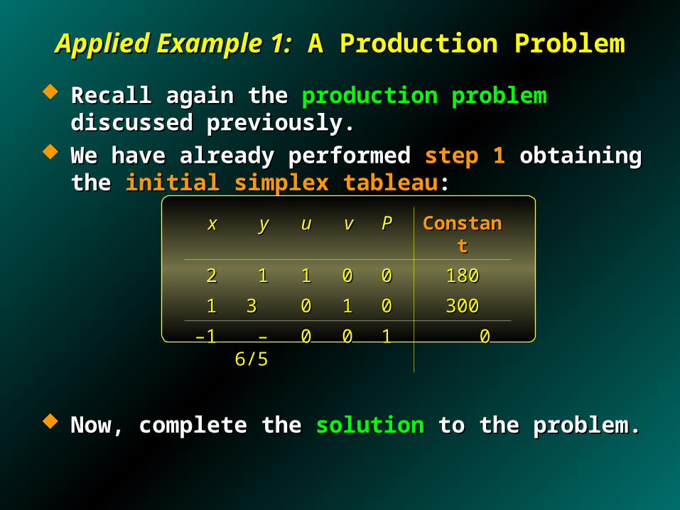
Recall again the Recall again the production problemproduction problem discussed previously. discussed previously. We have already performed We have already performed step 1step 1 obtaining the obtaining the initial initial
simplex tableausimplex tableau::
Now, complete the Now, complete the solutionsolution to the problem. to the problem.
xx yy uu vv PP ConstantConstant
22 11 11 00 00 180180
11 3 3 00 11 00 300300
––1 1 –– 6/56/5 00 00 11 00

Applied Example 1:Applied Example 1: A Production Problem A Production ProblemSolutionSolution
Step 2.Step 2. Determine whether the Determine whether the optimal solutionoptimal solution has been has been reached.reached.
✦ Since Since there there areare negative entries negative entries in the last row of the in the last row of the tableau, the tableau, the initial solutioninitial solution is is notnot optimal optimal..
xx yy uu vv PP ConstantConstant
22 11 11 00 00 180180
11 3 3 00 11 00 300300
––1 1 –– 6/56/5 00 00 11 00
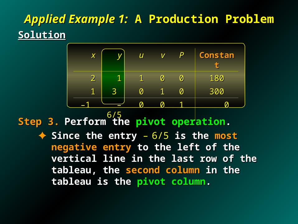
Applied Example 1:Applied Example 1: A Production Problem A Production ProblemSolutionSolution
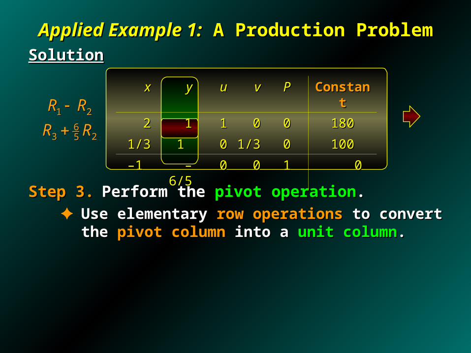
Step 3.Step 3. Perform the Perform the pivot operationpivot operation..✦ Since the entry Since the entry –– 6/56/5 isis the the most negative entrymost negative entry to the left to the left
of the vertical line in the last row of the tableau, the of the vertical line in the last row of the tableau, the second columnsecond column in the tableau is the in the tableau is the pivot columnpivot column..
xx yy uu vv PP ConstantConstant
22 11 11 00 00 180180
11 3 3 00 11 00 300300
––1 1 –– 6/56/5 00 00 11 00

Applied Example 1:Applied Example 1: A Production Problem A Production ProblemSolutionSolution
Step 3.Step 3. Perform the Perform the pivot operationpivot operation..✦ Divide each Divide each positive numberpositive number of the of the pivot columnpivot column into the into the
corresponding entrycorresponding entry in the in the column of constantscolumn of constants and and compare compare thethe ratiosratios thus obtained. thus obtained.
✦ We see that the We see that the ratioratio 300/3 = 100300/3 = 100 is is less thanless than the the ratioratio 180/1 = 180180/1 = 180, so , so row 2row 2 is the is the pivot rowpivot row..
xx yy uu vv PP ConstantConstant
22 11 11 00 00 180180
11 3 3 00 11 00 300300
––1 1 –– 6/56/5 00 00 11 00
1801
3003
180
100
1801
3003
180
100
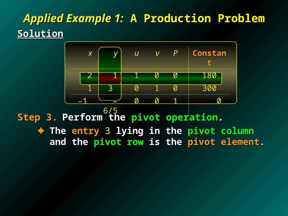
Applied Example 1:Applied Example 1: A Production Problem A Production ProblemSolutionSolution
Step 3.Step 3. Perform the Perform the pivot operationpivot operation..✦ The The entryentry 3 3 lying in the lying in the pivot columnpivot column and the and the pivot rowpivot row
is the is the pivot elementpivot element..
xx yy uu vv PP ConstantConstant
22 11 11 00 00 180180
11 3 3 00 11 00 300300
––1 1 –– 6/56/5 00 00 11 00
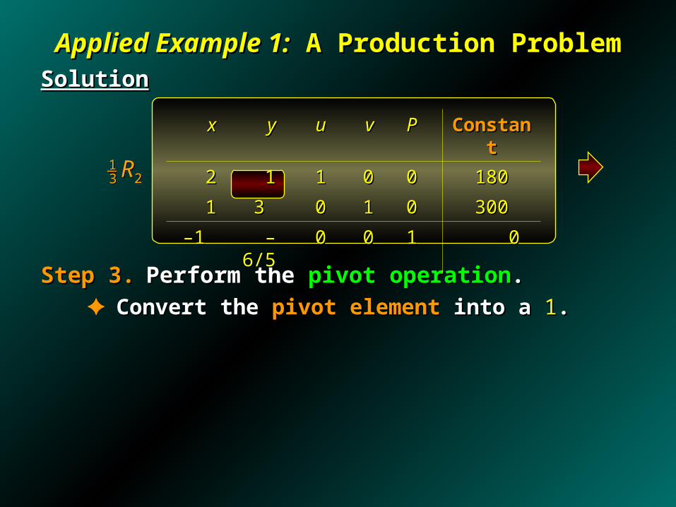
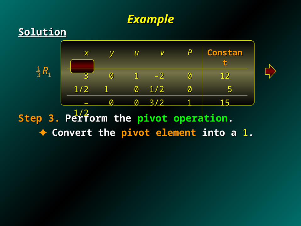
Applied Example 1:Applied Example 1: A Production Problem A Production ProblemSolutionSolution
Step 3.Step 3. Perform the Perform the pivot operationpivot operation..✦ Convert the Convert the pivot elementpivot element into a into a 1 1..
123 R123 R
xx yy uu vv PP ConstantConstant
22 11 11 00 00 180180
11 3 3 00 11 00 300300
––1 1 –– 6/56/5 00 00 11 00

Applied Example 1:Applied Example 1: A Production Problem A Production ProblemSolutionSolution
Step 3.Step 3. Perform the Perform the pivot operationpivot operation..✦ Convert the Convert the pivot elementpivot element into a into a 1 1..
123 R123 R
xx yy uu vv PP ConstantConstant
22 11 11 00 00 180180
1/31/3 1 1 00 1/31/3 00 100100
––1 1 –– 6/56/5 00 00 11 00
Applied Example 1:Applied Example 1: A Production Problem A Production ProblemSolutionSolution
Step 3.Step 3. Perform the Perform the pivot operationpivot operation..✦ Use elementary Use elementary row operationsrow operations to convert the to convert the pivot pivot
columncolumn into a into a unit columnunit column..
1 2
63 25
R R
R R
1 2
63 25
R R
R R
xx yy uu vv PP ConstantConstant
22 11 11 00 00 180180
1/31/3 1 1 00 1/31/3 00 100100
––1 1 –– 6/56/5 00 00 11 00

Applied Example 1:Applied Example 1: A Production Problem A Production ProblemSolutionSolution
Step 3.Step 3. Perform the Perform the pivot operationpivot operation..✦ Use elementary Use elementary row operationsrow operations to convert the to convert the pivot pivot
columncolumn into a into a unit columnunit column..
1 2
63 25
R R
R R
1 2
63 25
R R
R R
xx yy uu vv PP ConstantConstant
5/35/3 00 11 ––1/31/3 00 8080
1/31/3 1 1 00 1/31/3 00 100100
––3/5 3/5 00 00 2/52/5 11 120120

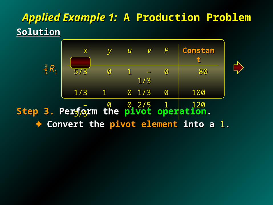
Applied Example 1:Applied Example 1: A Production Problem A Production ProblemSolutionSolution
Step 3.Step 3. Perform the Perform the pivot operationpivot operation..✦ This This completes an iterationcompletes an iteration..
✦ The The last rowlast row of the tableau contains a of the tableau contains a negative numbernegative number, , so an so an optimal solutionoptimal solution hashas notnot been reached been reached..
✦ Therefore, we Therefore, we repeatrepeat the the iteration stepiteration step..
xx yy uu vv PP ConstantConstant
5/35/3 00 11 ––1/31/3 00 8080
1/31/3 1 1 00 1/31/3 00 100100
––3/5 3/5 00 00 2/52/5 11 120120
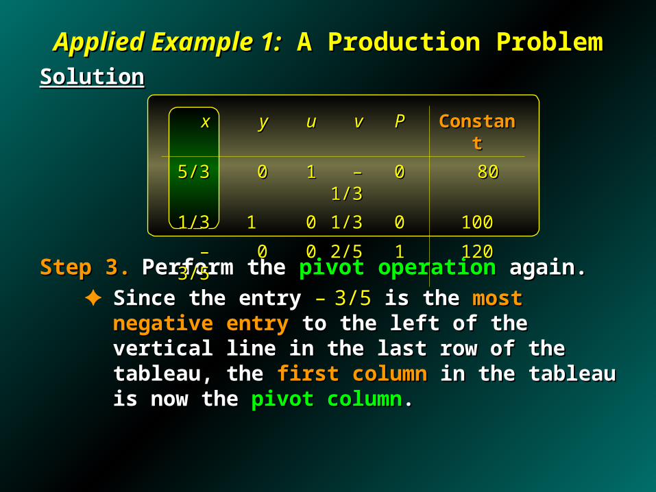
Applied Example 1:Applied Example 1: A Production Problem A Production ProblemSolutionSolution
Step 3.Step 3. Perform the Perform the pivot operationpivot operation again. again.✦ Since the entry Since the entry –– 3/53/5 isis the the most negative entrymost negative entry to the left to the left
of the vertical line in the last row of the tableau, the of the vertical line in the last row of the tableau, the first first columncolumn in the tableau is now the in the tableau is now the pivot columnpivot column..
xx yy uu vv PP ConstantConstant
5/35/3 00 11 ––1/31/3 00 8080
1/31/3 1 1 00 1/31/3 00 100100
––3/5 3/5 00 00 2/52/5 11 120120
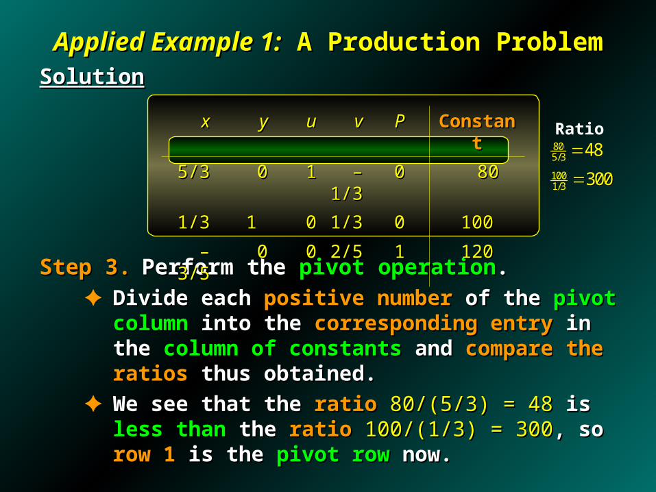
Applied Example 1:Applied Example 1: A Production Problem A Production ProblemSolutionSolution
Step 3.Step 3. Perform the Perform the pivot operationpivot operation..✦ Divide each Divide each positive numberpositive number of the of the pivot columnpivot column into the into the
corresponding entrycorresponding entry in the in the column of constantscolumn of constants and and compare the ratioscompare the ratios thus obtained. thus obtained.
✦ We see that the We see that the ratioratio 80/(5/3) = 4880/(5/3) = 48 is is less thanless than the the ratioratio 100/(1/3) = 300100/(1/3) = 300, so , so row 1row 1 is the is the pivot rowpivot row now. now.
xx yy uu vv PP ConstantConstant
5/35/3 00 11 ––1/31/3 00 8080
1/31/3 1 1 00 1/31/3 00 100100
––3/5 3/5 00 00 2/52/5 11 120120
805/3
1001/3
48
300
805/3
1001/3
48
300
Ratio
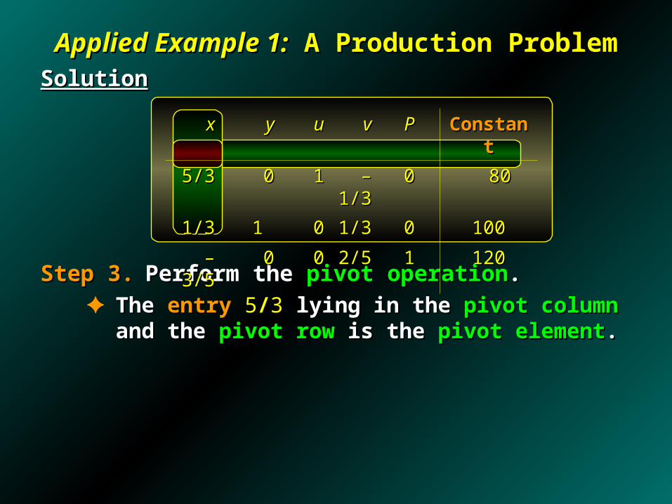
Applied Example 1:Applied Example 1: A Production Problem A Production ProblemSolutionSolution
Step 3.Step 3. Perform the Perform the pivot operationpivot operation..✦ The The entryentry 55//3 3 lying in the lying in the pivot columnpivot column and the and the pivot pivot
rowrow is the is the pivot elementpivot element..
xx yy uu vv PP ConstantConstant
5/35/3 00 11 ––1/31/3 00 8080
1/31/3 1 1 00 1/31/3 00 100100
––3/5 3/5 00 00 2/52/5 11 120120
Applied Example 1:Applied Example 1: A Production Problem A Production ProblemSolutionSolution
Step 3.Step 3. Perform the Perform the pivot operationpivot operation..✦ Convert the Convert the pivot elementpivot element into a into a 1 1..
xx yy uu vv PP ConstantConstant
5/35/3 00 11 ––1/31/3 00 8080
1/31/3 1 1 00 1/31/3 00 100100
––3/5 3/5 00 00 2/52/5 11 120120
315 R315 R
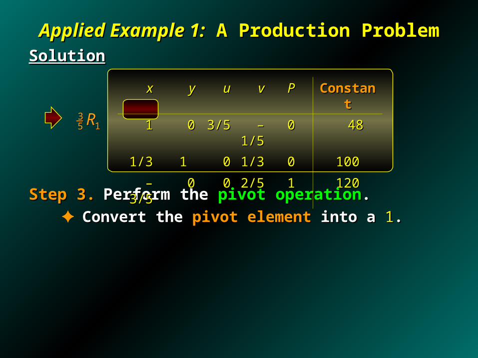
Applied Example 1:Applied Example 1: A Production Problem A Production ProblemSolutionSolution
Step 3.Step 3. Perform the Perform the pivot operationpivot operation..✦ Convert the Convert the pivot elementpivot element into a into a 1 1..
xx yy uu vv PP ConstantConstant
11 00 3/53/5 ––1/51/5 00 4848
1/31/3 1 1 00 1/31/3 00 100100
––3/5 3/5 00 00 2/52/5 11 120120
315 R315 R
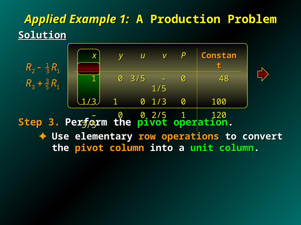
Applied Example 1:Applied Example 1: A Production Problem A Production ProblemSolutionSolution
Step 3.Step 3. Perform the Perform the pivot operationpivot operation..✦ Use elementary Use elementary row operationsrow operations to convert the to convert the pivot pivot
columncolumn into a into a unit columnunit column..
12 13
33 15
R R
R R
12 13
33 15
R R
R R
xx yy uu vv PP ConstantConstant
11 00 3/53/5 ––1/51/5 00 4848
1/31/3 1 1 00 1/31/3 00 100100
––3/5 3/5 00 00 2/52/5 11 120120

Applied Example 1:Applied Example 1: A Production Problem A Production ProblemSolutionSolution
Step 3.Step 3. Perform the Perform the pivot operationpivot operation..✦ Use elementary Use elementary row operationsrow operations to convert the to convert the pivot pivot
columncolumn into a into a unit columnunit column..
12 13
33 15
R R
R R
12 13
33 15
R R
R R
xx yy uu vv PP ConstantConstant
11 00 3/53/5 ––1/51/5 00 4848
00 1 1 ––1/51/5 2/52/5 00 8484
0 0 00 9/259/25 7/257/25 11 148148 4/54/5

Applied Example 1:Applied Example 1: A Production Problem A Production ProblemSolutionSolution
Step 3.Step 3. Perform the Perform the pivot operationpivot operation..✦ The The last rowlast row of the tableau contains of the tableau contains nono negative negative
numbersnumbers, so an , so an optimal solutionoptimal solution hashas been reached been reached..
xx yy uu vv PP ConstantConstant
11 00 3/53/5 ––1/51/5 00 4848
00 1 1 ––1/51/5 2/52/5 00 8484
0 0 00 9/259/25 7/257/25 11 148148 4/54/5

Applied Example 1:Applied Example 1: A Production Problem A Production ProblemSolutionSolution
Step 4.Step 4. Determine the Determine the optimal solutionoptimal solution..✦ Locate the Locate the basic variablesbasic variables in the final tableau. in the final tableau.
In this case, the In this case, the basic variablesbasic variables are are xx, , yy, and , and PP.. The The optimal valueoptimal value for for xx is is 4848.. The The optimal valueoptimal value for for yy is is 8484.. The The optimal valueoptimal value for for PP is is 148.8148.8..
✦ Thus, the firm will Thus, the firm will maximize profitsmaximize profits at at $148.80$148.80 by by producing producing 4848 type-A type-A souvenirs and souvenirs and 84 84 type-Btype-B souvenirs. souvenirs.This This agreesagrees with the results obtained in with the results obtained in section 6.3section 6.3..
xx yy uu vv PP ConstantConstant
11 00 3/53/5 ––1/51/5 00 4848
00 1 1 ––1/51/5 2/52/5 00 8484
0 0 00 9/259/25 7/257/25 11 148148 4/54/5

6.56.5The Simplex Method: The Simplex Method: Standard Minimization ProblemsStandard Minimization Problems
3030
––1/501/50
3/1003/100
xx
00
11
00
vv
450450
11/1011/10
––3/203/20
ww
0 0
00
11
uu
1140114011120120
13/2513/25002/252/25
1/501/5000––1/501/50
ConstantConstantPPyy
3030
––1/501/50
3/1003/100
xx
00
11
00
vv
450450
11/1011/10
––3/203/20
ww
0 0
00
11
uu
1140114011120120
13/2513/25002/252/25
1/501/5000––1/501/50
ConstantConstantPPyy
SolutionSolution for thefor theprimal problemprimal problem
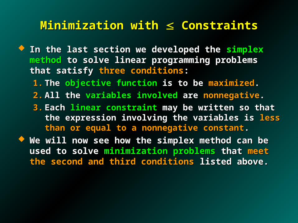
Minimization with Minimization with Constraints Constraints
In the last section we developed the In the last section we developed the simplex methodsimplex method to to solve linear programming problems that satisfy solve linear programming problems that satisfy three three conditionsconditions::
1.1. The The objective functionobjective function is to be is to be maximizedmaximized..
2.2. All the All the variables involvedvariables involved are are nonnegativenonnegative..
3.3. Each Each linear constraintlinear constraint may be written so that the may be written so that the expression involving the variables is expression involving the variables is less than or equal to less than or equal to a nonnegative constanta nonnegative constant..
We will now see how the simplex method can be used to We will now see how the simplex method can be used to solve solve minimization problemsminimization problems that that meet the second and meet the second and third conditionsthird conditions listed above. listed above.

ExampleExample
Solve the following Solve the following linear programming problemlinear programming problem::
This problem involves the This problem involves the minimizationminimization of the objective of the objective function and so is function and so is notnot a a standard maximization problemstandard maximization problem..
Note, however, that Note, however, that all the other conditionsall the other conditions for a for a standard standard maximizationmaximization hold truehold true..
2 3Minimize C x y 2 3Minimize C x y
5 4 32
2 10
, 0
subject to x y
x y
x y
5 4 32
2 10
, 0
subject to x y
x y
x y

ExampleExample
We can use the We can use the simplex methodsimplex method to solve this problem by to solve this problem by convertingconverting the the objective functionobjective function from from minimizingminimizing CC to its to its equivalentequivalent of of maximizingmaximizing PP = –= – CC. .
Thus, the Thus, the restatedrestated linear programming problemlinear programming problem is is
This problem can now be solved using the This problem can now be solved using the simplex methodsimplex method as discussed in as discussed in section 6.4section 6.4..
2 3Maximize P x y 2 3Maximize P x y
5 4 32
2 10
, 0
subject to x y
x y
x y
5 4 32
2 10
, 0
subject to x y
x y
x y
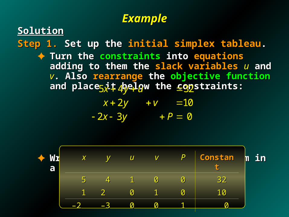
ExampleExampleSolutionSolutionStep 1.Step 1. Set up the Set up the initial simplex tableauinitial simplex tableau..
✦ Turn the Turn the constraintsconstraints into into equationsequations adding to them the adding to them the slack variablesslack variables uu and and vv. Also . Also rearrangerearrange the the objective objective functionfunction and place it below the constraints: and place it below the constraints:
✦ Write the Write the coefficientscoefficients of the system in a of the system in a tableautableau::
5 4 32
2 10
2 3 0
x y u
x y v
x y P
5 4 32
2 10
2 3 0
x y u
x y v
x y P
2 3Maximize P x y 2 3Maximize P x y xx yy uu vv PP ConstantConstant
55 44 11 00 00 3232
11 2 2 00 11 00 1010
––2 2 ––33 00 00 11 00
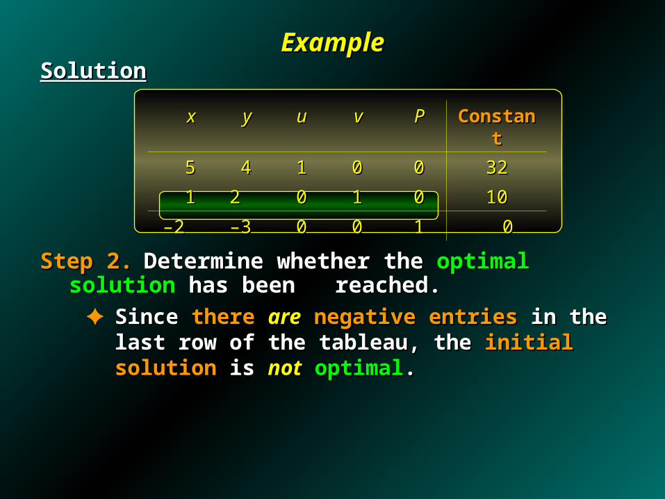
ExampleExampleSolutionSolution
Step 2.Step 2. Determine whether the Determine whether the optimal solutionoptimal solution has been has been reached.reached.
✦ Since Since there there areare negative entries negative entries in the last row of the in the last row of the tableau, the tableau, the initial solutioninitial solution is is notnot optimal optimal..
xx yy uu vv PP ConstantConstant
55 44 11 00 00 3232
11 2 2 00 11 00 1010
––2 2 ––33 00 00 11 00
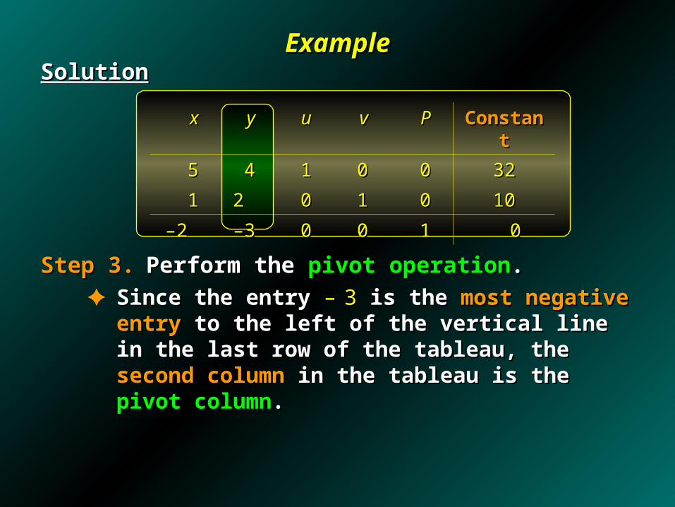
ExampleExampleSolutionSolution
Step 3.Step 3. Perform the Perform the pivot operationpivot operation..✦ Since the entry Since the entry –– 33 isis the the most negative entrymost negative entry to the left to the left
of the vertical line in the last row of the tableau, the of the vertical line in the last row of the tableau, the second columnsecond column in the tableau is the in the tableau is the pivot columnpivot column..
2 3Maximize P x y 2 3Maximize P x y xx yy uu vv PP ConstantConstant
55 44 11 00 00 3232
11 2 2 00 11 00 1010
––2 2 ––33 00 00 11 00

ExampleExampleSolutionSolution
Step 3.Step 3. Perform the Perform the pivot operationpivot operation..✦ Divide each Divide each positive numberpositive number of the of the pivot columnpivot column into the into the
corresponding entrycorresponding entry in the in the column of constantscolumn of constants and and compare the ratioscompare the ratios thus obtained. thus obtained.
✦ We see that the We see that the ratioratio 10/2 = 510/2 = 5 is is less thanless than the the ratio ratio 32/4 = 832/4 = 8, so , so row 2row 2 is the is the pivot rowpivot row..
2 3Maximize P x y 2 3Maximize P x y 324
102
8
5
324
102
8
5
xx yy uu vv PP ConstantConstant
55 44 11 00 00 3232
11 2 2 00 11 00 1010
––2 2 ––33 00 00 11 00
Ratio
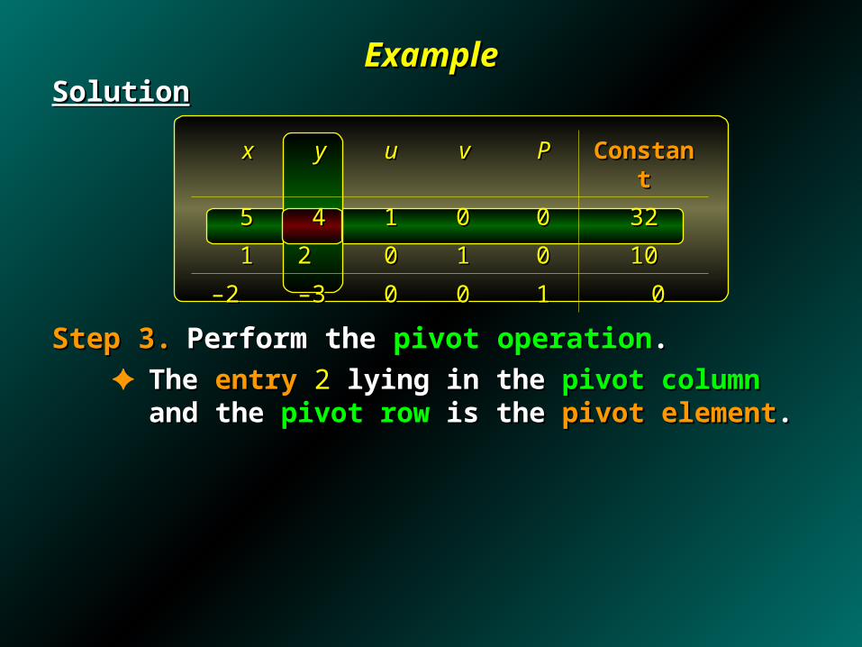
ExampleExampleSolutionSolution
Step 3.Step 3. Perform the Perform the pivot operationpivot operation..✦ The The entryentry 2 2 lying in the lying in the pivot columnpivot column and the and the pivot rowpivot row
is the is the pivot elementpivot element..
2 3Maximize P x y 2 3Maximize P x y xx yy uu vv PP ConstantConstant
55 44 11 00 00 3232
11 2 2 00 11 00 1010
––2 2 ––33 00 00 11 00

ExampleExampleSolutionSolution
Step 3.Step 3. Perform the Perform the pivot operationpivot operation..✦ Convert the Convert the pivot elementpivot element into a into a 1 1..
2 3Maximize P x y 2 3Maximize P x y xx yy uu vv PP ConstantConstant
55 44 11 00 00 3232
11 2 2 00 11 00 1010
––2 2 ––33 00 00 11 00
122 R122 R

ExampleExampleSolutionSolution
Step 3.Step 3. Perform the Perform the pivot operationpivot operation..✦ Convert the Convert the pivot elementpivot element into a into a 1 1..
2 3Maximize P x y 2 3Maximize P x y xx yy uu vv PP ConstantConstant
55 44 11 00 00 3232
1/21/2 1 1 00 1/21/2 00 55
––2 2 ––33 00 00 11 00
122 R122 R

ExampleExampleSolutionSolution
Step 3.Step 3. Perform the Perform the pivot operationpivot operation..✦ Use elementary Use elementary row operationsrow operations to convert the to convert the pivot pivot
columncolumn into a into a unit columnunit column..
2 3Maximize P x y 2 3Maximize P x y 1 2
3 2
4
3
R R
R R
1 2
3 2
4
3
R R
R R
xx yy uu vv PP ConstantConstant
55 44 11 00 00 3232
1/21/2 1 1 00 1/21/2 00 55
––2 2 ––33 00 00 11 00

ExampleExampleSolutionSolution
Step 3.Step 3. Perform the Perform the pivot operationpivot operation..✦ Use elementary Use elementary row operationsrow operations to convert the to convert the pivot pivot
columncolumn into a into a unit columnunit column..
2 3Maximize P x y 2 3Maximize P x y 1 2
3 2
4
3
R R
R R
1 2
3 2
4
3
R R
R R
xx yy uu vv PP ConstantConstant
33 00 11 ––22 00 1212
1/21/2 1 1 00 1/21/2 00 55
––1/2 1/2 00 00 3/23/2 11 1515

ExampleExampleSolutionSolution
Step 3.Step 3. Perform the Perform the pivot operationpivot operation..✦ This This completes an iterationcompletes an iteration..
✦ The The last rowlast row of the tableau contains a of the tableau contains a negative numbernegative number, , so an so an optimal solutionoptimal solution hashas notnot been reached been reached..
✦ Therefore, we Therefore, we repeatrepeat the the iteration stepiteration step..
2 3Maximize P x y 2 3Maximize P x y xx yy uu vv PP ConstantConstant
33 00 11 ––22 00 1212
1/21/2 1 1 00 1/21/2 00 55
––1/2 1/2 00 00 3/23/2 11 1515

ExampleExampleSolutionSolution
Step 3.Step 3. Perform the Perform the pivot operationpivot operation..✦ Since the entry Since the entry –1/2–1/2 isis the the most negative entrymost negative entry to the left to the left
of the vertical line in the last row of the tableau, the of the vertical line in the last row of the tableau, the first first columncolumn in the tableau is now the in the tableau is now the pivot columnpivot column..
2 3Maximize P x y 2 3Maximize P x y xx yy uu vv PP ConstantConstant
33 00 11 ––22 00 1212
1/21/2 1 1 00 1/21/2 00 55
––1/2 1/2 00 00 3/23/2 11 1515

ExampleExampleSolutionSolution
Step 3.Step 3. Perform the Perform the pivot operationpivot operation..✦ Divide each Divide each positive numberpositive number of the of the pivot columnpivot column into the into the
corresponding entrycorresponding entry in the in the column of constantscolumn of constants and and compare the ratioscompare the ratios thus obtained. thus obtained.
✦ We see that the We see that the ratioratio 12/3 = 412/3 = 4 is is less thanless than the the ratioratio 5/(1/2) = 105/(1/2) = 10, so , so row 1row 1 is now the is now the pivot rowpivot row..
2 3Maximize P x y 2 3Maximize P x y xx yy uu vv PP ConstantConstant
33 00 11 ––22 00 1212
1/21/2 1 1 00 1/21/2 00 55
––1/2 1/2 00 00 3/23/2 11 1515
123
51/2
4
10
123
51/2
4
10

ExampleExampleSolutionSolution
Step 3.Step 3. Perform the Perform the pivot operationpivot operation..✦ The The entryentry 3 3 lying in the lying in the pivot columnpivot column and the and the pivot rowpivot row
is the is the pivot elementpivot element..
xx yy uu vv PP ConstantConstant
33 00 11 ––22 00 1212
1/21/2 1 1 00 1/21/2 00 55
––1/2 1/2 00 00 3/23/2 11 1515
ExampleExampleSolutionSolution
Step 3.Step 3. Perform the Perform the pivot operationpivot operation..✦ Convert the Convert the pivot elementpivot element into a into a 1 1..
xx yy uu vv PP ConstantConstant
33 00 11 ––22 00 1212
1/21/2 1 1 00 1/21/2 00 55
––1/2 1/2 00 00 3/23/2 11 1515
113 R113 R
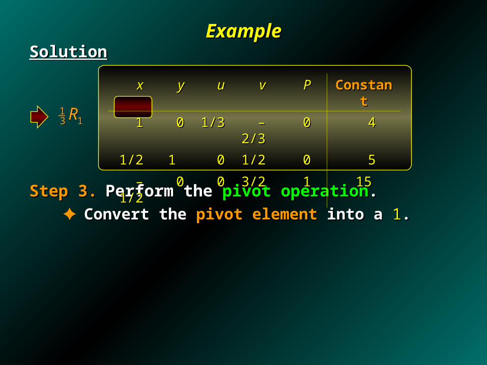
ExampleExampleSolutionSolution
Step 3.Step 3. Perform the Perform the pivot operationpivot operation..✦ Convert the Convert the pivot elementpivot element into a into a 1 1..
xx yy uu vv PP ConstantConstant
11 00 1/31/3 ––2/32/3 00 44
1/21/2 1 1 00 1/21/2 00 55
––1/2 1/2 00 00 3/23/2 11 1515
113 R113 R

ExampleExampleSolutionSolution
Step 3.Step 3. Perform the Perform the pivot operationpivot operation..✦ Use elementary Use elementary row operationsrow operations to convert the to convert the pivot pivot
columncolumn into a into a unit columnunit column..
12 12
13 12
R R
R R
12 12
13 12
R R
R R
xx yy uu vv PP ConstantConstant
11 00 1/31/3 ––2/32/3 00 44
1/21/2 1 1 00 1/21/2 00 55
––1/2 1/2 00 00 3/23/2 11 1515

ExampleExampleSolutionSolution
Step 3.Step 3. Perform the Perform the pivot operationpivot operation..✦ Use elementary Use elementary row operationsrow operations to convert the to convert the pivot pivot
columncolumn into a into a unit columnunit column..
12 12
13 12
R R
R R
12 12
13 12
R R
R R
xx yy uu vv PP ConstantConstant
11 00 1/31/3 ––2/32/3 00 44
00 1 1 ––1/61/6 5/65/6 00 33
00 00 1/61/6 7/67/6 11 1717

ExampleExampleSolutionSolution
Step 3.Step 3. Perform the Perform the pivot operationpivot operation..✦ The The last rowlast row of the tableau contains of the tableau contains nono negative negative
numbersnumbers, so an , so an optimal solutionoptimal solution has beenhas been reached reached..
xx yy uu vv PP ConstantConstant
11 00 1/31/3 ––2/32/3 00 44
00 1 1 ––1/61/6 5/65/6 00 33
00 00 1/61/6 7/67/6 11 1717

ExampleExampleSolutionSolution
Step 4.Step 4. Determine the Determine the optimal solutionoptimal solution..✦ Locate the Locate the basic variablesbasic variables in the final tableau. in the final tableau.
In this case, the In this case, the basic variablesbasic variables are are xx, , yy, and , and PP.. The The optimal valueoptimal value for for xx is is 44.. The The optimal valueoptimal value for for yy is is 33.. The The optimal valueoptimal value for for PP is is 1717, which means that , which means that
the the minimized valueminimized value for for CC is is –17–17..
xx yy uu vv PP ConstantConstant
11 00 1/31/3 ––2/32/3 00 44
00 1 1 ––1/61/6 5/65/6 00 33
00 00 1/61/6 7/67/6 11 1717
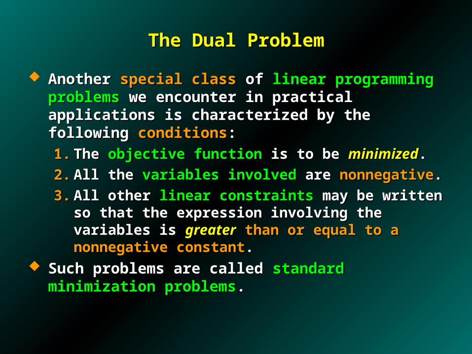
The Dual ProblemThe Dual Problem
Another Another special classspecial class of of linear programming problemslinear programming problems we we encounter in practical applications is characterized by the encounter in practical applications is characterized by the following following conditionsconditions::
1.1. The The objective functionobjective function is to be is to be minimizedminimized..
2.2. All the All the variables involvedvariables involved are are nonnegativenonnegative..
3.3. All other All other linear constraintslinear constraints may be written so that the may be written so that the expression involving the variables is expression involving the variables is greatergreater than or than or equal to a nonnegative constantequal to a nonnegative constant..
Such problems are called Such problems are called standard minimization standard minimization problemsproblems..

The Dual ProblemThe Dual Problem
In solving this kind of In solving this kind of linear programming problemlinear programming problem, it , it helps to note that each helps to note that each maximizationmaximization problemproblem is associated is associated with a with a minimizationminimization problemproblem, and vice versa., and vice versa.
The The given problemgiven problem is called the is called the primal problemprimal problem, and the , and the related problemrelated problem is called the is called the dual problemdual problem..

ExampleExample Write the Write the dual problemdual problem associated with this problem: associated with this problem:
We first write down a We first write down a tableautableau for the for the primal problemprimal problem::
6 8Minimize C x y 6 8Minimize C x y 40 10 2400
10 15 2100
5 15 1500
, 0
subject to x y
x y
x y
x y
40 10 2400
10 15 2100
5 15 1500
, 0
subject to x y
x y
x y
x y
xx yy ConstantConstant
4040 1010 24002400
1010 1515 21002100
55 1515 15001500
6 6 88
Primal Primal ProblemProblem
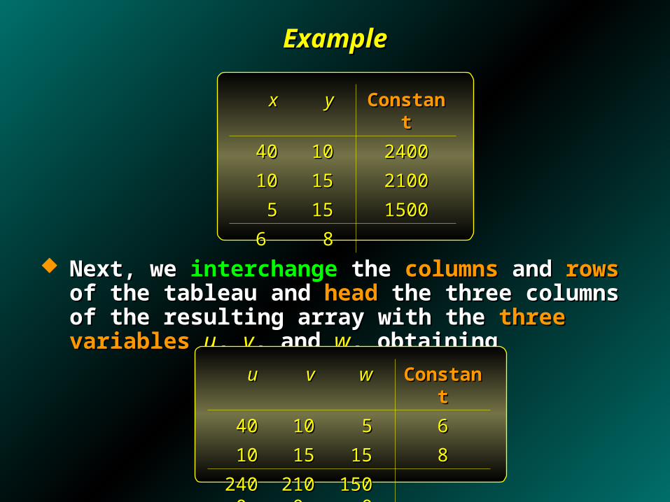
ExampleExample
Next, we Next, we interchangeinterchange the the columnscolumns and and rowsrows of the tableau of the tableau and and headhead the three columns of the resulting array with the the three columns of the resulting array with the three variablesthree variables uu, , vv, and , and ww, obtaining, obtaining
xx yy ConstantConstant
4040 1010 24002400
1010 1515 21002100
55 1515 15001500
6 6 88
uu vv ww ConstantConstant
4040 1010 55 66
1010 1515 1515 88
2400 2400 2100 2100 15001500

ExampleExample
Consider the resulting tableau as if it were the Consider the resulting tableau as if it were the initial initial simplex tableausimplex tableau for a for a standard maximization problemstandard maximization problem. .
From it we can reconstruct the required From it we can reconstruct the required dual problemdual problem::
uu vv ww ConstantConstant
4040 1010 55 66
1010 1515 1515 88
2400 2400 2100 2100 15001500
2400 2100 1500Maximize P u v w 2400 2100 1500Maximize P u v w
40 10 5 6
10 15 15 8
, , 0
subject to u v w
u v w
u v w
40 10 5 6
10 15 15 8
, , 0
subject to u v w
u v w
u v w
Dual Dual ProblemProblem
Theorem 1Theorem 1
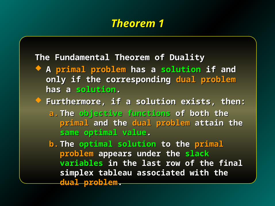
The Fundamental Theorem of DualityThe Fundamental Theorem of Duality A A primal problemprimal problem has a has a solutionsolution if and only if the if and only if the
corresponding corresponding dual problemdual problem has a has a solutionsolution.. Furthermore, if a solution exists, then:Furthermore, if a solution exists, then:
a.a. The The objective functionsobjective functions of both the of both the primalprimal and and the the dual problemdual problem attain the attain the same optimal valuesame optimal value..
b.b. The The optimal solutionoptimal solution to the to the primal problemprimal problem appears under the appears under the slack variablesslack variables in the last row in the last row of the final simplex tableau associated with the of the final simplex tableau associated with the dual problemdual problem..
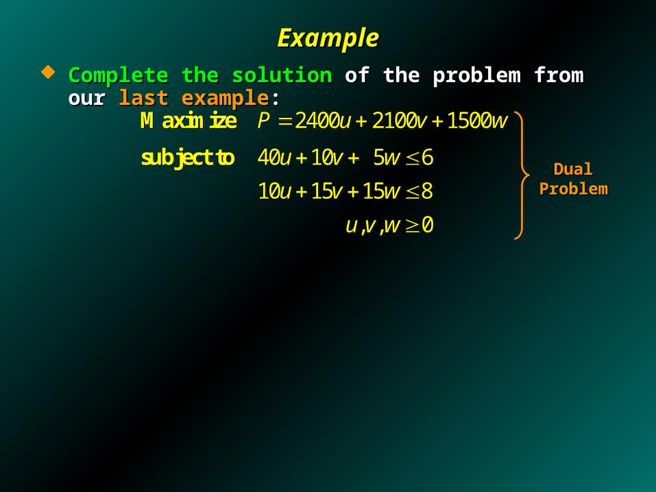
ExampleExample Complete the solutionComplete the solution of the problem from our of the problem from our last examplelast example::
2400 2100 1500Maximize P u v w 2400 2100 1500Maximize P u v w
40 10 5 6
10 15 15 8
, , 0
subject to u v w
u v w
u v w
40 10 5 6
10 15 15 8
, , 0
subject to u v w
u v w
u v w
Dual Dual ProblemProblem
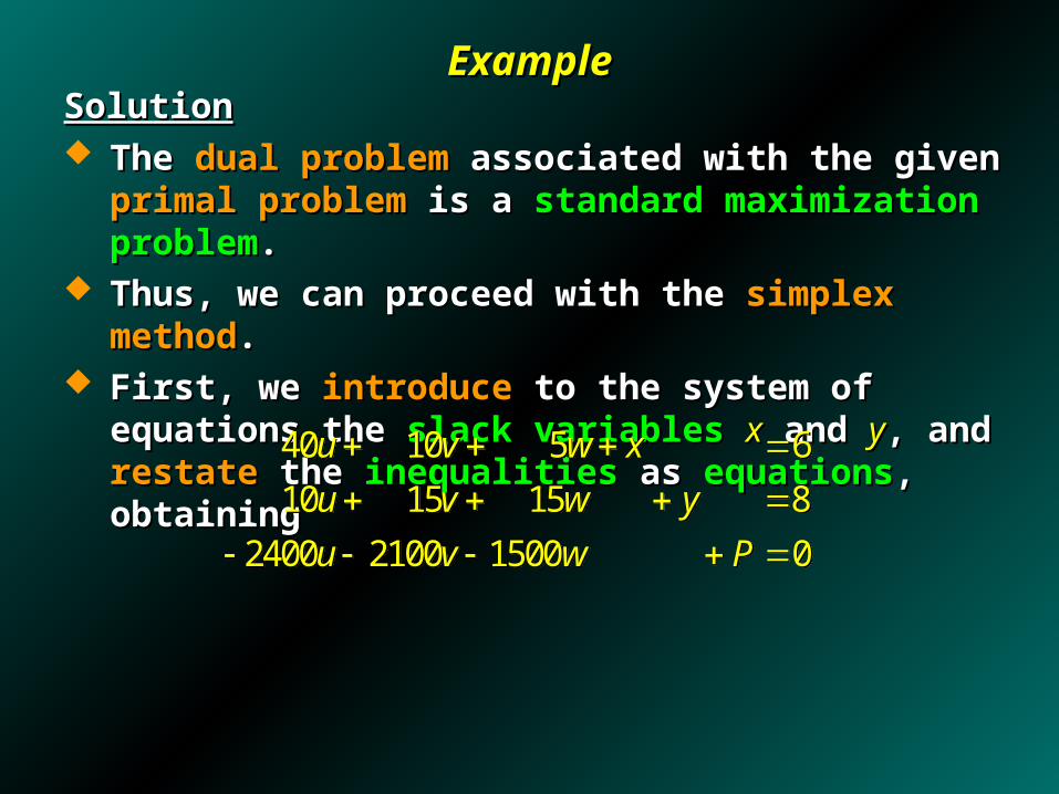
ExampleExampleSolutionSolution The The dual problemdual problem associated with the given associated with the given primal primal
problemproblem is a is a standard maximization problemstandard maximization problem.. Thus, we can proceed with the Thus, we can proceed with the simplex methodsimplex method.. First, we First, we introduceintroduce to the system of equations the to the system of equations the slack slack
variablesvariables xx and and yy, and , and restaterestate the the inequalitiesinequalities as as equationsequations, , obtainingobtaining
40 10 5 6
10 15 15 8
2400 2100 1500 0
u v w x
u v w y
u v w P
40 10 5 6
10 15 15 8
2400 2100 1500 0
u v w x
u v w y
u v w P
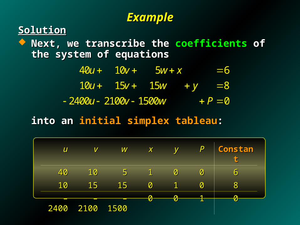
ExampleExampleSolutionSolution Next, we transcribe the Next, we transcribe the coefficientscoefficients of the system of of the system of
equations equations
into an into an initial simplex tableauinitial simplex tableau::
40 10 5 6
10 15 15 8
2400 2100 1500 0
u v w x
u v w y
u v w P
40 10 5 6
10 15 15 8
2400 2100 1500 0
u v w x
u v w y
u v w P
uu vv ww xx yy PP ConstantConstant
4040 1010 55 11 00 00 66
1010 1515 1515 00 11 00 88
––2400 2400 ––2100 2100 ––15001500 00 00 11 00
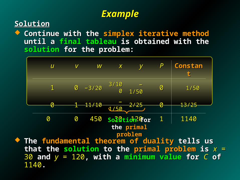
ExampleExampleSolutionSolution Continue with the Continue with the simplex iterative methodsimplex iterative method until a until a final final
tableautableau is obtained with the is obtained with the solutionsolution for the problem: for the problem:
The The fundamental theorem of dualityfundamental theorem of duality tells us that the tells us that the solutionsolution to the to the primal problemprimal problem is is xx = 30 = 30 and and yy = 120 = 120, with a , with a minimum valueminimum value for for CC of of 11401140..
uu vv ww xx yy PP ConstantConstant
11 00 ––3/203/20 3/1003/100 ––1/501/50 00 1/501/50
00 11 11/1011/10 ––1/501/50 2/252/25 00 13/2513/25
0 0 00 450450 3030 120120 11 11401140
SolutionSolution for thefor the primal problemprimal problem
End of End of Chapter Chapter