6 designing engineering systems for sustainability

6

Designing Engineering Systems for Sustainability

Peter Sandborn and Jessica Myers CALCE, Department of Mechanical Engineering, University of Maryland

Abstract

Sustainability means keeping an existing system operational and maintaining the ability to manufacture and field versions of the system that satisfy the original requirements. Sustainability also includes manufacturing and fielding revised versions of the system that satisfy evolving requirements, which often requires the replacement of technologies used in the original system with newer technologies. Technology sustainment analysis encompasses the ramifications of reliability on system management and costs via sparing, availability and warranty. Sustainability also requires the management of technology obsolescence (forecasting, mitigation and strategic planning) and addresses roadmapping, surveillance, and value metrics associated with technology insertion planning. 6.1 Introduction

The word ‘sustain’ has comes from the Latin sustenare meaning "to hold up" or to support, which has evolved to mean keeping something going or extending its duration, [6.1]. The most common non-specialized synonym for sustain is ‘maintain’. Although maintain and sustain are sometimes used interchangeably, maintenance usually refers to activities targeted at correcting problems, and sustainment is a more general term referring to the management of system evolution.

Sustainability can mean static equilibrium (the absence of change) or dynamic equilibrium (constant, predictable or manageable change), [6.2]. The most widely circulated definition of sustainability (or more accurately sustainable development) is attributed to the Brundtland Report [6.3], which is often stated as “development that meets the needs of present generations without compromising the ability of future generations to meet their own needs.” Although this definition was created in the context of environmental sustainability, it is useful for defining all types of sustainability. Although the concept of sustainability appears throughout nearly all disciplines; we will only mention the most prevalent usages here: Environmental Sustaintability – the ability of an ecosystem to maintain ecological processes and functions, biological diversity, and productivity over time, [6.4]. The objective of environmental sustainability is to increase energy and material efficiencies, preserve ecosystem integrity, and promote human health and happiness by merging design, economics, manufacturing and policy.

Business or Corporate Sustainability – the increase in productivity and/or reduction of consumed resources without compromising product or service quality, competitiveness, or profitability. Business sustainability is often described as the triple bottom line (3BL) [6.5]: financial (profit), social (people) and environmental (planet). A closely related

Designing Engineering Systems for Sustainment

endeavor is “sustainable operations management”, which integrates profit and efficiency with the company’s stakeholders and the resulting environmental impacts, [6.6]. Technology Sustainment - all activities necessary to: a) keep an existing system operational (able to successfully complete its intended purpose); b) continue to manufacture and field versions of the system that satisfy the original requirements; and c) manufacture and field revised versions of the system that satisfy evolving requirements. The term “sustainment engineering” is sometimes applied to technology sustainment activities and is the process of assessing and improving a system’s ability to be sustained by determining, selecting and implementing feasible and economically viable alternatives, [6.7]. For technology sustainment, “present and future generations” in the Brundtland definition can be interpreted as the users and maintainers of a system.

This chapter focuses on the specific and unique activities associated with technology sustainability.

Sustainment-Dominated Systems

In the normal course of product development, it often becomes necessary to change the design of products and systems consistent with shifts in demand and with changes in the availability of the materials and components from which they are manufactured. When the content of the system is technological in nature, the short product life cycle associated with fast moving technology changes becomes both a problem and an opportunity for manufacturers and systems integrators.

For most high-volume, consumer oriented products and systems; the rapid rate of technology change translates into a critical need to stay on the leading edge of technology. These product sectors must adapt the newest materials, components, and processes in order to prevent loss of their market share to competitors. For leading-edge products, updating the design of a product or system is a question of balancing the risks of investing resources in new, potentially immature technologies against potential functional or

performance gains that could differentiate them from their competitors in the market. Examples of leading-edge products that race to adapt to the newest technology are high-volume consumer electronics, e.g., mobile phones and PDAs.

There are however, significant product sectors that find it difficult to adopt leading-edge technology. Examples include: airplanes, ships, computer networks for air traffic control and power grid management, industrial equipment, and medical equipment. These product sectors often “lag” the technology wave because of the high costs and/or long times associated with technology insertion and design refresh. Many of these product sectors involve “safety critical” systems where lengthy and expensive qualification/ certification cycles may be required even for minor design changes and where systems are fielded (and must be maintained) for long periods of time (often 20 years or more). Because of these attributes, many of these product sectors also share the common attribute of being “sustainment-dominated”, i.e., their long-term sustainment (life cycle) costs exceed the original procurement costs for the system.

Some types of sustainment-dominated systems are obvious, e.g., Figure 6.1 shows the life cycle cost breakdown for an F-16 military aircraft where only 22% of the life cycle cost of the system is associated with design, development and manufacturing (this 22% also includes deployment, training, and initial spares). The other 78% is operation and support and includes all costs of operating, maintaining, and supporting, i.e., costs for personnel; consumable and repairable materials; organizational, intermediate and depot

R&D2%

Investment20%

Sustainment78%

Figure 6.1. Cost breakdown for an F-16, [6.8]

Technology Sustainment 83

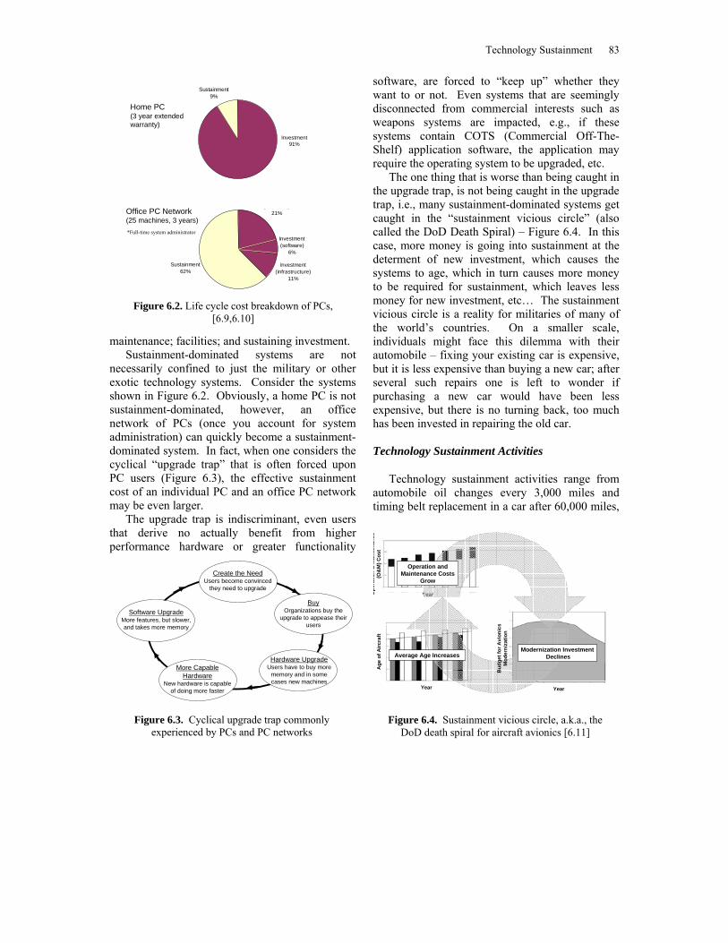
maintenance; facilities; and sustaining investment. Sustainment-dominated systems are not

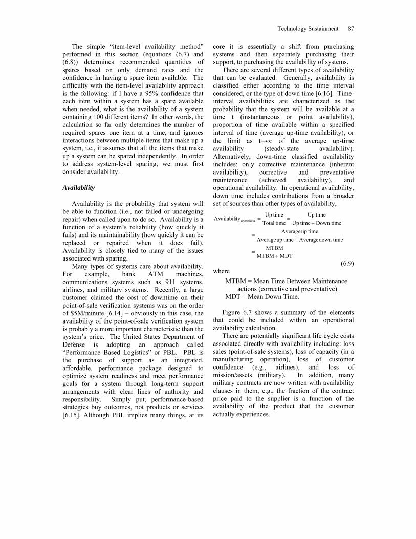
necessarily confined to just the military or other exotic technology systems. Consider the systems shown in Figure 6.2. Obviously, a home PC is not sustainment-dominated, however, an office network of PCs (once you account for system administration) can quickly become a sustainment-dominated system. In fact, when one considers the cyclical “upgrade trap” that is often forced upon PC users (Figure 6.3), the effective sustainment cost of an individual PC and an office PC network may be even larger.

The upgrade trap is indiscriminant, even users that derive no actually benefit from higher performance hardware or greater functionality

software, are forced to “keep up” whether they want to or not. Even systems that are seemingly disconnected from commercial interests such as weapons systems are impacted, e.g., if these systems contain COTS (Commercial Off-The-Shelf) application software, the application may require the operating system to be upgraded, etc.

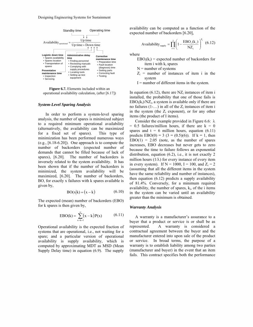
The one thing that is worse than being caught in the upgrade trap, is not being caught in the upgrade trap, i.e., many sustainment-dominated systems get caught in the “sustainment vicious circle” (also called the DoD Death Spiral) – Figure 6.4. In this case, more money is going into sustainment at the determent of new investment, which causes the systems to age, which in turn causes more money to be required for sustainment, which leaves less money for new investment, etc… The sustainment vicious circle is a reality for militaries of many of the world’s countries. On a smaller scale, individuals might face this dilemma with their automobile – fixing your existing car is expensive, but it is less expensive than buying a new car; after several such repairs one is left to wonder if purchasing a new car would have been less expensive, but there is no turning back, too much has been invested in repairing the old car. Technology Sustainment Activities

Technology sustainment activities range from automobile oil changes every 3,000 miles and timing belt replacement in a car after 60,000 miles,

Software UpgradeMore features, but slower, and takes more memory

Create the NeedUsers become convinced

they need to upgrade

BuyOrganizations buy the

upgrade to appease their users

Hardware UpgradeUsers have to buy more

memory and in some cases new machines

More CapableHardware

New hardware is capableof doing more faster

Figure 6.3. Cyclical upgrade trap commonly

experienced by PCs and PC networks

Investment (hardware)

21%

Investment (software)

6%

Investment (infrastructure)

11%

Sustainment62%

*Full-time system administrator

Investment91%

Sustainment9%

Office PC Network (25 machines, 3 years)

Home PC(3 year extended warranty)

Investment91%

Figure 6.2. Life cycle cost breakdown of PCs,

[6.9,6.10]

Ope

ratio

n &

Mai

nten

ance

(O

&M

) Cos

t

YearYear

Bud

get f

or A

vion

ics

Mod

erni

zatio

n

Year

Age

of A

ircra

ft

Modernization InvestmentDeclinesAverage Age Increases

Operation and Maintenance Costs

Grow

Figure 6.4. Sustainment vicious circle, a.k.a., the

DoD death spiral for aircraft avionics [6.11]


to warranty repair of a television and scheduled maintenance of a commercial aircraft engine. There are also less obvious sustainment activities that include time spent with technical support provided by a PC manufacturer via telephone or email, installation of an operating system upgrade, or addition of memory to an existing PC to support a new version of application software. The various elements involved in sustainment include:

• Reliability • Obsolescence • Testability • Warranty/Guarantee • Diagnosibility • Qualification/Certification • Repairability • Configuration Control • Maintainability • Regression Testing • Spares • Upgradability • Availability • Total Cost of Ownership • Cross-Platform

Applicability • Technology

Infusion/Insertion Obviously, the relevancy of sustainment

activities varies depending on the type of system. For “throw-away” products such as a computer mouse or keyboard, sustainment primarily translates into warranty replacement. For consumer electronics, such as televisions, sustainment is dominated by repair or warranty replacement upon failure. Demand-critical electronics (availability sensitive systems), such as ATM machines and servers, include some preventative maintenance, upgrades, repair upon failure, and sparing. Long field life electronics, such as avionics and military systems, are aggressively maintained, have extensive built in test and diagnosis, are repaired at several different levels, and are continuously upgraded.

This chapter cannot practically cover all the

topics that make up technology sustainment. We will not focus on reliability (reliability is the topic of many books and addressed in several other chapters within this book). We will also not focus on testability or diagnosability since these are also the topics of other books and journals. Rather, we will concentrate on the ramifications of reliability on system management and costs via sparing, availability and warranty (Section 6.2). Section 6.3 treats technology obsolescence and discusses

forecasting, mitigation and strategic planning. Section 6.4 addresses technology insertion. 6.2 Sparing and Availability

Reliability is possibly the most important attribute of a system. Without reliability, the value derived from performance, functionality, or low cost cannot be realized. The ramifications of reliability on the system life cycle management are linked to life cycle cost through sparing requirements and warranty return rates, and measured by system availability.

Reliability is the probability that an item will not fail. Maintainability is the probability that the item can be successfully restored to operation after failure; and availability provides information about how efficiently the system is managed and is a function of reliability and maintainability.

Item-Level Sparing Analysis

When a system encounters a failure, one of the following things happens: • Nothing happens – a workaround for the failure

is implemented and operation continues or the system is disposed of and the functionality or role that the system performed is accomplished another way or deleted.

• The system is repaired – if your car has a flat tire, you don’t dispose of the car, and you may not dispose of the tire either, you fix the tire.

• The system is replaced – at some level, repair is impractical and the failing portion of the system is replaced; if an IC in your stereo fails, you can’t repair a problem inside the IC, you have to replace the IC. If a tire on your car blows out on the highway

and is damaged to such an extent that it cannot be repaired, you have to replace it. What do you replace the flat tire with? If you have a replacement (spare) in your trunk, you can change the tire and be on your way quickly. If you don’t have a replacement you have to either have a replacement brought to the car or you have to have the car towed to someplace that has a replacement. If no one has a replacement, someone has to manufacture one for you.


Spare tires exist and are carried in cars because the “availability” of a car is important to the car’s driver, i.e., having your car unavailable to you because no spare tire exists is a problem, you can’t get to work, you can’t take the kids to school, etc. If you are an airline, having an airplane unavailable to carry passengers (thus not earning revenue) because a spare part does not exist or is in the wrong location can be a very costly problem. Therefore, spares are manufactured and available for use for many types of systems.

There are several issues with spares that make sparing analysis challenging: • How many spares do you need to have? I don’t

want to manufacture 1000 spares if I will only need 200 to keep the system operational (available) at the required rate.

• When are you going to need the spares? The number of spares I need is a function of time (or miles, or other accumulated environmental stresses), i.e., as systems age, the number of spares needed may increase. When should I manufacture the spares (with the original production or later)? What if I run out and have to manufacture more spares?

• Where should the spares be kept? Spares need to be available where systems fail, not 3000 miles away. When I have a flat tire, is a spare tire more useful in my garage or in the trunk of my car?

• What level (in a system) do you want to spare at? It makes sense to carry a spare tire in my trunk, but it does not make sense to carry a spare transmission in the trunk, why? Because transmissions do not fail as frequently as tires, transmissions are large and heavy to carry, and I don’t have the tools, or expertise to install a new transmission on the side of the road.

Spare part quantities are a function of demand rates and are expected to [6.12]: • Cover actual item replacements occurring as a

result of corrective and preventative maintenance actions

• Compensate for repairable items in the process of undergoing maintenance

• Compensate for the procurement lead times required for replacement item acquisition

• Compensate for the condemnation or scrapage of repairable items. In order to explore how spare quantities are

determined, we first need to review simple reliability calculations. Reliability is given in terms of time (t) by,

∫−=t

0

f(t)dt1R(t) (6.1)

The reliability, R(t), is the probability of no failures in time t. If the time to failure, f(t), follows an exponential distribution,

λtλef(t) −= (6.2)

where λ is the failure rate (λ = 1/MTBF, MTBF = Mean Time Between Failure), then the reliability becomes,

λtt

0

λtt

0

λt ee1dtλe1R(t) −−− =+=−= ∫ (6.3)

Equation (6.3) is the probability of exactly 0 failures in time t. This result can be generalized to give the probability of exactly x failures in time t is given by,

( )x!

eλtP(x)λtx −

= (6.4)

So, for x = 0, λteP(0) −= (the result in (6.3)), for x = 1, λtλteP(1) −= , etc. For a unique system with no spares, the probability of surviving to time t is P(0). For a unique system with exactly one spare available, the probability of surviving to time t is given by,

( ) ( ) λtλt λtee1P0P −− +=+ (6.5)

or in general,

( )∑=

−

=≤k

0x

λtx

x!eλtk)P(x (6.6)


Equation (6.6) is the cumulative Poisson probability, i.e., the probability of k or fewer failures in time t. This is the probability of surviving to time t with k spares, or, k is the minimum number of spares needed in order to have a confidence level of P(x ≤ k) that the system will survive to time t.

The derivation of equation (6.6) assumes that there is only one instance of the spared item in service, if there are n instances in service, then equation (6.6) becomes [6.13],

( )∑=

−

=≤k

0x

λtn x

x!e tnλk)P(x (6.7)

where, k = number of spares n = number of unduplicated (in series, not

redundant) units in service λ = constant failure rate (exponential

distribution of time to failure) of the unit or the average number of maintenance events expected to occur in time t

t = given time interval P(x ≤ k) = probability that k is enough spares

or the probability that a spare will be available when needed

nλt = system unavailability. When k is large, the Poisson distribution can be approximated by the normal distribution and k can be approximately calculated in closed form,

⎡ ⎤λt zλt k +≅ (6.8)

where z is the number of standard deviations from the mean of a standard normal distribution, Figure

6.5. Equation (6.8) is only applicable when times between failures are exponentially distributed, and the recovery/repair times are independent and exponentially distributed.

Figure 6.6 shows a simple example sparing calculation performed using equations (6.7) and (6.8). For the example data shown in Figure 6.6 a simple approximation for the number of required spares is: the MTBF = 1/λ = 2x106 hours and the unit has to be supported for t = 1500 hours; 1500/2x106 = 0.0008 spares per unit; therefore, for n = 25,000 units, the total number of spares needed is (25000)(0.0008) = 18.75. Rounding up to19 spares, Figure 6.6 indicates that for the simple approximation, there is a 58% confidence that 19 are enough spares to last 1500 hours.

There are several costs associated with carrying spares: • Cost of manufacturing spares • Cost of money tied up in manufactured spares

for future use – spares for the future may have to be made now before the required components become obsolete (see Section 6.3)

• Cost of transporting spares to where they are needed (or conversely the cost of transporting the system to the location where the spares are kept)

• Cost of storing spares until needed • Cost of replenishing spares if they run out • Cost of system availability impacts due to spares

not being in the right place at the right time.

0.0000

0.2000

0.4000

0.6000

0.8000

1.0000

1.2000

0 10 20 30 40

k (number of spares)

Con

fiden

ce L

evel

(fra

ctio

n)

Poisson DistributionNormal Distribution Approx.

Figure 6.6. Sparing calculation for n = 25000, t = 1500 hours, and λ = 0.5 failures/million hours

Prob

abili

ty

areaz

area = confidence level desired

Example:confidence level = 95%, z = 1.645 confidence level = 90%, z = 1.282confidence level = 50%, z = 0

0

Normal distribution

Figure 6.5. Relationship between z and confidence level


The simple “item-level availability method” performed in this section (equations (6.7) and (6.8)) determines recommended quantities of spares based on only demand rates and the confidence in having a spare item available. The difficulty with the item-level availability approach is the following: if I have a 95% confidence that each item within a system has a spare available when needed, what is the availability of a system containing 100 different items? In other words, the calculation so far only determines the number of required spares one item at a time, and ignores interactions between multiple items that make up a system, i.e., it assumes that all the items that make up a system can be spared independently. In order to address system-level sparing, we must first consider availability.

Availability

Availability is the probability that system will be able to function (i.e., not failed or undergoing repair) when called upon to do so. Availability is a function of a system’s reliability (how quickly it fails) and its maintainability (how quickly it can be replaced or repaired when it does fail). Availability is closely tied to many of the issues associated with sparing.

Many types of systems care about availability. For example, bank ATM machines, communications systems such as 911 systems, airlines, and military systems. Recently, a large customer claimed the cost of downtime on their point-of-sale verification systems was on the order of $5M/minute [6.14] – obviously in this case, the availability of the point-of-sale verification system is probably a more important characteristic than the system’s price. The United States Department of Defense is adopting an approach called “Performance Based Logistics” or PBL. PBL is the purchase of support as an integrated, affordable, performance package designed to optimize system readiness and meet performance goals for a system through long-term support arrangements with clear lines of authority and responsibility. Simply put, performance-based strategies buy outcomes, not products or services [6.15]. Although PBL implies many things, at its

core it is essentially a shift from purchasing systems and then separately purchasing their support, to purchasing the availability of systems.

There are several different types of availability that can be evaluated. Generally, availability is classified either according to the time interval considered, or the type of down time [6.16]. Time-interval availabilities are characterized as the probability that the system will be available at a time t (instantaneous or point availability), proportion of time available within a specified interval of time (average up-time availability), or the limit as t→∞ of the average up-time availability (steady-state availability). Alternatively, down-time classified availability includes: only corrective maintenance (inherent availability), corrective and preventative maintenance (achieved availability), and operational availability. In operational availability, down time includes contributions from a broader set of sources than other types of availability,

MDTMTBMMTBM

down time Average timeup Average timeup Average

Down time timeUp timeUp

timeTotal timeUptyAvailabili loperationa

+=

+=

+==

(6.9) where

MTBM = Mean Time Between Maintenance actions (corrective and preventative)

MDT = Mean Down Time. Figure 6.7 shows a summary of the elements

that could be included within an operational availability calculation.

There are potentially significant life cycle costs associated directly with availability including: loss sales (point-of-sale systems), loss of capacity (in a manufacturing operation), loss of customer confidence (e.g., airlines), and loss of mission/assets (military). In addition, many military contracts are now written with availability clauses in them, e.g., the fraction of the contract price paid to the supplier is a function of the availability of the product that the customer actually experiences.


System-Level Sparing Analysis

In order to perform a system-level sparing analysis, the number of spares is minimized subject to a required minimum operational availability (alternatively, the availability can be maximized for a fixed set of spares). This type of minimization has been performed numerous ways (e.g., [6.18-6.20]). One approach is to compute the number of backorders (expected number of demands that cannot be filled because of lack of spares), [6.20]. The number of backorders is inversely related to the system availability. It has been shown that if the number of backorders is minimized, the system availability will be maximized, [6.20]. The number of backorders, BO, for exactly x failures with k spares available is given by, ( )kxk)xBO( −= (6.10)

The expected (mean) number of backorders (EBO) for k spares is then given by,

( )P(x) kxEBO(k)1kx

∑∞

+=

−= (6.11)

Operational availability is the expected fraction of systems that are operational, i.e., not waiting for a spare; and a particular version of operational availability is supply availability, which is computed by approximating MDT as MSD (Mean Supply Delay time) in equation (6.9). The supply

availability can be computed as a function of the expected number of backorders [6.20],

∏=

⎟⎟⎠

⎞⎜⎜⎝

⎛−=

I

1i

Z

i

iisupply

i

NZ)(kEBO

1tyAvailabili (6.12)

where EBOi(ki) = expected number of backorders for

item i with ki spares N = number of systems Zi = number of instances of item i in the

system I = number of different items in the system.

In equation (6.12), there are NZi instances of item i installed, the probability that one of those fails is EBOi(ki)/NZi, a system is available only if there are no failures (1-…) in all of the Zi instances of item i in the system (the Zi exponent), or for any other items (the product of I items).

Consider the example provided in Figure 6.6: λ = 0.5 failures/million hours, if there are k = 0 spares and t = 6 million hours, equation (6.11) predicts EBO(0) = 3 (3 = (0.5)(6)). If k = 1, then EBO(1) = 2.05 (note, as the number of spares increases, EBO decreases but never gets to zero because the time to failure follows an exponential distribution, equation (6.2), i.e., it is not exactly 2 million hours (1/λ) for every instance of every item in every system). If N = 1000, I = 100, and Zi = 2 (assuming that all the different items in the system have the same reliability and number of instances), then equation (6.12) predicts a supply availability of 81.4%. Conversely, for a minimum required availability, the number of spares, ki, of the i items in the system can be varied until an availability greater than the minimum is obtained.

Warranty Analysis

A warranty is a manufacturer’s assurance to a buyer that a product or service is or shall be as represented. A warranty is considered a contractual agreement between the buyer and the manufacturer entered into upon sale of the product or service. In broad terms, the purpose of a warranty is to establish liability among two parties (manufacturer and buyer) in the event that an item fails. This contract specifies both the performance

Down time timeUp timeUptyAvailabili loperationa +

=

Standby time Operating time

Logistic down time• Spares availability• Spares location• Transportation of

spares

Administrative delay time• Finding personnel• Reviewing manuals• Complying with

supply procedures• Locating tools• Setting up test

equipment

Corrective maintenance time• Preparation time• Fault location

(diagnosis) time• Getting parts• Correcting fault• Testing

Preventative maintenance time• Inspection• Servicing

Figure 6.7. Elements included within an

operational availability calculation, (after [6.17])


that is to be expected and the redress available to the buyer if a failure occurs, [6.21].

Warranty cost analysis is performed to estimate the cost of servicing a warranty (so that it can be properly accounted for in the sales price or maintenance contract for the system). Similar to sparing analysis, warranty analysis is focused on determining the number of expected system failures during some period of operation (the warranty period) that will result in a warranty action. Unlike, sparing analysis, warranty analysis does not base its sparing needs on maintaining a specific system availability, but only servicing all the warranty claims.

Warranties do not assume that failed items need to be replaced (they may be repairable). Those items that are not repairable need replacement and therefore need spares. Spares may also be needed as “loaners” during system repair.

Warranty analysis differs from sparing in two basic ways. First, warranty analysis usually aims to determine a warranty reserve cost (the total amount of money that has to be reserved to cover the warranty on a product). The cost of servicing an individual warranty claim may vary depending on the type of warranty provided. The simplest case is an unlimited free replacement warranty in which every failure prior to the end of the warranty period is replaced or repaired to its original condition at no charge to the customer. In this case, the warranty reserve fund (ignoring the cost of money) is given by, ( )cfrwr kCCnC += (6.13)

where, n = quantity of product sold Cfr = fixed cost (per product instance) of

providing warranty coverage Cc = recurring replacement/repair cost per

produce instance k = number of warranty actions, i.e., wλT≅

or determined from equations (6.7) or (6.8)

Tw = length of the warranty.

Other types of warranties also exist. For example some warranties are pro-rata – whenever a product fails prior to the end of the warranty

period, it is replaced at a cost that is a function of the item’s age at the time of failure. If θ is the product price including the warranty then (following a linear depreciation with time),

⎟⎟⎠

⎞⎜⎜⎝

⎛−

wTt1θ is the amount of money rebated to a

customer for a failure at time t. In this case, the total cost of servicing the warranty assuming a constant failure rate is given by,

( )⎟⎟⎠

⎞⎜⎜⎝

⎛−−=⎟⎟

⎠

⎞⎜⎜⎝

⎛−= −−∫ w

wλT

w

T

0

λt

wwr e1

λT11nθdte nλ

Tt1θC .

(6.14) Consider a manufacturer of television sets who

is going to provide a 12 month pro-rata warranty. The failure rate of the televisions is λ = 0.004 failures per month, n = 500,000, the desired profit margin is 8%, and the recurring cost per television is $112; what warranty reserve fund should be put in place? From equation (6.14), Cwr/θ = 11,800. Assuming that the profit margin is on the recurring cost of the television and its effective warranty cost, θ is given by,

( ) ⎟⎠⎞

⎜⎝⎛ ++=

nC

cost recurring1 margin profit θ wr ,

(6.15) solving for Cwr gives $1,464,659, or $2.93/television to cover warranty costs.

The warranty reserve funds computed in equations (6.13) and (6.14) assume that every warranty action is solved by replacement of the defective product with a new item. If the defective product can be repaired, than other variations on simple warranties can be derived, see [6.22].

A second way that warranties differ from sparing analysis is that the period of performance (the period in which expected failures need to be counted) can be defined in a more complex way. For example, two-dimensional warranties are common in the automotive industry – 3 years or 36,000 miles, whichever comes first. A common way to represent a two-dimensional warranty is shown in Figure 6.8. Note, many other more complexly shaped two-dimensional warranty


schemes are possible, see [6.23]. In Figure 6.8, W is the warranty period and U is the usage limit, i.e., unlimited free replacement up to time W or usage U, whichever occurs first from the time of initial purchase. r is called the usage rate (usage per unit time). The warranty ends at U (if r ≥ γ1) or W (if r < γ1). Every failure that falls within the rectangle defined by U and W requires a warranty action. As a result, modeling the number of failures that require warranty actions involves either a bivariate failure model (e.g., [6.23]), or a univariate model that incorporates the usage rate appropriately (e.g., [6.24]). 6.3 Technology Obsolescence

A significant problem facing many “high-tech” sustainment-dominated systems is technology obsolescence, and no technology typifies the problem more than electronic part obsolescence, where electronic parts refers to integrated circuits and discrete passive components. In the past several decades, electronic technology has advanced rapidly causing electronic components to have a shortened procurement life span, e.g., Figure 6.9. QTEC estimates that approximately 3% of the global pool of electronic components goes obsolete every month, [6.26]. Driven by the consumer electronics product sector, newer and better electronic components are being introduced frequently, rendering older components obsolete. Yet, sustainment-dominated systems such as aircraft avionics are often produced for many years and sustained for decades. In particular, sustainment-dominated products suffer the

consequences of electronic part obsolescence because they have no control over their electronic part supply chain due to their low production volumes. The obsolescence problem for sustainment-dominated systems is particularly troublesome since they are often subject to significant qualification/certification requirements that can make even simple changes to a system prohibitively expensive. This problem is especially prevalent in avionics and military systems, where systems often encounter obsolescence problems before they are fielded and always during their support life, e.g., Figure 6.10.

Obsolescence, also called DMSMS – Diminishing Manufacturing Sources and Material Shortages, is defined as the loss or impending loss of original manufacturers of items or suppliers of items or raw materials. The key defining characteristic of obsolescence problems is that the products are forced to change (even though they may not need to or want to change) by circumstances that are beyond their control. The type of obsolescence addressed here is caused by the unavailability of technologies (parts) that are needed to manufacture or sustain a product. A different type of obsolescence called “sudden obsolescence” or “inventory obsolescence” refers to the opposite problem in which inventories of parts become obsolete because the system they

W

U

γ1 = U/W

r = γ1

r < γ1

r ≥ γ1

Time or Age

Usa

ge

Figure 6.8. A representation of a two-dimensional

free-replacement warranty policy 0

4

8

12

16

20

24

28

32

36

1969 1974 1979 1984 1989 1994 1999 2004

Introduction Year

Proc

urem

ent L

ifetim

e (y

ears

)

Figure 6.9. Decreasing procurement lifetime for

operational amplifiers, [6.25]. The procurement life is the number of years the part can be procured from

its original manufacturer


were being saved for changes so that the inventories are no longer required, e.g., [6.27].

Electronic Part Obsolescence

Electronic part obsolescence began to emerge as a problem in the 1980s when the end of the Cold War accelerated pressure to reduce military outlays and lead to an effort in the United States military called Acquisition Reform. Acquisition reform included a reversal of the traditional reliance on military specifications (“Mil-Specs”) in favor of commercial standards and performance specifications [6.28]. One of the consequences of the shift away from Mil-Specs was that Mil-Spec parts that were qualified to more stringent environmental specifications than commercial parts and manufactured over longer-periods of time were no longer available, creating the necessity to use Commercial Off The Shelf (COTS) parts that are manufactured for non-military applications and, by virtue of their supply chains being controlled by commercial and consumer products, are usually procurable for much shorter periods of time. Although this history is associated with the military, the problem it has created reaches much further, since many non-military applications depended on Mil-Spec parts, e.g., commercial avionics, oil well drilling, and industrial equipment.

Most of the emphasis associated with methodology, tool and database development

targeted at the management of electronic part obsolescence has been focused on tracking and managing the availability of parts, forecasting the risk of parts becoming obsolete, and enabling the application of mitigation approaches when parts do become obsolete. Most electronic part obsolescence forecasting is based on the development of models for the part’s life cycle. Traditional methods of life cycle forecasting utilized in commercially available tools and services are ordinal scale based approaches, in which the life cycle stage of the part is determined from an array of technological attributes, e.g., [6.29,6.30] and available in commercial tools such as TACTRACTM, Total Parts PlusTM, and Q-StarTM. More general models based on technology trends have also appeared including a methodology based on forecasting part sales curves [6.31], leading-indicator approaches [6.32], and data mining based solutions [6.33]. The OMIS tool, [6.34], consolidates demand and inventory, and combines it with obsolescence risk forecasting. A few efforts have also appeared that address non-electronic part obsolescence forecasting including [6.35,6.36].

Managing Electronic Part Obsolescence

Many mitigation strategies exist for managing obsolescence once it occurs, [6.37]. Replacement of parts with non-obsolete substitute or alternative parts can be done as long as the burden of system re-qualification is not unreasonable. There are also a plethora of aftermarket electronic part sources ranging from original manufacturer authorized aftermarket sources that fill part needs with a mixture of stored devices (manufactured by the original manufacturer) and new fabrication in original manufacturer qualified facilities (e.g., Rochester Electronics and Lansdale Semiconductor) to brokers and even eBay. Obviously buying obsolete parts on the secondary market from non-authorized sources carries its own set of risks, [6.38]. David Sarnoff Laboratories operates GEM and AME, [6.39], which are electronic part emulation foundries that fabricate obsolete parts that meet original part qualification standards using newer technologies (BiCMOS gate arrays). Thermal uprating of commercial parts to

Over 70% of the electronic parts are obsolete before the first system is installed!

0%

10%20%

30%

40%50%

60%

70%

80%90%

100%

System Installation date

% o

f Ele

ctro

nic

Part

s U

nava

ilabl

e

Year1996

1997

1998

1999

2000

2001

2002

2003

2004

2005

2006

2007

Figure 6.10. Percent of Commercial Off The Shelf (COTS) parts that are un-procurable versus the first 10 years of a surface ship sonar system’s life cycle

(Courtesy of NAVSURFWARCENDIV Crane)


meet the extended temperature range requirements of an obsolete Mil-Spec part is also a possible obsolescence mitigation approach, [6.40].

Most semiconductor manufactures notify customers and distributors when a part is about to be discontinued providing customers 6-12 months of warning and giving them the opportunity to place a final order for parts, i.e., a “lifetime buy”. Ideally, users of the part determine how many parts will be needed to satisfy manufacturing and sustainment of the system until the end of the system’s life and place a last order for parts. The tricky problem with lifetime buys of electronic parts is determining the right number of parts to purchase. For inexpensive parts, lifetime buys are likely to be well in excess of forecasted demand requirements because the cost of buying too many is small and minimum purchase requirements associated with the part delivery format. However, for more expensive parts, buying excess inventory can become prohibitively expensive. Unfortunately, forecasting demand and sparing requirements for potentially 10-20 years or longer into the future is not an exact science, and predicting the end of the product life is difficult. Stockpiling parts for the future may also incur significant inventory and financial expenses. In addition, the risk of parts being lost, un-usable when needed, or used by another product group (pilfered), are all very real occurrences for electronic part lifetime buys that may need to reside in inventory for decades. Figure 6.11 shows lifetime buy cost drivers. A method of optimizing lifetime buys is presented in [6.41].

The obsolescence mitigation approaches discussed in the preceding paragraph are reactive

in nature, focused on minimizing the costs of obsolescence mitigation, i.e., minimizing the cost of resolving the problem after it has occurred. While reactive solutions will always play a major role in obsolescence management, ultimately, higher payoff (larger sustainment cost avoidance) will be possible through strategic oriented methodology/tool development efforts [6.42].

If information regarding the expected production lifetimes of parts (with appropriate uncertainties considered) is available during a system’s design phase, then more strategic approaches that enable the estimation of lifetime sustainment costs should be possible, and even with data that is incomplete and/or uncertain, the opportunity for sustainment cost savings is still potentially significant with the application of the appropriate decision making methods.

Two types of strategic planning approaches exist: material risk indices and design refresh planning. Material Risk Index (MRI) approaches analyze a product’s bill of materials and scores a supplier-specific part within the context of the enterprise using the part, e.g., [6.43]. MRIs are used to combine the risk prediction from obsolescence forecasting with organization-specific usage and supply chain knowledge in order to estimate the magnitude of sustainment dollars put at risk within a customer’s organization by the part’s obsolescence. The other type of strategic planning approach is design refresh planning which is discussed in the next section.

Strategic Planning - Design Refresh Planning

Because of the long manufacturing and field

InventoryCost

PenaltyCost

DispositionCost

ProcurementCost + + +=Lifetime Buy

CostForecast the number of parts you need forever and buy them

Store the parts in inventory for decades and hope that they are still there and usable when you need them

If you bought too many parts, liquidate the parts you don’t need if you can

If you bought too few parts, pay a penalty in unsupported customers, systems redesign, or take a chance that you can find more parts

Figure 6.11. Lifetime buys made when parts are discontinued are a popular electronic part obsolescence mitigation approach, but are also plagued by uncertainties in demand forecasting and fraught with hidden costs


lives associated with sustainment-dominated systems, they are usually refreshed or redesigned one or more times during their lives to update functionality and manage obsolescence. Unlike high-volume commercial products in which redesign is driven by improvements in manufacturing, equipment or technology; for sustainment-dominated systems, design refresh is often driven by technology obsolescence that would otherwise render the product un-producible and/or un-sustainable.

Ideally, a methodology that determines the best dates for design refreshes, and the optimum mixture of actions to take at those design refreshes is needed. The goal of refresh planning is to determine: • When to design refresh • What obsolete system components should be

replaced at a specific design refresh (versus continuing with some other obsolescence mitigation strategy)

• What non-obsolete system components should be replaced at a design refresh Numerous research efforts have worked on the

generation of suggestions for redesign in order to improve manufacturability. Redesign planning has also been addressed outside the manufacturing area, e.g., general strategic replacement modeling, re-engineering of software, capacity expansion, and equipment replacement strategies. All of this work represents redesign driven by improvements in manufacturing, equipment or technology (i.e., strategies followed by leading-edge products), not design refresh driven by technology obsolescence that would otherwise render the product un-producible and/or un-sustainable. It should also be noted that manufacturers and customers of sustainment-dominated systems have as much interested in “design refresh” as “redesign”.1

1 Technology refresh refers to changes that “Have To Be Done” in order for the system functionality to remain useable. Redesign or technology insertion means “Want To Be Done” system changes, which include new technologies to accommodate system functional growth

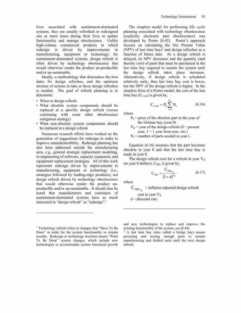
The simplest model for performing life cycle planning associated with technology obsolescence (explicitly electronic part obsolescence) was developed by Porter [6.45]. Porter’s approach focuses on calculating the Net Present Value (NPV) of last time buys2 and design refreshes as a function of future date. As a design refresh is delayed, its NPV decreases and the quantity (and thereby cost) of parts that must be purchased in the last time buy required to sustain the system until the design refresh takes place increases. Alternatively, if design refresh is scheduled relatively early, then last time buy cost is lower, but the NPV of the design refresh is higher. In the simplest form of a Porter model, the cost of the last time buy (CLTB) is given by,

∑=

=RY

0ii0LTB NPC (6.16)

where P0 = price of the obsolete part in the year of

the lifetime buy (year 0) YR = year of the design refresh (0 = present

year, 1 = 1 year from now, etc.) Ni = number of parts needed in year i.

Equation (6.16) assumes that the part becomes

obsolete in year 0 and that the last time buy is made in year 0.

The design refresh cost for a refresh in year YR (in year 0 dollars), CDR, is given by,

( ) R

RY

Y

DRIDR d1

CC

+= (6.17)

where

RYDRIC = inflation adjusted design refresh

cost in year YR d = discount rate.

and new technologies to replace and improve the existing functionality of the system, see [6.44]. 2 A last time buy (also called a bridge buy) means procuring and storing enough parts to sustain manufacturing and fielded units until the next design refresh.


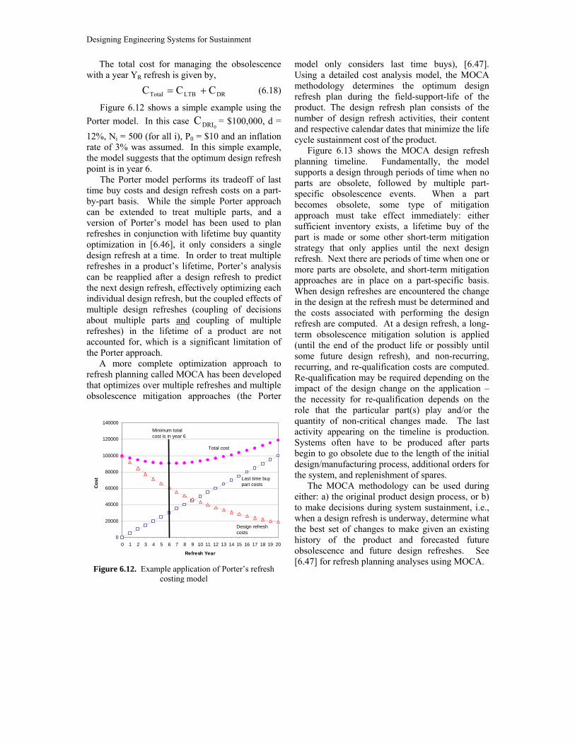
The total cost for managing the obsolescence with a year YR refresh is given by,

DR LTBTotal CCC += (6.18)

Figure 6.12 shows a simple example using the Porter model. In this case

0DRIC = $100,000, d = 12%, Ni = 500 (for all i), P0 = $10 and an inflation rate of 3% was assumed. In this simple example, the model suggests that the optimum design refresh point is in year 6.

The Porter model performs its tradeoff of last time buy costs and design refresh costs on a part-by-part basis. While the simple Porter approach can be extended to treat multiple parts, and a version of Porter’s model has been used to plan refreshes in conjunction with lifetime buy quantity optimization in [6.46], it only considers a single design refresh at a time. In order to treat multiple refreshes in a product’s lifetime, Porter’s analysis can be reapplied after a design refresh to predict the next design refresh, effectively optimizing each individual design refresh, but the coupled effects of multiple design refreshes (coupling of decisions about multiple parts and coupling of multiple refreshes) in the lifetime of a product are not accounted for, which is a significant limitation of the Porter approach.

A more complete optimization approach to refresh planning called MOCA has been developed that optimizes over multiple refreshes and multiple obsolescence mitigation approaches (the Porter

model only considers last time buys), [6.47]. Using a detailed cost analysis model, the MOCA methodology determines the optimum design refresh plan during the field-support-life of the product. The design refresh plan consists of the number of design refresh activities, their content and respective calendar dates that minimize the life cycle sustainment cost of the product.

Figure 6.13 shows the MOCA design refresh planning timeline. Fundamentally, the model supports a design through periods of time when no parts are obsolete, followed by multiple part-specific obsolescence events. When a part becomes obsolete, some type of mitigation approach must take effect immediately: either sufficient inventory exists, a lifetime buy of the part is made or some other short-term mitigation strategy that only applies until the next design refresh. Next there are periods of time when one or more parts are obsolete, and short-term mitigation approaches are in place on a part-specific basis. When design refreshes are encountered the change in the design at the refresh must be determined and the costs associated with performing the design refresh are computed. At a design refresh, a long-term obsolescence mitigation solution is applied (until the end of the product life or possibly until some future design refresh), and non-recurring, recurring, and re-qualification costs are computed. Re-qualification may be required depending on the impact of the design change on the application – the necessity for re-qualification depends on the role that the particular part(s) play and/or the quantity of non-critical changes made. The last activity appearing on the timeline is production. Systems often have to be produced after parts begin to go obsolete due to the length of the initial design/manufacturing process, additional orders for the system, and replenishment of spares.

The MOCA methodology can be used during either: a) the original product design process, or b) to make decisions during system sustainment, i.e., when a design refresh is underway, determine what the best set of changes to make given an existing history of the product and forecasted future obsolescence and future design refreshes. See [6.47] for refresh planning analyses using MOCA.

0

20000

40000

60000

80000

100000

120000

140000

0 1 2 3 4 5 6 7 8 9 10 11 12 13 14 15 16 17 18 19 20

Refresh Year

Cos

t

Last time buy part costs

Design refresh costs

Total cost

Minimum total cost is in year 6

Figure 6.12. Example application of Porter’s refresh costing model


Software Obsolescence [6.48]

In most complex systems, software life cycle costs contribute as much or more to the total life cycle cost as the hardware, and the hardware and software must be co-sustained. Software obso-lescence is usually caused by one of the following: 1. Functional Obsolescence: Hardware,

requirements, or other software changes to the system, obsolete the functionality of the software (includes hardware obsolescence precipitated software obsolescence; and software that obsoletes software).

2. Technological Obsolescence: The sales and/or support for COTS software terminates: • The original supplier no longer sells the

software as new • The inability to expand or renew licensing

agreements (legally unprocurable) • Software maintenance terminates - the

original supplier and third parties no longer support the software

3. Logistical Obsolescence: Digital media obsolescence, formatting, or degradation limits or terminates access to software. Analogously, hardware obsolescence can be

categorized similarly to software obsolescence: functional obsolescence in hardware is driven by software upgrades that will not execute correctly

on the hardware (e.g., Microsoft Office 2005 will not function on a 80486 processor based PC); technological obsolescence for hardware means that more technologically advanced hardware is available; and logistical obsolescence means that you can no longer procure a part.

Although some proactive measures can be taken to reduce the obsolescence mitigation footprint of software including: making code more portable, using open-source software, and third-party escrow where possible; these measures fall short of solving the problem and it is not practical to think that software obsolescence can somehow be avoided. Just like hardware, military and avionics systems have little or no control over the supply chain for COTS software or much of the software development infrastructure they may depend upon for developing and supporting organic software. Need proof? Consider the following quote from Bill Gates [6.49]: “The only big companies that succeed will be those that obsolete their own products before someone else does.” Obviously, Microsoft’s business plan is driven by motivations that do not include minimizing the sustainment footprint of military and avionics systems.

In the COTS world, hardware and software have developed a symbiotic supply chain relationship where hardware improvements drive software manufactures to obsolete software, which in turn cause older hardware to become obsolete –

Start of Life

Part becomes obsolete

Part is not obsolete Part is obsolete short term mitigation strategy used

Design refresh

• Spare replenishment• Other planned production

“Short term”mitigation strategy

• Existing stock• Last time buy• Aftermarket source

• Lifetime buy

“Long term” mitigation strategy

• Substitute part• Emulation• Uprate similar part

Redesign non-recurring costs

Re-qualification?• Number of parts changed• Individual part properties

Functionality Upgrades

Hardware and Software

Figure 6.13. Design refresh planning analysis timeline (presented for one part only, for simplicity, however in reality, there are coupled parallel timelines for many parts, and design refreshes and production events can occur

multiple times and in any order)


from Dell and Microsoft’s viewpoint, this is a win-win strategy. Besides COTS software (hardware specific and non-hardware specific), system sustainment depends on organic application software, software that provides infrastructure for hardware and software development and testing, and software that exists at the interfaces between system components (enabling interoperability. While hardware obsolescence precipitated software obsolescence is becoming primarily an exercise in finding new COTS software (and more often COTS software and new hardware are bundled together), the more challenging software obsolescence management problem is often found at the interfaces between applications, applications and the operating system, and drivers. One particular class of functional obsolescence of software that is becoming increasingly troublesome for many systems is security holes.

In reality, obsolescence management is a hardware/software co-sustainment problem, not just a hardware sustainment problem. Software obsolescence (and its connection to hardware obsolescence) is not well defined and current obsolescence management strategic planning tools are not generally capable of capturing the connection between hardware and software. For additional information on various aspects of software obsolescence, readers are encouraged to see [6.50,6.51]. 6.4 Technology Insertion

Each technology used in the implementation of

a system (i.e., hardware, software, the technologies used to manufacture and support the system,

information, and intellectual property) can be characterized by a life cycle that begins with introduction and maturing of the technology, and ends in some type of unavailability (obsolescence). The developers of sustainment-dominated systems must determine when to get off one technology’s life cycle curve and onto another’s in order to continue supporting existing systems and accommodate evolving system requirements, (Figure 6.14).

In order to manage the insertion of new technologies into a system, organizations need to maintain an understanding of technology evolution and maturity (“technology monitoring and forecasting”), measure the value of technology changes to their systems (“value metrics”), and build strategic plans for technology changes they wish to incorporate (“roadmapping”).

Technology Monitoring and Forecasting

Attempts to predict the future of technology and to characterize its affects have been undertaken by many different organizations, which use many different terms to describe their forward-looking actions. These terms include “technological intelligence”, “technology foresight”, “technology opportunities analysis (TOA)” [6.52], “competitive technological intelligence”, and “technology assessment” [6.53]. These terms fall under two, more general umbrella terms: ‘technology monitoring’ and ‘technology forecasting’. To monitor is “to watch, observe, check and keep up with developments, usually in a well-defined area of interest for a very specific purpose,” [6.54]. Technology monitoring is the process of observing

Time

Tech

nolo

gy C

ost

Technology Development

Technology Obsolescence

Extending technology availability is only possible if you have control over your supply chain

Time

Tech

nolo

gy C

ost When do you get off one

curve and on to the next?

Figure 6.14. Supporting systems and evolving requirements


new technology developments and following up on the developments that are relevant to an organization’s goals and objectives. Technology forecasting, like technology monitoring, takes stock of current technological developments, but takes the observation of technology a step further by projecting the future of these technologies and by developing plans for utilizing and accommodating them.

For high-volume consumer oriented products, there are many reasons for organizations to monitor and forecast technological advances. First, when the organization’s products are technologically-based, a good understanding of a nascent technology is needed as early as possible in order to take advantage of it. Additionally, monitoring and forecasting technology allows organizations to find applications for new technology [6.53], manage the technologies that are seen as threats, prioritize research and development, plan new product development, and make strategic decisions [6.55]. For manufacturers of sustainment-dominated products, monitoring and forecasting technology is of interest for the reasons listed above and also to enable prediction of obsolescence of the currently used technologies.

The primary method for locating and evaluating materials relevant to technology monitoring is a combination of text mining and bibliometric analysis. These methods monitor the amount of activity in databases on certain specified topics and categorize the information found into graphical groupings. Because of the amount of literature available on a given technology, much of the text mining process has been automated and computerized. Software is used to monitor databases of projects, research opportunities, publications, abstracts, citations, patents, and patent disclosures [6.55]. The general methodology for the automated text mining process is summarized in Figure 6.15.

The monitoring process involves identifying relevant literature by searching text that has been converted into numerical data [6.56]. Often there are previously defined search criteria and search bins where results can be placed. After literature has been found it must be clustered [6.57] with similar findings and categorized into trends. The

data is categorized using decision trees, decision rules, k-nearest neighbors, Bayesian approaches, neural networks, regression models and vector-based models [6.56]. This categorization allows hidden relationships and links between data sets to be determined, and helps locate gaps in the data, [6.57]. Once the data has been grouped, it is organized graphically in a scatter-plot form. Each point on the scatter plot can represent either a publication or an author. These points can be linked or grouped together to show the relationships and similarities between points.

The monitored data must then be interpreted and analyzed to determine which new technologies are viable and relevant. To do this, many organizations network with experts in related fields, and they employ surveys and other review techniques similar to the Delphi method [6.58] to force consensus among the experts. Expert opinion allows organizations to assess the implications of a new technology, and it is the first step in planning and taking action to cope with the benefits and risks associated with a new technology [6.52].

Technology monitoring and forecasting methods are still relatively new and untested, especially for larger databases of documents. Automated methods of forecasting and monitoring need to be refined and improved upon before they truly perform as they are intended to. Additionally, these tools will need to operate on a larger scale

1. Monitor Literature

2. Profile and Categorize Findings

3. Represent Information Graphically

4. Analyze and Interpret the Information

Figure 6.15. Steps in the technology monitoring process


and in a more diverse environment. Also, many organizations will begin to seek customer and client input when monitoring and forecasting. Finally, forecasts will eventually be evaluated against global, political, environmental, and social trends [6.53], placing them in a broader context, and expanding their uses beyond single organizations.

Value Metrics and Viability

Value is used to refer to the relative usefulness of an object, technology, process, or service. In the case of a system, value is the relative benefit of some or all of the following: acquiring, operating, sustaining, and disposing of the system. One way to represent value is shown in Figure 6.16, [6.59]. The “Attributes” axis includes measures of the application-specific direct product value. The “Conditions” axis includes details of the product usage and support environment. In simplified models, the Conditions axis provides the weights and constraints that govern how the Attributes are combined together. The “Time” axis is the “instantaneous time value”, i.e., value at a particular instant in time. Particular attributes may be weighted more than other attributes and their relative weightings are functions of time. For example, the value attributes during the final 20 seconds of a torpedo’s life are weighted differently than the value attributes during its prior 10 year storage life. All three axes in Figure 6.16 can be integrated. For example, if you integrate over the Time (instantaneous time value) axis, you get “sustainability value”. Integrating over the time axis tells you things about value attributes like “total cost of ownership” and availability. You could also integrate over the conditions axis, which would give you a measure how you are balancing multiple stakeholder’s conflicting requirements. Integration along the attributes axis builds composite value metrics.

A special case of Figure 6.16 is viability that addresses the application-specific impact of technology decisions on the life cycle of a system [6.60]. The objective of evaluating viability is to enable a holistic view of how the technology (and specific product) decisions made early in the

design process impact the life cycle affordability of a system solution.

We define viability as a monetary and non-monetary quantification of application-specific risks and benefits in a design/support environment that is highly uncertain. The definition of viability used in this discussion is a combination of economics and technical “value”, but assumes that technical feasibility has already been achieved. Traditional “value” metrics go part of the way toward defining viability by providing a coupled view of performance, reliability and acquisition cost, but are generally ignorant of how product sustainment may be impacted. We require a viability metric that measures both the value of the technology refreshment and insertion, and the degree to which the proposed change impacts the system’s current and future affordability and capability needs. This viability assessment must include hardware, software, information and intellectual property aspects of the product design. Viability therefore goes beyond just an assessment of the immediate, or near-term impacts of a technology insertion, in that it evaluates the candidate design (or candidate architecture) over its entire lifetime.

Although viability can be defined in many ways, its underlying premise is that economic well-being is inextricably linked to the sustainability of the system. According to studies conducted for the United States Air Force Engineering Directorate, [6.11]. Viability Assessment must include:

Conditions

Attributes

Time• Cost• Performance• Size• Reliability

• Stakeholders• Market conditions• Usage environment• Competition• Regulations

Figure 6.16. Three-dimensional value proposition [6.59]


• Producibility - Ability to produce the system in the future based upon the “current” architecture and design implementation. (production and initial spares, not replenishment spares).

• Supportability - Ability to sustain the system and meet the required operational capability rates. This includes repair and re-supply as well as non-recurring redesign for supportability of the “as is” design implementation and performance.

• Evolvability (Future Requirements Growth) - Ability of the system to support projected capability requirements with the “current” design. This includes capability implemented by hardware and software updates. The critical steps to making use of viability

concepts in decision making are: 1) Identifying practical and measurable indicators

of viability 2) Understanding how the indicators can be

measured as a function of decisions made (and time passed)

3) Managing the necessary qualitative and quantitative information (with associated uncertainty) needed to evaluate the indicators

4) Performing the evaluation (possibly linked to other analyses/tools that are used early in the design process). The viability of each technology decision made,

whether during the initial design of a product or during a redesign activity, should be evaluated. Viability is formulated from a mix of many things including the following two critical elements: • Technology life cycle – the life cycle of various

technology components (for example electronic parts) has been modeled and can be represented, e.g., technical life cycle maturity, lifecodes and obsolescence dates. The life cycle forecast may be dynamic and change (with time) in response to some form of technology surveillance program. In general, this metric is not application specific (and only hardware-part specific at this time). This concept, however, could be extended in two ways: 1) for a “technology group”, i.e., Computers, Memory, Bus Architectures, Sensors, Databases, Middleware, Operating Systems, etc. A “scaled-up” version of life cycle forecasting could

provide a maturity metric for a technology grouping versus a specific application that uses one (or a combination of) technology groups; and 2) for non-hardware components such as software, information and intellectual property.3 No present methodologies or tools are capable of assessing a particular technology category and mapping evolutions against the 30, 40 or 50 year life cycles that military systems and platforms are expected to perform.

• Associativity – the second element is the impact of a particular technology’s modification on the specific application. As an example, one technology may be late in its life cycle, but the impact of changing it on the application is low (making it a candidate for consideration), i.e., it is not in the critical path for qualification or certification, it does not precipitate any other changes to the application, or it is modularized in such a way as to isolate its impact on the rest of the system, i.e., a timing module that provides synchronization can be easily changed without impacting on any other part in the system and thus no associativity. On the other hand, other technologies (at the same point in their life cycle) may be central to everything (such as an Operating System or Bus Architecture) and therefore have high associativity.4

3 For example, electronic part obsolescence forecasting benefits from the commonality of parts in many systems, non-electronic part obsolescence cannot take advantage of this situation, and therefore, common commercial approaches that depend on subjective supply chain information will likely be less useful for general non-electronic and non-hardware obsolescence forecasting. 4 This is important as we begin to consider the Affordability of a Technology Refresh or Insertion. It is also important to identify the “Critical System Elements”; one way to do this is by using acquisition cost multiplied by the quantity needed in a system. But an operating system is relatively inexpensive and yet very critical. Thus the ‘value’ of the operating system is NOT just its acquisition cost multiplied by its quantity, but should also sum all of the acquisition costs (multiplied by quantities) of all effected parts of the system refreshment. This would be done for each element in the system Bill of Materials, and thus a new


When formulating the indicators of viability, the methodology must accommodate the fact that there are many stakeholders who all possess different portions of the knowledge necessary to accurately evaluate the viability of a specific choice or decision. Another difficulty is that the information necessary to make the decision is generally incomplete, and consists of qualitative and quantitative content and their associated uncertainties. Thus viability evaluation represents an information fusion problem.5 Roadmapping

Technology Roadmapping is a step in the strategic planning process that allows organizations to systematically compare the many paths toward a given goal or result while aiding in selecting the best path to that goal.

Many organizations have been forced to increase their focus on technology as the driver behind their product lines and business goals. This is different from the focus on customer wants and needs and the competitive demands that have previously determined the path of an industry. Technology roadmaps are seen as a way to combine customer needs, future technologies, and market demands in a way that is specific to the organization, and enables mapping a specific plan

sorting of the Bill of Materials would highlight the “System Critical Elements” by their impact to change. System Critical really refers to “Difficulty to Change based on Affordability”. This is also important because technology management represents a cost, and thus must focus on the system elements that drive cost. 5 Information fusion is the seamless integration of information from disparate sources that results in an entity that has more value (and less uncertainty) than the individual sources of information used to create it. Fused information is information that has been integrated across multiple data collection "platforms" (soft and hard) and physical boundaries, then blended thematically, so that the differences in resolution and coverage, treatment of a theme, character and artifacts of data collection methods are eliminated.

for technologies and the products and product lines they will affect.

Physically, the nodes and links depicted in roadmaps contain quantitative and qualitative information regarding how science, technology, and business will come together in a new or novel way to solve problems and reach the organization’s end goal, [6.61]. The time domain factors into the roadmap because it takes time for new technologies to be discovered, become mature, and be incorporated into a product, and for market share to grow to encompass new products, or for new possibilities to arise. In essence, technology roadmaps are graphical representations of the complex process of “identifying, selecting, and developing technology alternatives to satisfy a set of product needs,” [6.62].

It is important to note that, like their real world counterparts, technology roadmaps are not just needs driven documents (as in, “I need to get somewhere, what direction do I go?”) but can also be based on current position (as in, “Where could we go from here?”). It should also be stressed that roadmapping is an iterative process and that roadmaps must be continually maintained and kept up to date [6.63]. This is because the information contained in the roadmaps will change as time passes and new paths emerge or old paths disappear, and because an iterative roadmapping process will lead to a mature roadmap with clear requirements and fewer unknowns [6.64]. An iterative roadmapping process also leads to better understanding and standardization of the process, allowing roadmaps to be created more quickly, and the information in them to be more valuable.

Regardless of the type of roadmap and the information it contains, all roadmaps seek to answer three basic questions [6.64]:

1) Where are we going? 2) Where are we now? 3) How can we get there?

The process of creating a roadmap should answer these questions by listing and evaluating the possible paths to an end goal, and result in the selection of a single path to focus funding and resources on. Despite selecting a ‘final path’, companies should remain open minded and keep alternative paths open in case a poor decision has


been made. This is yet another reason to continually update the roadmap, since it serves as a mechanism to correct previous bad decisions.

Developing strategies and roadmaps that leverage technology evolution has been of interest for some time. The difficulty with historic roadmapping-based strategies is that they are: 1) inherently not application-specific and 2) tend to focus more on accurately forecasting the start of the technology life (when the technology becomes available and mature) and ignore the end of the technology life (obsolescence). While this roadmapping approach may be acceptable for those product sectors where there is no requirement for long-term sustainment (e.g., consumer electronics), it is not acceptable to sustainment-dominated product sectors. Thus the process of roadmapping will need to grow and develop if it is to be used by the sustainment industry. Since product roadmapping is still a relatively new process it will gradually become more application specific and more defined as time passes.

The design refresh planning tool discussed in Section 4, MOCA, has been extended to include technology roadmapping constraints, [6.65]. MOCA maps technology roadmap constraints into 1) timing constraints on its timeline, i.e., periods of time when one or more refreshes (redesigns) must take place in order to satisfy technology insertion requirements; 2) constraints on which parts or groups of parts must be addressed at certain refreshes (redesigns); and 3) additional costs for redesign activities.

6.5 Concluding Comments

Over the past 20 years, the use of the term

sustainability has been expanded and applied to the management of environmental, business, and technology issues. In the case of environmental and business, sustainability often refers to balancing or integration of issues [6.1], while for technology its meaning is much closer to the root definition meaning to maintain or continue.

For many systems the largest single expenditure is for operation and support. Sustainment of military equipment was recognized as early as the 6th century BC as a significant cost driver by Sun-

tzu in the Art of War [6.66]: “Government expenses for broken chariots, worn-out horses, breast-plates and helmets, bows and arrows, spears and shields, protective mantles, draught-oxen and heavy wagons, will amount to four-tenths of its total revenue.” Today it’s not just military systems but many other systems ranging from avionics to traffic lights and the technology content in rides at amusement parks.

Failure to proactively sustaining the technological content of systems is no longer an option for many types of systems. System evolution is not free and also cannot be avoided, proactive solutions are required in order to maintain market share and/or affordably provide continued system support and operation. References [6.1] Sutton, P., “What is Sustainability?”

Eingana, Vol. 27, No. 1, Apr 2004, pp. 4-9.

[6.2] Costanza, R., Ecological Economics: The Science and Management of Sustainability, Columbia University Press, 1991.

[6.3] Brundtland Commission, Our common future. World Commission on Environment and Development, 1987.

[6.4] ForestERA, http://www.forestera.nau.edu/glossary.htm

[6.5] Elkington, J., Cannibals with Forks: The Triple Bottom Line of 21st Century Business, Capstone Publishing Ltd, 1997.

[6.6] Kleindorfer, P.R., Singhal, K., and Van Wassenhove, L.N., “Sustainable Operations Management,” Production and Operations Management, Vol. 14, No. 4, Winter 2005, pp. 482-492.

[6.7] Crum, D., “Legacy System Sustainment Engineering,” Proceedings of the Diminishing Manufacturing Sources and Material Shortages Conference, New Orleans, LA, March 2002. available at: http://smaplab.ri.uah.edu/dmsms02/presentations/crum.pdf


[6.8] Cost Analysis Improve. Group (CAIG), “Operating and Support Cost-Estimating Guide,” Office of the Sec. of Defense, http://www.dtic.mil/pae/, May 1992

[6.9] Gateway Inc., www.gateway.com, December 2001.

[6.10] Shields, P., “Total Cost of Ownership: Why the price of the computer means so little”, http://www.thebusinessmac.com/ features/tco_hardware.shtml, December 2001.

[6.11] Ardis, B., “Viable/Affordable Combat Avionics (VCA) Implementation Update,” Dayton Aerospace, Inc., June 2001.

[6.12] “Reliability and Support Factors,” http://home.wanadoo.nl/jdonders/AVAIL.html

[6.13] Myrick, A., “Sparing Analysis – A Multi-Use Planning Tool,” Proceedings of the Reliability and Maintainability Symposium, pp. 296-300, 1989.

[6.14] McDougall, R., “Availability – What I Means, Why It’s Important, and How to Improve It,” Sun BluePrints OnLine, Oct. 1999, http://www.sun.com/blueprints/1099/ availability.pdf

[6.15] “Performance Based Logistics: A Program Manager’s Product Support Guide,” Defense Acquisition University Press, March 2005, http://www.dau.mil/ pubs/misc/PBL_Guide.pdf

[6.16] Lie, C.H., Hwang, C.L., and Tillman, F.A., “Availability of Maintained Systems: A State-of-the-Art Survey,” AIIE Trans., Vol. 9, No. 3, 1977, pp. 247-259.

[6.17] “LM-720 Reliability, Availability, & Maintainability (RAM) (Hardware and Software),” https://acc.dau.mil/getattachment.aspx?id=22523&pname=file&aid=2212

[6.18] Coughlin, R.J., “Optimization of Spares in a Maintenance Scenario,” Proceedings of

the Reliability and Maintainability Symposium, 1984, pp. 371-376.

[6.19] Adams, C.M., “Inventory Optimization Techniques, System vs. Item Level Inventory Analysis,” Proceedings of the Reliability and Maintainability Symposium, 2004, pp. 55-60.

[6.20] Sherbrooke, C.C., Optimal Inventory Modeling of Systems: Multi-Echelon Techniques, Wiley, New York, NY, 1992.

[6.21] Murthy, D.N.P. and Djamaludin, I., “New Product Warranty: A Literature Review,” Int. Journal of Production Economics, Vol. 79, No. 3, 2002, pp. 231-260.

[6.22] Elsayed, E.A., Reliability Engineering, Addison Wesley, 1996.

[6.23] Blischke, W.R. and Murthy, D.N.P., Warranty Cost Analysis, Marcel Dkker, 1994.

[6.24] Hunter, J.J., “Mathematical Techniques for Warranty Analysis,” Product Warranty Handbook, ed. W.R. Blishke and D.N.P. Murthy, New York, Marcel Dekker, 1996.

[6.25] Feldman, K. and Sandborn, P., “Integrating Technology Obsolescence Considerations into Product Design Planning,” Proceedings of the ASME Design for Manufacturing and Life Cycle Conference, Las Vegas, NV, September 2007.

[6.26] QTEC, http://www.qtec.us/Products/QStar_Introduction.htm, 2006.

[6.27] Masters, J.M., “A Note on the Effect of Sudden Obsolescence on the Optimal Lot Size,” Decision Sciences, Vol. 22, No. 5, Nov/Dec 1991, pp. 1180-1186.

[6.28] Perry, W. (1994), U.S. Secretary of Defense.

[6.29] Henke, A.L. and Lai, S., “Automated Parts Obsolescence Prediction,” Proceedings of the DMSMS Conference, 1997.


[6.30] Josias, C., Terpenny, J.P., and McLean K.J., “Component Obsolescence Risk Assessment,” Proceedings of the 2004 Industrial Engineering Research Conference (IERC), 2004.

[6.31] Solomon, R., Sandborn, P., and Pecht, M., “Electronic part life cycle concepts and obsolescence forecasting,” IEEE Trans. on Components and Packaging Technologies, Vol. 23, December 2000, pp. 707-713.

[6.32] Meixell, M. and Wu, S.D., “Scenario analysis of demand in a technology market using leading indicators,” IEEE Trans. on Semi. Manuf., Vol. 14, 2001, pp. 65-78.

[6.33] Sandborn, P., Mauro, F., and Knox, R., “A data mining based approach to electronic part obsolescence forecasting,” to be published IEEE Trans. on Components and Manufacturing Technology.

[6.34] Tilton, J.R., “Obsolescence Management Information System (OMIS),” http://www.jdmag.wpafb.af.mil/elect%20obsol%20mgt.pdf, NSWC Keyport

[6.35] Howard, M.A., “Component Obsolescence – It’s Not Just for Electronics Anymore. Proceedings of the Aging Aircraft Conference, 2002.

[6.36] ARINC, Inc., ARINC Logistics Assessment and Risk Management (ALARM) Tool, http://www.arinc.com/ news/2005/06-28-05.html

[6.37] Stogdill, R.C., “Dealing with Obsolete Parts,” IEEE Design & Test of Computers, Vol. 16, 1999, pp. 17-25.

[6.38] Pecht, M. and Tiku, S., “Electronic Manufacturing and Consumers Confront a Rising Tide of Counterfeit Electronics,” IEEE Spectrum, Vol. 43, No. 5, May 2006, pp. 37-46.

[6.39] Johnson, W., “Generalized Emulation of Microcircuits,” Proceedings of the DMSMS Conference, 2000.

[6.40] Pecht, M. and Humphrey, D., “Uprating of

Electronic Parts to Address Obsolescence,” Microelectronics International, Vol. 23, No. 2, 2006, pp. 32-36.

[6.41] Feng, D., Singh, P., and Sandborn, P., “Optimizating Lifetime Buys to Minimize Lifecycle Cost,” Proceedings of the Aging Aircraft Conference, Palm Springs, CA, April 2007.

[6.42] Sandborn, P., “Beyond Reactive Thinking – We Should be Developing Pro-Active Approaches to Obsolescence Management Too!” DMSMS COE Newsletter, Vol. 2, Issue 3, 2004, pp. 4 and 9.

[6.43] Robbins, R.M., “Proactive Component Obsolescence Management,” A-B Journal, Vol. 10, 2003, pp. 49-54.

[6.44] Herald, T.E., “Technology Refreshment Strategy and Plan for Application in Military Systems – A How-To Systems Development Process and Linkage with CAIV,” Proc. National Aerospace and Electronics Conference (NAECON), October 2000, pp. 729-736.

[6.45] Porter, G.Z., “An Economic Method for Evaluating Electronic Component Obsolescence Solutions,” Boeing Company White Paper, 1998.

[6.46] Cattani, K.D. and Souza, G.C., “Good buy? Delaying End-of-Life Purchases.” European J. of Operational Research, Vol. 146, 2003, pp. 216-228.

[6.47] Singh, P. and Sandborn, P., "Obsolescence Driven Design Refresh Planning for Sustainment-Dominated Systems," The Engineering Economist, Vol. 51, No. 2, April-June 2006, pp. 115-139.

[6.48] Sandborn, P. and Plunkett, G., “The Other Half of the DMSMS Problem - Software Obsolescence,” DMSMS Knowledge Sharing Portal Newsletter, Vol. 4, Issue 4, June 2006, pp. 3 and 11.

[6.49] Gates, B., Founder, Chairman, Microsoft Corp. “The Bill Gates Method,” APT News, July 21, 2003.


[6.50] Merola, L., “The COTS Software Obsolescence Threat,” Proceedings of the International Conference on Commercial-Off-The-Shelf (COTS) Based Software Systems, 2006.

[6.51] Rickman, T. and Singh, G., “Strategies for Handling Obsolescence, End-of-Life and Long-Term Support of COTS Software,” COTS Journal, January 2002, pp. 17-21.

[6.52] Porter, A.L., Jin, X.-Y., et al., “Technology Opportunities Analysis: Integrating Technology Monitoring, Forecasting, and Assessment with Strategic Planning,” SRA J., Vol. 26, No. 2, Oct. 1, 1994, pp. 21-31.

[6.53] Coates, V., Faroque, M., Klavins, R., Lapid, K., Linstone, H.A., Pistorius, C., and Porter, A.L., “On the Future of Technological Forecasting,” Technology Forecasting and Social Change, Vol. 67, No. 1, 2001, pp. 1–17.

[6.54] Porter, A.L. and Detampel, M.J., “Technology Opportunities Analysis,” Tech. Forecasting and Social Change, Vol. 49, No. 3, July 1995, pp. 237-255.

[6.55] Zhu, D. and Porter, A.L., “Automated extraction and visualization of information for technological intelligence and forecasting,” Technological Forecasting and Social Change, Vol. 69, Issue 5, June 2002, pp. 495-506.

[6.56] Teichert, T. and Mittermayer, M.A., "Text Mining for Technology Monitoring," Proceedings of the IEEE International Engineering Management Conference (IEMC), Vol. 2, 2002, pp. 596- 601.

[6.57] Zhu, D., Porter, A., et al., “A Process for Mining Science & Technology Documents Databases, Illustrated for the Case of ‘Knowledge Discovery and Data Mining’. Cienc Inf., Vol. 28, No. 1, 1999, pp. 1-8.

[6.58] Helmer, O., “Analysis of the Future: The Delphi Method;” and “The Delphi Method: An Illustration,” Technological Forecasting for Industry and Government, Bright, J. Ed.

Prentice Hall, Englewood Cliffs, NJ, 1968.

[6.59] Nassar, A., “Product Value Proposition: A Step by Step Approach,” Intercontinental Networks White Paper, April 2003, http://www.anassar.net.

[6.60] Sandborn, P., Herald, T., Houston, J., and Singh, P., “Optimum Technology Insertion into Systems Based on the Assessment of Viability. IEEE Trans. on Comp. and Pack. Tech, Vol. 26, 2003, pp. 734-738.

[6.61] Kostoff, R.N. and Schaller, R.R., “Science and Technology Roadmaps,” IEEE Trans. on Engineering Management, Vol. 48, No. 2, 2001, pp. 132–143.

[6.62] Walsh, S.T., “Roadmapping a Disruptive Technology: A Case Study: The Emerging Microsystems and Top-Down Nanosystems Industry,” Technological Forecasting and Social Change, Vol. 71, Nos. 1-2, January-February 2004, pp. 161-175.

[6.63] Rinne, M., “Technology Roadmaps: Infrastructure for Innovation,” Tech. Forecasting & Social Change, Vol. 71, Nos. 1-2, 2004, pp. 67-80.

[6.64] Phaal, R., Farrukh, C., and Probert, D., “Developing a Technology Roadmapping System,” Technology Management: A Unifying Discipline for Malting the Boundaries, T.R. Anderson, D.F. Kocaoglu, and T.U. Daim, Eds. Portland: PICMET, 2005.

[6.65] Myers, J. and Sandborn, P., “Integration of Technology Roadmapping Information and Business Case Development into DMSMS-Driven Design Refresh Planning of the V-22 Advanced Mission Computer,” Proceedings of the Aging Aircraft Conference, Palm Springs, CA, April 2007.

[6.66] Sun-tzu, The Art of War, Translated by R.D. Sawyer, MetroBooks, New York, NY, March 2002.