548 63 final report-1-29-10

_______________________________________ FINAL REPORT U.F. Project No. 00054863 RPWO#: 60 Contract No: BD545

_______________________________________ DEVELOPMENT OF DESIGN PARAMETERS

FOR MASS CONCRETE USING FINITE

ELEMENT ANALYSIS

_______________________________________ Mang Tia Christopher Ferraro Adrian Lawrence Samuel Smith

Eiji Ochiai

_______________________________________ February 2010

Department of Civil & Coastal Engineering College of Engineering University of Florida Gainesville, Florida 32611

_______________________________________

ii

DISCLAIMER

“The opinions, findings, and conclusions expressed

inthis publication are those of the authors and not

necessarily those of the State of Florida Department

of Transportation or the U.S. Department of

Transportation.

Prepared in cooperation with the State of Florida

Department of Transportation and the U.S. Depart-

ment of Transportation.”

iii

SI (MODERN METRIC) CONVERSION FACTORS (from FHWA)

APPROXIMATE CONVERSIONS TO SI UNITS

SYMBOL WHEN YOU KNOW MULTIPLY BY TO FIND SYMBOL

LENGTH

in inches 25.4 millimeters mm

ft feet 0.305 meters m

yd yards 0.914 meters m

mi miles 1.61 kilometers km


AREA

in2 squareinches 645.2 square millimeters mm2

ft2 squarefeet 0.093 square meters m2

yd2 square yard 0.836 square meters m2

ac acres 0.405 hectares ha

mi2 square miles 2.59 square kilometers km2


VOLUME

fl oz fluid ounces 29.57 milliliters mL

gal gallons 3.785 liters L

ft3 cubic feet 0.028 cubic meters m3

yd3 cubic yards 0.765 cubic meters m3

NOTE: volumes greater than 1000 L shall be shown in m3


MASS

oz ounces 28.35 grams g

lb pounds 0.454 kilograms kg

T short tons (2000 lb) 0.907 megagrams (or "metric ton")

Mg (or "t")


TEMPERATURE (exact degrees) oF Fahrenheit 5 (F-32)/9

or (F-32)/1.8 Celsius oC


ILLUMINATION

fc foot-candles 10.76 lux lx

fl foot-Lamberts 3.426 candela/m2 cd/m2


FORCE and PRESSURE or STRESS

lbf poundforce 4.45 newtons N

lbf/in2 poundforce per square inch 6.89 kilopascals kPa

iv

APPROXIMATE CONVERSIONS TO SI UNITS


LENGTH

mm millimeters 0.039 inches in

m meters 3.28 feet ft

m meters 1.09 yards yd

km kilometers 0.621 miles mi


AREA

mm2 square millimeters 0.0016 square inches in2

m2 square meters 10.764 square feet ft2

m2 square meters 1.195 square yards yd2

ha hectares 2.47 acres ac

km2 square kilometers 0.386 square miles mi2


VOLUME

mL milliliters 0.034 fluid ounces fl oz

L liters 0.264 gallons gal

m3 cubic meters 35.314 cubic feet ft3

m3 cubic meters 1.307 cubic yards yd3


MASS

g grams 0.035 ounces oz

kg kilograms 2.202 pounds lb

Mg (or "t") megagrams (or "metric ton") 1.103 short tons (2000 lb) T


TEMPERATURE (exact degrees) oC Celsius 1.8C+32 Fahrenheit oF


ILLUMINATION

lx lux 0.0929 foot-candles fc

cd/m2 candela/m2 0.2919 foot-Lamberts fl


FORCE and PRESSURE or STRESS

N newtons 0.225 poundforce lbf

kPa kilopascals 0.145 poundforce per square inch

lbf/in2

*SI is the symbol for International System of Units. Appropriate rounding should be made to comply with Section 4 of

ASTM E380.

(Revised March 2003)

v

TECHNICAL REPORT DOCUMENTATION PAGE 1. Report No.

000548 63 2. Government Accession No.

3. Recipient's Catalog No.

5. Report Date

February 2010 4. Title and Subtitle

Development of Design Parameters for Mass Concrete

Using Finite Element Analysis 6. Performing Organization Code

7. Author(s)

Mang Tia, Christopher Ferraro, Adrian Lawrence, Samuel Smith, and Fiji Ochiai

8. Performing Organization Report No.

000548 63

10. Work Unit No. (TRAIS)

9. Performing Organization Name and Address

Department of Civil and Coastal Engineering 365 Weil Hall – P.O. Box 116580 University of Florida Gainesville, FL 32611-6580

11. Contract or Grant No.

BD-545 #60

13. Type of Report and Period Covered

Final Report 11/10/05 - 12/15/09

12. Sponsoring Agency Name and Address

Florida Department of Transportation 605 Suwannee Street, MS 30 Tallahassee, FL 32399 14. Sponsoring Agency Code

15. Supplementary Notes

Prepared in cooperation with the U.S. Department of Transportation and the Federal Highway Administration

16. Abstract

A finite element model for analysis of mass concrete was developed in this study. To validate the developed model, large concrete blocks made with four different mixes of concrete, typical of use in mass concrete applica-tions in Florida, were made and monitored for their temperature and strain developments, and compared with the computed temperature and stress distributions from the finite element model. A parametric analysis was also conducted to determine the effects of various factors on the temperature distribution, induced stresses and the cracking risk. Investigation was also made on testing methods to measure the thermal and mechanical properties of mass concrete needed as input parameters for the finite element model. The findings from this study are as follows: (1) Results from the isothermal calorimetry test should be used for input for the heat generation function in the finite element modeling of concrete hydration; (2) Reliance on a limiting maximum temperature differential to control cracking in massive concrete applications should be supplemented with a suitable analysis to show that expected stresses will not exceed the strength of the concrete; (3) Adequate insulation should be used in conjunction with the usual formwork material to reduce the temperature differentials during the early age hydration of massive concrete; (4) A safety factor should be applied to the tensile strength values for concrete to guard against the initiation of micro-cracks; and (5) The current restrictions on maximum temperature imposed by state regulating bodies should take into consideration the type of cementitious materials that will be used in the concrete mix. 17. Key Words

Mass Concrete, Finite Element Model, Isothermal Calorimetry, Heat of Hydration, Insulation, Temperature Differential, Cracking Risk, Micro-cracks, Parametric Study, Tensile Strength.

18. Distribution Statement

No restrictions.

19. Security Classif. (of this report)

Unclassified 20. Security Classif. (of this page)

Unclassified 21. No. of Pages

194 22. Price

Form DOT F 1700.7 (8-72) Reproduction of completed page authorized

vi

ACKNOWLEDGMENTS

The Florida Department of Transportation (FDOT) is gratefully acknowledged for

providing the financial support for this study. The FDOT Materials Office provided the

additional testing equipment, materials, and personnel needed for this investigation. Sincere

thanks go to the project manager, Mr. Michael Bergin, for providing his technical coordination

and advice throughout the project. Sincere gratitude is extended to the FDOT Materials Office

personnel, particularly to Messrs. Charles Ishee, Mario Paredes, Richard DeLorenzo, Craig

Roberts, Joseph Fitzgerald, Toby Dillow, Luke Goolsby, Steven Sauls, Fred Yon, Alfred Camps,

Duane Robertson, Rahman Henderson, Dr. H. Deford, Ms. Susan Blazo, and Ms.Teresa Risher

for their invaluable help in this study. Sincere thanks also go to the support of the staff and

students at the Department of Civil and Coastal Engineering at the University of Florida,

particularly to Messrs. Chuck Broward, Tony Murphy, Hubert Martin, Boris Haranki, Patrick

Bekoe, Christopher Egan, James Falls, Gustavo Morris, and Ms. Carrie Ulm for their technical

support in the lab. Special thanks are due to Ms. Candace Leggett for her expert editing of this

report.

vii

EXECUTIVE SUMMARY

Background and Research Needs

Mass concrete is defined by the American Concrete Institute (ACI) as “any volume of

concrete with dimensions large enough to require that measures be taken to cope with generation

of heat from hydration of the cement and attendant volume change, to minimize cracking.” The

requirements for the control of heat generation and temperature distribution in mass concrete

vary on a state-by-state basis. Currently, there is no uniformity on the specifications on mass

concrete among the different state department of transportations in the United States. There is a

need to have an effective tool which can be used to accurately determine the temperature and

stress development in mass concrete elements and the conditions at which cracking may develop,

so that mass concrete can be properly specified, controlled, and produced with minimum

problems in service.

Research Objectives

The goal of this study is to develop a finite element model of mass concrete, which can

predict the temperature distribution during hydration and the thermal stresses that result from the

thermal gradients within the structure. Previous attempts at predicting the temperature distri-

bution in mass concrete by way of finite element models has mainly focused on using generic

heat generation functions for the calculation of adiabatic temperature rise. The heat generated by

hydrating mass concrete has also been widely modeled as being uniform throughout the concrete

mass, whereas in reality the heat generation is a function of the temperature and time history of

individual locations in the concrete mass. The developed finite element model will use accurate-

ly measured thermal and mechanical properties as input parameters, and will take into considera-

viii

tion the time-temperature conditions of individual locations within a hydrating mass concrete

structure. A stress analysis utilizing changing strength properties of the concrete will also be

conducted and the results compared with the experimental observation as a means of validation.

Another main objective of this study is to develop a test regimen and analysis methodology

to provide these necessary input parameters for the finite element model.

Research Approach

The modeling of a mass concrete element is done with the aid of the commercially

available TNO DIANA software. The analysis is done in two parts, firstly, a thermal analysis in

which the thermal properties are modeled, the hydration process simulated, and the resulting

temperature distribution obtained. The second part of the analysis is a stress analysis in which

the physical properties such as elastic modulus and coefficient of thermal expansion are used

along with the temperature histories obtained in the thermal analysis to calculate the stresses and

strains produced by the thermal gradients. The cracking potential is then assessed.

As a means of validation, four different mixes of concrete, typical of use in mass concrete

applications in Florida, were produced and each mix used to make two 3.5-ft. 3.5-ft. 3.5-ft.

concrete blocks. For each mix, one block was insulated on all six sides to simulate a fully

adiabatic process, while the other block was insulated on five of the faces with the top face left

open and exposed to environmental conditions. Measurements of the temperature and strain at

predetermined locations within the blocks were recorded until the equilibrium temperature was

achieved.

At the time of casting the blocks, concrete was taken from the same mix and evaluated for

mechanical properties at different ages, as well as thermal properties, heat of hydration, specific

heat capacity, and thermal diffusivity, which were then used as input to the finite element model.

ix

Finally, a parametric analysis was conducted to determine what effects the size of the

concrete structure, amount of insulation used, specific heat capacity, and diffusivity would have

on the temperature distribution, induced stresses, and the cracking risk.

Separate physical and thermal testing programs were also conducted to investigate state-of-

the-art testing methods and to determine those methods which are suitable as input parameters

for analysis of the behavior of mass concrete.

Findings

The two types of tests done on the concrete mixtures to determine the energy released

during hydration were semi-adiabatic calorimetry and isothermal calorimetry. The calculated

adiabatic energy rise obtained from each test was used in the model to determine which

procedure would give the best results when compared with the temperatures measured in the

experimental block.

Based on the results of the thermal analysis of the concrete block model, the following

findings were made:

The semi-adiabatic calorimetry test consistently gave lower heat of hydration and

lower predicted temperature of concrete as compared with the isothermal calorimetry

test.

The input of adiabatic energy captured in the isothermal calorimetry test provided

temperature distributions that were very similar to those measured in the experimental

blocks. At some locations, the predicted temperatures were higher than the measured

temperatures, and so the isothermal test can be said to provide conservative predictions

of the temperature distribution.

The induced stresses caused by the varying temperatures within the concrete element of

each mixture were analyzed using the results from the model that utilized the energy from the

x

isothermal calorimetry test. The results of this structural analysis for the concrete block study

led to the following observations:

The highest tensile stresses were located at the top edge of the surface exposed to

ambient conditions.

Concrete containing 100% Portland cement experienced tensile stresses high enough to

cause cracking on all surfaces, even those insulated, when the temperature difference

was 17.3°C (31.1° F).

In the case where 50% of the Portland cement was replaced with ground granulated

blast-furnace slag, the rate of hydration reaction, and hence, rate of temperature

increase was significantly slower. The associated reduction in early age tensile

strength resulted in the cracking risk not being reduced.

In the case where 35% of the Portland cement was substituted with fly ash, there was

little effect on the early age rate of hydration, and thus, the time in which the maximum

temperature was achieved was not affected significantly. However, the maximum

temperature achieved was itself significantly less. Again, the early age tensile strength

was less than the 100% Portland cement case, resulting in similar cracking on all

surfaces as before, even though the tensile stresses experienced were less.

Concrete that had a blend of 50% Portland cement, 30% slag, and 20% fly ash

performed the best in terms of reducing the induced thermal stresses relative to the

tensile strength, and hence, the cracking potential.

The temperature differential that induced cracking in the concretes used in this project

varied from mixture to mixture. This was due to the corresponding changes in the

tensile strength.

The parametric study on factors affecting the temperature distribution in concrete produced

the following results:

The thermal stresses in large mass concrete elements were effectively reduced with the

use of thick layers of insulating polystyrene foam. This method is advantageous

because the polystyrene foam, if removed carefully, can be reused, often making it

xi

relatively inexpensive when compared to other single-use methods such as cooling

pipes and liquid nitrogen.

Although the tensile stresses that resulted from the removal of formwork and insulation

12 hours, 1 day, 2 days, and 3 days after the pouring concrete were less than the tensile

strength of the concrete as measured in the laboratory, the stresses could be large

enough to initiate micro-cracking. These micro-cracks can serve as an entry point for

deleterious materials that can undermine the durability of the concrete. For insulation

removed after 4 days, the tensile stresses were significantly less than the tensile

strength, reducing the risk of micro-cracking.

Conclusions

Based on the results obtained in this study, the following conclusions are made:

The heat of hydration energy data obtained from the isothermal calorimetry test should

be used as the input for the heat generation function in the finite element modeling of

concrete hydration.

Reliance on a limiting maximum temperature differential to control cracking in

massive concrete applications should be supplemented with a requirement for the

presentation of a finite element analysis showing the calculated stress response to the

predicted temperature distribution within the concrete, to ensure that the induced

tensile stresses will not exceed the tensile strength of the concrete.

Adequate insulation should be used in conjunction with the usual formwork material to

reduce the temperature differentials during the early age hydration of massive concrete.

However, caution should be taken, as the occurrence of delayed ettringite formation

(DEF) and drying shrinkage due to high concrete temperatures was not studied.

A safety factor should be applied to the tensile strength values for concrete obtained

from the splitting tension and third-point flexural strength tests to guard against the

initiation of micro-cracks which, although by themselves, will not cause structural

failure, can act as an entry point for deleterious materials which can undermine the

durability of the concrete.

xii

The current restrictions on maximum temperature imposed by state regulating bodies

should take into consideration the type of cementitious materials that will be used in

the concrete mix.

Recommendations for Future Research

It is recommended that additional blends of cementitious materials and additional large

blocks of mass concrete be tested in order to assess the universal applicability of the hypotheses

deduced and concluded from this study.

xiii

TABLE OF CONTENTS page ACKNOWLEDGMENTS ............................................................................................................vi EXECUTIVE SUMMARY .........................................................................................................vii LIST OF TABLES......................................................................................................................xvi LIST OF FIGURES ...................................................................................................................xvii CHAPTER 1 INTRODUCTION ....................................................................................................... 1 1.1 Background......................................................................................................... 1 1.2 Present Specifications on Mass Concrete ........................................................... 3 1.3 Research Needs................................................................................................... 4 1.4 Objective of Study .............................................................................................. 5 1.5 Research Approach ............................................................................................. 6 1.6 Outline of Report ................................................................................................ 8 2 LITERATURE REVIEW ............................................................................................ 9 2.1 Introduction......................................................................................................... 9 2.2 Tensile Stresses in Mass Concrete.................................................................... 13 2.2.1 Tensile Stresses Due to Thermal Gradients .......................................... 13 2.2.2 Tensile Stresses Due to Delayed Ettringite Formation ......................... 17 2.3 Supplementary Cementitious Materials............................................................ 22 2.4 Long Spruce Dam Rehabilitation Project ......................................................... 23 2.5 Reinforced Concrete Wall on Basemat Concrete Slab Project ......................... 27 2.6 The James Bay Concrete Monolith Project ...................................................... 30 3 FINITE ELEMENT THERMAL MODEL................................................................ 34 3.1 Introduction....................................................................................................... 34 3.2 Element Selection ............................................................................................. 35 3.3 Input Parameters ............................................................................................... 37 3.3.1 Heat of Hydration ................................................................................. 37 3.3.2 Conductivity and Heat Capacity ........................................................... 42 3.3.3 Convection ............................................................................................ 44 3.4 Model Geometry ............................................................................................... 46 3.5 Boundary Conditions ........................................................................................ 46 4 FINITE ELEMENT STRUCTURAL MODEL......................................................... 49 4.1 Introduction....................................................................................................... 49 4.2 Element Selection ............................................................................................. 49 4.3 Material Model.................................................................................................. 50

xiv

4.4 Input Parameters ............................................................................................... 50 4.4.1 Modulus of Elasticity............................................................................ 50 4.4.2 Poisson’s Ratio...................................................................................... 51 4.4.3 Coefficient of Thermal Expansion........................................................ 51 4.4.4 Tensile Strength .................................................................................... 52 4.5 Symmetry and Boundary Conditions................................................................ 52 5 BLOCK EXPERIMENT ........................................................................................... 53 5.1 Introduction....................................................................................................... 53 5.2 Concrete Mix Design ........................................................................................ 53 5.3 Block Geometry ................................................................................................ 53 5.4 Instrumentation for Data Collection ................................................................. 55 5.5 Temperature Profiles......................................................................................... 55 6 MATERIAL TESTS AND PROPERTIES................................................................ 62 6.1 Introduction....................................................................................................... 62 6.2 Heat of Hydration ............................................................................................. 62 6.2.1 Semi-Adiabatic Calorimetry ................................................................. 62 6.2.2 Isothermal Conduction Calorimetry ..................................................... 63 6.3 Specific Heat Capacity...................................................................................... 66 6.4 Thermal Diffusivity .......................................................................................... 67 6.5 Flexural Strength............................................................................................... 69 6.6 Splitting Tensile Strength ................................................................................. 71 6.7 Modulus of Elasticity and Poisson’s Ratio Testing .......................................... 73 6.8 Coefficient of Thermal Expansion Testing....................................................... 74 6.9 Summary of Material Properties....................................................................... 75 7 THERMAL ANALYSIS RESULTS ......................................................................... 78 7.1 Introduction....................................................................................................... 78 7.2 Semi-Adiabatic Calorimetry Finite Element Results........................................ 81 7.3 Isothermal Calorimetry Finite Element Results................................................ 88 7.4 Summary of Findings........................................................................................ 96 8 STRUCTURAL ANALYSIS RESULTS .................................................................. 99 8.1 Stress Results .................................................................................................... 99 8.2 Cracking Potential........................................................................................... 105 8.3 Temperature Difference and Cracking............................................................ 109 8.4 Summary of Findings...................................................................................... 114 9 PARAMETRIC STUDY ......................................................................................... 115 9.1 Introduction..................................................................................................... 115 9.2 Effect of Specimen Size.................................................................................. 115 9.3 Effect of Insulation Thickness ........................................................................ 120 9.4 Time of Formwork Removal Effect................................................................ 128 9.5 Heat Generation Rate Effect ........................................................................... 134 9.6 Summary of Findings...................................................................................... 135

xv

10 RECOMMENDED TESTING REGIMEN FOR MASS CONCRETE................... 136 10.1 Recommended Testing Method for Measurement of Heat Generation .......... 136 10.2 Recommended Testing Method for Measuring Maturity/Equivalent Age ..... 137 10.3 Recommended Testing Methods for Strength and Modulus of Elasticity...... 138 10.3.1 Compressive Strength ......................................................................... 138 10.3.2 Compressive Modulus of Elasticity .................................................... 138 10.3.3 Tensile Strength ................................................................................. 139 10.4 Recommended Testing Method for Measurement of Coefficient

of Thermal Expansion..................................................................................... 139 10.5 Recommended Physical Parameter for the Concrete Diffusivity ................... 140 10.6 Recommended Physical Parameter for the Specific Heat Capacity ............... 140 10.7 Summary of Testing Program......................................................................... 141 11 CONCLUSIONS AND RECOMMENDATIONS .................................................. 142 11.1 Findings........................................................................................................... 142 11.2 Conclusions..................................................................................................... 144 11.3 Recommendations for Future Research .......................................................... 145 LIST OF REFERENCES........................................................................................................... 146 APPENDIX A GRAPHICAL USER INTERFACE INPUT COMMANDS ...................................A-1 B BATCH FILE INPUT COMMANDS .....................................................................B-1 C STAGGERED ANALYSIS COMMANDS ............................................................C-1 D PHASED ANALYSIS COMMANDS.....................................................................D-1 E METHOD OF TESTING FOR MEASURING THE HEAT

OF HYDRATION OF HYDRAULIC CEMENT USING ISOTHERMAL CONDUCTIVE CALORIMETRY............................................... E-1

xvi

LIST OF TABLES Table page 2-1 Cementitious Material Content for Concrete Materials .............................................. 10

2-2 FDOT Bridge Environmental Database Results ......................................................... 10

2-3 Mass Concrete Requirements per State Agency ......................................................... 12

2-4 Typical Cementitious Content used for Mass Concrete.............................................. 14

3-1 Example of Direct Input of Concrete Internal Heat Production.................................. 36

3-2 Example of Adiabatic Temperature Rise Input........................................................... 36

3-3 Cementitious Content of Each Mixture....................................................................... 40

5-1 Mix Designs of Concrete Used in the Large-Scale Blocks ......................................... 54

6-1 Thermal Properties of Concrete .................................................................................. 75

6-2 Thermal Properties of Plywood and Polystyrene ........................................................ 75

6-3 Modulus of Elasticity and Tensile Strength of Concrete ............................................ 76

6-4 Poisson’s Ratio and Coefficient of Thermal Expansion of Concrete.......................... 77

xvii

LIST OF FIGURES Figure page 1-1 Typical temperature characteristics of a mass concrete element .................................. 2

1-2 Stress and strength versus time plots showing time of crack initiation......................... 3

2-1 Effect on the heat of hydration of Portland cement when substituting with an Italian natural pozzolan (Massazza and Costa 1979) .................................................. 23

2-2 K and values of adiabatic temperature rise (Radovanic 1998) ................................ 25

2-3 Locations for temperature and stress measurements in a reinforced concrete wall (Machida and Uehara 1987) ................................................................................ 27

2-4 Thermocouple and strain gage locations in the James Bay concrete monolith (Ayotte et al. 1997)...................................................................................................... 31

3-1 Elements used to model early age concrete behavior: A) Twenty-node isoparametric solid brick element CHX60; B) Eight-node isoparametric brick element HX8HT .......................................................................................................... 35

3-2 Four-node isoparametric boundary element BQ4HT.................................................. 37

3-3 Adiabatic temperature rise of each concrete mixture obtained from semi-adiabatic calorimetry testing ....................................................................................... 39

3-4 Hydration power of each cementitious mixture obtained from isothermal calorimetry testing....................................................................................................... 40

3-5 Adiabatic temperature rise of each concrete mixture calculated from the hydration power obtained in the isothermal calorimetry testing of cementitious mixtures.................................................................................................. 41

3-6 One-dimensional conduction heat transfer.................................................................. 42

3-7 Differential volume for a rectangular solid ................................................................. 43

3-8 Convection heat transfer.............................................................................................. 45

3-9 Finite element model of concrete block with insulation ............................................. 46

3-10 Ambient temperatures during experimental block monitoring ................................... 47

3-11 External temperatures imposed on finite element model representing the ambient conditions of the laboratory........................................................................... 48

4-1 Twenty-node isoparametric solid brick element CHX60............................................ 50

4-2 Symmetry conditions and supports of model .............................................................. 52

5-1 Experimental block geometry ..................................................................................... 54

5-2 Uninsulated (left) and insulated (right) mass concrete block specimens .................... 55

5-3 Thermocouple location (plan) ..................................................................................... 56

5-4 Thermocouple location (section)................................................................................. 56

xviii

5-5 Instrumentation layout for experimental block ........................................................... 57

5-6 Temperatures along the center line of the uncovered concrete block Mix 1............... 58

5-7 Temperatures 2 in. from the side of the uncovered block in Mix 1 ............................ 58

5-8 Temperatures along the center line of the uncovered block in Mix 2 ......................... 59



6-1 Resultant semi-adiabatic calorimetric energy curve for Mix 1 ................................... 63

6-2 Resultant isothermal calorimetric curves with regard to energy versus time for Mix 1 ........................................................................................................................... 64

6-3 Resultant isothermal calorimetric curves with regard to energy versus equivalent Age for Mix 1 ............................................................................................ 64




6-7 Schematic of the specific heat capacity calorimeter.................................................... 67

6-8 Thermal diffusivity vs. age of the experimental blocks .............................................. 68

6-9 Beam specimens for flexural strength testing ............................................................. 69

6-10 Beam specimen undergoing flexural strength testing ................................................. 70

6-11 Theoretical stress and strain distribution through beam cross section ........................ 70

6-12 The modulus of rupture of the beam specimens taken from Mixes 1, 2, 3 and 4 ....... 71

6-13 Diagrammatic arrangement of splitting tension test ASTM C496.............................. 72

6-14 Splitting tensile strength of concrete used in Mixes 1, 2, 3 and 4............................... 72

6-15 Compressive modulus of elasticity versus time .......................................................... 73

6-16 Tensile modulus of elasticity versus time ................................................................... 74

6-17 Coefficient of thermal expansion versus time for each mixture ................................. 74

7-1 Thermocouple location (plan) ..................................................................................... 79

7-2 Thermocouple location (section)................................................................................. 79

7-3 Degree of hydration at the center and top of the block in Mixture 1 .......................... 80

7-4 Equivalent age at the center and top of the block in Mixture 1................................... 80

7-5 Concrete quarter block with insulation at time step 1 ................................................. 81

xix

7-6 Semi-adiabatic and experimentally measured temperature-time histories at the center of the block, 2 in. below the exposed top surface of Mixture 1 ....................... 82


7-8 Semi-adiabatic and experimentally measured temperature-time histories at the center of the block, 21 in. below the exposed top surface of Mixture 1 ..................... 84










7-18 Isothermal and experimentally measured temperature-time histories......................... 91

7-19 Isothermal and experimentally measured temperature-time histories at the center of the block, 4 in. below the exposed top surface of Mixture 1 ....................... 91

7-20 Isothermal and experimentally measured temperature-time histories at the center of the block, 21 in. below the exposed top surface of Mixture 1 ..................... 92




7-24 Isothermal and experimentally measured temperature-time histories......................... 95


xx





8-1 Location of elements analyzed for stress .................................................................. 100

8-2 Stress state at the top center and center of the finite element concrete block with Mixture 1 ........................................................................................................... 100

8-3 Stress state at the top edge and center edge of the finite element concrete block with Mixture 1 ........................................................................................................... 101







8-10 Crack index for elements along the center line of block with Mixture 1 .................. 106

8-11 Crack index for elements along the edge of block with Mixture 1 ........................... 107

8-12 Top surface of experimental block containing mixture 1 showing numerous cracks along the edges............................................................................................... 107







8-19 Induced stress with respect to temperature differential for Mixture 1 ...................... 112

xxi


8-21 Induced stress with Respect to temperature differential for Mixture 3 ..................... 113


9-1 Comparison of temperature profiles calculated at the center of each block.............. 116

9-2 Calculated peak temperature values with respect to block size ................................ 116

9-3 Effect of concrete block size on the maximum internal temperature difference....... 117

9-4 Comparison of stresses at the center of the top surface of each block ...................... 117

9-5 Comparison of stresses at the top surface edge of each block .................................. 118

9-6 Maximum induced stress with respect to maximum temperature differential as a result of increasing block size ................................................................................ 119

9-7 Plot of maximum stress versus maximum temperature difference with respect to block size and type of concrete used..................................................................... 119

9-8 Plot of maximum stress versus maximum temperature gradient with respect to block size and type of concrete used ......................................................................... 120

9-9 Temperature profiles with respect to time 2 in., 4 in., and 21 in. below the top surface of the block insulated with a 1.5-in. thick layer of polystyrene foam .......... 121

9-10 Temperature profiles with respect to time 2 in., 4 in., and 21 in. below the top surface of the block insulated with a 6.0-in. thick layer of polystyrene foam .......... 121

9-11 Comparison of temperature profiles with respect to time 2 in. below the top surface of the blocks with varying thicknesses of polystyrene foam insulation ....... 123



9-14 Temperatures calculated at the side and center of a concrete block with 1.5-in. thick insulation .......................................................................................................... 124



9-17 Comparison of experimentally measured and calculated temperature profiles 2in. below the top surface at the centerline of concrete block with 3.0-in. thick insulation ................................................................................................................... 127

9-18 Comparison of experimentally measured and calculated temperature profiles 4in. below the top surface at the centerline of concrete block with 3.0-in. thick insulation ................................................................................................................... 127

xxii

9-19 Variation in maximum temperature differential within the concrete with respect to insulation thickness for each block size ................................................................ 128

9-20 Effect of reduction of temperature differential caused by increasing insulation thickness on the maximum induced stress ................................................................ 129

9-21 Effect of insulation thickness on the maximum induced stress in each block size............................................................................................................................. 129

9-22 Plot of stress versus time at a point on the center of the surface of the concrete block when formwork is removed 12 hours after casting ......................................... 131

9-23 Plot of stress versus time at a point on the center of the surface of the concrete block when formwork is removed 1 day after casting .............................................. 131

9-24 Plot of stress versus time at a point on the center of the surface of the concrete block when formwork is removed 2 days after casting............................................. 132




9-28 Temperature profiles with respect to time at the center of a concrete block with varying heat generation rates..................................................................................... 134

1

CHAPTER 1 INTRODUCTION

1.1 Background

Whenever fresh concrete is used in the construction of large structures such as foundations

and dams, consideration is always given to the amount of heat that will be generated and the

resulting volume change. Volume changes occur due to temperature changes in the structure,

which initially increase as the concrete hydrates and decrease as the reaction is exhausted.

Temperature difference per unit distance between one point and another in a structure is called a

thermal gradient. Temperature gradients are produced when the heat being generated in the

concrete is dissipated to the surrounding environment, causing the temperature at the surface of

the concrete to be lower than the temperature at the interior of the concrete. This temperature

drop at the surface results in the contraction of the concrete. With the interior of the concrete

being more mature than the surface, it acts as a restraint against the contraction, creating tensile

stresses in the surface. Since the concrete is still in its early age, its full tensile strength is not

developed, and if the tensile stresses are larger than the early age tensile strength, cracking will

occur.

The behavior of concrete in its early age is influenced by the heat generated, which, by

extension, dictates the temperature distribution during hydration. The temperature profile of a

concrete element is further affected by the specific heat capacity, thermal diffusivity, and

emissivity of the concrete, and by external factors such as the environmental temperature, wind

speed and precipitation. At the same time, the rate of development of mechanical strength of

concretes in early age increases with increasing temperature, and hence, can be expressed as a

function of temperature and time.

2

As depicted in Figure 1-1, the central region of the mass concrete in early age experiences

high but uniform temperatures while the temperature in the outer region decreases as we move

closer to the surface. Since the maturity of concrete and strength are functions of temperature,

the central region of the mass concrete structure will be more mature and stronger than the outer

region.

Figure 1-1. Typical temperature characteristics of a mass concrete element.

As the concrete hydrates faster in the middle, large thermal gradients are produced, and

strength and maturity decreases as the distance to the surface decreases. Since the concrete in

the outer region of mass concrete is being cooled by the atmospheric environment, contraction

will occur. Restraint against this contraction will cause tensile stresses and strains to develop,

creating the possibility that cracks will occur at or close to the surface of the concrete. These

cracks will initiate when the tensile stresses exceed the low tensile strength at the surface as

depicted in Figure 1-2. The magnitude of the tensile stresses are dependent on the thermal

differential in the mass concrete, the coefficient of thermal expansion, modulus of elasticity,

Higher Uniform Temperature

Lower Variable Temperatures

Heat Dissipation

3

creep or relaxation of the concrete, and the degree of restraint in the concrete. If cracking does

occur, it will ultimately affect the ability of the concrete to withstand its design load and allow

the infiltration of deleterious materials, which undermine durability.

Figure 1-2. Stress and strength versus time plots showing time of crack initiation.

1.2 Present Specifications on Mass Concrete

The requirements for the control of heat generation and temperature distribution in mass

concrete vary on a state-by-state basis. Currently, there is no agreement on the specifications of

mass concrete.

The specifications of the Florida, Iowa, Virginia, and West Virginia Departments of

Transportation currently include a requirement that the temperature differential in elements

designated as mass concrete be controlled to a maximum of 35 degrees Fahrenheit (35° F) or 20

degrees Celsius (20° C).

Colorado’s specification states that the temperature differential between the midpoint and a

point 2 inches (in.) inside the exposed face of all mass concrete elements shall not exceed 45°F

Tensile Strength

Induced Tensile Stress

Stress (psi)

Time (hr) Plastic Elastic

Cracking will occur at this point

4

(25° C) as measured between temperature sensors. It further states that the maximum peak

curing temperature of all mass concrete elements shall not exceed 165° F (74° C).

The state of Delaware’s specification calls for a range of maximum differential tempera-

tures based on the number of hours after casting of the concrete as follows:

First 48 hours 40° F (22.2° C)

Next 2 to 7 days 50° F (27.8° C)

Next 8 to 14 days 60° F (33.3° C)

North Dakota’s Department of Transportation specifies that measures and procedures

should be taken to maintain, monitor, and control the temperature differential of 50° F (27.8° C)

or less between the interior and exterior of the mass concrete element.

1.3 Research Needs

There are apparent disparities in the maximum allowable temperature differential in mass

concrete structures among the different state departments of transportation (DOT’s). It is not

clear how the various states have arrived at their respective specification values. There is a need

to have an effective tool which can be used to accurately determine the temperature and stress

development in mass concrete elements and the conditions at which cracking may develop, so

that mass concrete can be properly specified, controlled, and produced with minimum problems

in service.

Past research leading to the creation of numerical models for the prediction of temperature

distribution in mass concrete has mainly focused on using generic heat generation functions for

the calculation of adiabatic temperature rise. The use of actual measured heat of hydration

results from calorimetry testing of the concrete paste has been mostly neglected. At the same

time, attempts at modeling hydrating mass concrete (Radovanic 1998) have treated the heat

5

generated by the reacting cement as being uniform throughout the concrete mass, whereas in

reality, the heat generation is a function of the temperature and time history of the concrete at

individual locations in the concrete mass. Different locations in a mass concrete element have

different time-temperature conditions and will have different effects on heat generation of the

concrete.

This research is aimed at formulating a finite element model, using the actual measured

heat of hydration and, taking into consideration the non-homogeneity of heat generation within

concrete, to accurately predict the distribution of temperature in a hydrating concrete mass and

the associated thermal stresses and strains. Knowledge of these phenomena will allow for a

reasonably accurate prediction of the location and potential for cracking of concrete, as well as

the use of proper measures to reduce possible problems in mass concrete.

1.4 Objective of Study

The goal of the research is to develop a finite element model of mass concrete, which is

based on the input of measured thermal and mechanical characteristics that can predict the

temperature distribution during hydration and the thermal stresses resulting from the thermal

gradients within the structure. Previous attempts at predicting the temperature distribution in

mass concrete by way of finite element models has mainly focused on using generic heat

generation functions for the calculation of adiabatic temperature rise. The heat generated by

hydrating mass concrete has also been widely modeled as being uniform throughout the concrete

mass, whereas in reality, the heat generation is a function of the temperature and time history of

individual locations in the concrete mass. The developed finite element model will take into

consideration the time-temperature conditions of individual locations within a hydrating mass

concrete structure. A stress analysis utilizing changing strength properties of the concrete will

6

also be conducted and the results compared with the experimentally measured strain data as a

means of validation.

Another main objective of this study is to develop a test regimen and analysis methodology

to provide the necessary input parameters for the finite element model. The specific properties

of concrete needed as input parameters include the following:

1) Heat generation rate

2) Specific heat capacity

3) Thermal diffusivity

4) Coefficient of thermal expansion

5) Compressive strength

6) Tensile and flexural strength

7) Compressive modulus of elasticity

8) Tensile modulus of elasticity

1.5 Research Approach

The modeling of a mass concrete element is done with the aid of the commercially

available TNO DIANA software. The analysis is done in two parts, first a thermal analysis, in

which the thermal properties are modeled, the hydration process simulated, and the resulting

temperature distribution obtained. The second part of the analysis is a stress analysis in which

the physical properties, such as elastic modulus and coefficient of thermal expansion, are used

along with the temperature histories obtained in the thermal analysis to calculate the stresses and

strains produced by the thermal gradients. The cracking potential is then assessed.

As a means of validation, four different mixes of concrete, typical of use in mass concrete

applications in Florida, were produced and each mix used to make two 3.5-ft. 3.5-ft. 3.5-ft.

(1.07-m 1.07-m 1.07-m) concrete blocks. For each mix, one block was insulated on all six

7

sides to simulate a fully adiabatic process, while the other block was insulated on five of the

faces with the top face left open and exposed to environmental conditions. Measurements of the

temperature and strain at predetermined locations within the blocks were recorded until the

equilibrium temperature was achieved.

At the time of casting the blocks, concrete taken from the same mix was used to perform

the evaluation of small-scale samples which were then stored at 73° F ± 2° F (23° C ±1° C) and

100% relative humidity until the time of testing for the mechanical properties at ages of 1day, 2

days, 3 days, 7 days, 14 days, and 28 days. Tests for the thermal properties, heat of hydration,

specific heat capacity, and thermal diffusivity were also done at these ages.

Finally, a parametric analysis was conducted to determine what effects the size of the

concrete structure, amount of insulation used, specific heat capacity, and diffusivity would have

on the temperature distribution, induced stresses, and the cracking risk.

Separate physical and thermal testing programs were developed to investigate state-of-the-

art testing methods and to determine which of those methods are suitable as input parameters for

analysis of the behavior of mass concrete.

The thermal testing regimen consisted of the following:

1) Isothermal conduction calorimetry;

2) Semi-adiabatic calorimetry;

3) Sure-Cure/adiabatic calorimetry;

4) Heat of solution calorimetry (ASTM C186);

5) Thermal diffusivity (CRD C 36-73); and

6) Specific heat capacity.

The physical testing regimen involved the following tests:

1) Compressive strength (ASTM C39/109);

2) Compressive modulus of elasticity (ASTM C469);

8

3) Splitting tensile strength (ASTM C496);

4) Flexural Strength (ASTM C-78);

5) Tensile Modulus of elasticity; and

6) Coefficient of thermal expansion (AASHTO TP60).

1.6 Outline of Report

Chapter 2 is a review of the literature citing specifications currently in use and other

attempts at modeling the behavior of mass concrete. Chapters 3 and 4 discuss the finite element

model input parameters, material model, element type, and boundary conditions used in the

thermal and stress analyses, respectively.

Chapter 5 discusses the mix proportions of the concrete used in the experimental blocks, as

well as, the types and location of the monitoring instruments used.

Chapter 6 describes the test procedures carried out on concrete specimens sampled directly

from the concrete used in the construction of the experimental blocks.

Chapters 7 and 8 present and discuss the results obtained from the finite element analyses,

with comparisons of the analytical results of the temperature distribution and stress state with

those measured in the experimental blocks.

Chapter 9 presents a parametric study of mass concrete elements of varying sizes and

levels of insulation in order to determine the limiting temperature gradient to prevent thermal

cracking.

Chapter 10 presents the recommendations for a testing regimen for characterizing the

thermal and mechanical properties of mass concrete, which are needed as input parameters to the

finite element model.

Chapter 11 presents the findings and conclusions from this study, and recommendations

for future research efforts.

9

CHAPTER 2 LITERATURE REVIEW

2.1 Introduction

More recently, American Concrete Institute (ACI) Specifications for Structural Concrete

(ACI 301-05) has made provisions pertaining to mass concrete within the Optional Requirements

Checklist, which identifies actions required by the architect/engineer to include the following:

“Designate portions of the structure to be treated as either plain mass concrete or reinforced mass

concrete. Whether or not concrete should be designated as mass concrete depends on many

factors, including weather conditions, the volume-surface ratio, rate of hydration, degree of

restraint to volume change, temperature and mass of surrounding materials, and functional and

aesthetic effect of cracking. In general, heat generation should be considered when the minimum

cross-sectional dimension approaches or exceeds 2.5 ft.(760 mm) or when cement contents

above 600 lb/yd3 (356 kg/m3 ) are used. The requirements for each project however, should be

evaluated on their own merits” (ACI 301-R05).

The ACI 301 document defines mass concrete by both a minimum dimension and a

minimum cementitious content. However, to consider any concrete with a total cementitious

content above 600 lb/yd3 (356 kg/m3) to be mass concrete is not a practical requirement for con-

crete construction in the state of Florida. Table 2-1 lists the structural classifications of concrete

as per Section 346 of “Florida Department of Transportation (FDOT) Road and Bridge Construc-

tion.” Per Table 2-1, any structural concrete with requirements above a Class II bridge deck is

required to have a total cementitious content above 608 lb/yd3 (361 kg/m3 ). The FDOT

Structures Manual states all structural elements exposed to a moderately or severely aggressive

environment must be made of Class IV, V, or VI concrete.

10

Table 2-1. Cementitious Material Content for Concrete Materials

Class of Concrete

Minimum Total Cementitious Materials Content

(lb/yd3)

Maximum Water Cementitious

Materials Ratio (lb/lb)

I (Pavement) 508 0.50 I (Special) 508 0.50 II 564 0.49 II Bridge Deck 611 0.44 III 611 0.44 III (Seal) 611 0.52 IV 658 0.41 IV (Drilled Shaft) 658 0.41 V (Special) 752 0.37 V 752 0.37 VI 752 0.37

A general survey of the FDOT’s bridge environmental database was used to determine the

approximate percentage of bridge structures which are located in moderately or severely

aggressive environments in the state of Florida. Table 2-2 provides the number of bridges in

Florida and the classification of each.

Table 2-2. FDOT Bridge Environmental Database Results

Total number of bridges in Florida* 11,734

Number of bridges in the FDOT Bridge Environmental Database 6,800

Number of bridges in severely or moderately aggressive environments 3,262

Percentage of bridges in severely or moderately aggressive environments 48%

*Per National Bridge Inventory Records

Therefore, if the construction industry within the state of Florida adopted the Optional

Requirements Checklist from ACI 301-R05, then a large percentage of the structural concrete

produced in the state would be considered mass concrete.

11

Many state departments of transportation (DOTs) define mass concrete with a minimum

dimension or in a volumetric manner similar to ACI 207. The FDOT Structures Manual defines

mass concrete to be the following:

1) “All Bridge components Except Drilled Shafts: When the minimum dimension of the concrete exceeds 36-inches and the ratio of volume of concrete to the surface area is greater than 12-inches, provide for mass concrete. (The surface area for this ratio includes the summation of all the surface areas of the concrete component being considered, including the full underside (bottom) surface of footings, caps, construction joints, etc.) Note volume and surface area calculations in units of feet.

2) Drilled Shafts: All drilled shafts with diameters greater than 72-inches shall be

designated as mass concrete and a Technical Special Provision may be required” (FDOT 2009).

Seventeen out of the fifty state DOTs have requirements incorporated into the definition

and the conditions of mass concrete structural elements. Table 2-3 provides a summary of the

requirements for mass concrete regarding minimum dimension for the classification of mass

concrete elements, specifications for maximum placing temperature, maximum allowable curing

temperature, and maximum allowable temperature differential (Chini et al. 2003).

As per Table 2-3, the FDOT does not have requirements on the maximum placement

temperature nor the maximum allowable temperature in mass concrete. The FDOT requires that

a temperature control plan be submitted to and accepted by the State Materials Office (SMO)

prior to the placement of mass concrete on a given project. Therefore, the FDOT may decide not

to accept a given concrete mixture design as provided by the contractor.

A survey of mixes within the FDOT SMO database was performed to determine the typical

cementitious material type and content mass concrete mix design. The database contains mass

concrete mix design information for mixes used in the state of Florida between 1980 and the

present.

12

Table 2-3. Mass Concrete Requirements per State Agency

State

Minimum Dimension

(ft)

Maximum Placement

Temperature (° F)

Maximum Curing

Temperature (° F)

Maximum Temperature Differential

(° F)

Arkansas - 75 - 36

California 6.5 - 160 Specified by thermal control plan provided

by contractor

Colorado 5 - 165 45

Delaware Determined on project basis

- 160 First 48 hrs = 40° F 2-7 days = 50° F 8-14 days = 60° F

Florida 3 (structural)

/ 6 (drill shaft) - 185 35

Georgia - - - 50

Illinois - - 160 35

Indiana - - - 35

Iowa 3.9 65 160 35

Kentucky - - 160 35

Minnesota - - 160 35

Nebraska - - 176 27

North Carolina - 75 - 36

North Dakota - - 160 50

South Carolina - 80 - 35

Texas - 75 - 35

Virginia 5 - 170 (slag) 160 (fly ash)

35

West Virginia 4 - 160 35

13

Table 2-4 provides a brief summary of 32 typical mix designs used for mass concrete. The

mix designs include the use of Type II cement, replacement of Portland cement with Grade 100,

granulated blast furnace slag, or Type F fly ash. A search of the FDOT database revealed that,

since 1980, the FDOT has not accepted a mass concrete mix design that does not incorporate

supplementary cementitious materials. Type II Portland cement produces less heat during the

process of hydration than Type I cement (ASTM C 150). Supplementary cementitious materials

(as a replacement for Portland cement) generate less heat than concrete mixes which utilize

Portland cement alone (Malhotra and Mehta 1996). The physical and chemical attributes of

supplementary cementitious materials are discussed in further detail in subsequent chapters.

2.2 Tensile Stresses in Mass Concrete

As stated earlier, tensile stresses are the primary cause of failure of mass concrete

structures. Tensile stresses in mass concrete typically evolve from two primary sources: thermal

gradients throughout the concrete structure; and delayed ettringite formation.

2.2.1 Tensile Stresses Due to Thermal Gradients

Thermal gradients are primarily induced by heat loss from the outer surface of the mass concrete

structure. As cement hydrates, it produces heat increasing the temperature of the concrete.

Should the outer surface of the concrete be exposed to external temperatures lower than those

developed inside the structure by hydration, a temperature gradient will be created. Large

differences in temperature will lead to thermal stresses that can result in cracking. This

phenomenon is intensified by the use of cements high in tri-calcium silicate (C3S) and/or tri-

calcium aluminate (C3A), as these compounds are responsible for the majority of early heat

development. It can also be intensified by cements with higher fineness, resulting in faster

14

Table 2-4. Typical Cementitious Content used for Mass Concrete

Name FDOT Class

Cement Type

Cement

(lbs)

Fly Ash

(lbs)

Blast Furnace

Slag (lbs)

Fly Ash

(%)

Blast Furnace

Slag (%)

Mix #1 IV II 610 134 0 18.01 0

Mix #2 IV II 600 132 0 18.03 0

Mix #3 IV II 359 83 0 18.78 0

Mix #4 IV I 625 150 0 19.35 0

Mix #5 IV II 314 77 0 19.69 0

Mix #6 IV II 584 146 0 20 0

Mix #7 IV II 576 144 0 20 0

Mix #8 II II 457 115 0 20.1 0

Mix #9 II II 344 83 0 19.44 0

Mix #10 II II 329 0 115 0 25.9

Mix #11 IV II 500 200 0 28.57 0

Mix #12 IV Drilled

Shaft II 523 257 0 32.95 0

Mix #13 IV II 500 260 0 34.21 0

Mix #14 IV II 428 230 0 34.95 0

Mix #15 IV Drilled

Shaft II 478 257 0 34.97 0

Mix #16 II II 500 270 0 35.06 0

Mix #17 IV II 438 243 0 35.68 0

Mix #18 IV II 438 292 0 40 0

Mix #19 IV II 450 383 0 45.98 0

Mix #20 IV Drilled

Shaft II 440 390 0 46.99 0

Mix #21 IV II 346 320 0 48.05 0

Mix #22 II II 296 274 0 48.07 0

Mix #23 II II 296 274 0 48.07 0

Mix #24 IV II 336 329 0 49.47 0

Mix #25 II II 196 0 196 0 50

Mix #26 IV II 450 450 0 50 0

Mix #27 IV II 330 0 330 0 50

Mix #30 V II 370 0 520 0 58.43

Mix #31 IV Drilled

Shaft I/II 290 0 436 0 60.06

Mix #32 IV II 200 0 460 0 69.7

15

reaction due to increased surface area (Price 1974; Poole 2004; Neville 1995; Woods et al. 1933;

Larsen 1991; Higginson 1970).

As shown in Table 2-3, those DOTs which have requirements for mass concrete also

specify limitations on the maximum allowable temperature gradients for early-age mass

concrete. Most of these DOTs require a maximum temperature differential of 35° F (19.4° C),

which has become the most commonly used temperature differential for mass concrete

applications today. This approach was based on the data collected from a project involving the

construction of small concrete dams in England more than 50 years ago (Gajda 2007). Although

no readily available laboratory data confirms the suitability of a maximum temperature

differential of 35° F (19.4° C), it is nonetheless still required in many mass concrete specification

documents today.

The exact magnitude of the temperature gradient depends on a number of factors, including

the initial concrete temperature, the ambient temperature around the structure, and the thermal

properties of the concrete itself. A number of early-age concrete properties affect the thermal

attributes of concrete, including heat development, tensile strength development, coefficient of

thermal expansion, thermal diffusivity, resultant strain gradients, temperature gradients, and the

chemistry of the cement paste. Supplementary cementitious materials can dramatically reduce

the amount of heat generated.

One of the principal difficulties in predicting cracking of concrete during hydration is that

the tensile stresses develop before the concrete has reached its ultimate strength. Under certain

conditions, such stresses can develop while portions of the concrete placement are still in the

plastic state, resulting in plastic shrinkage cracking. To model mass concrete performance

16

throughout the early hydration stage (wherein heat generation is maximized), it is first necessary

to characterize the development of stress-strain behavior of the concrete.

Stresses due to thermal gradients within a mass structure change over time, as does the

stress-strain behavior of the concrete. The relative magnitude of these two variables is important

when considering the potential for cracking. In at least one instance, published research has

claimed that thermal gradients can be mitigated by using faster hydrating cements, asserting that

tensile strength develops faster than the thermally induced tensile stresses (Lindstrom and

Westerberg 2003). Though intriguing as a possibility, this research did not consider the rate of

development of tensile elastic modulus. While strength could very well develop more rapidly

than the thermal stresses, stiffness may possibly increase at an even faster pace. This would

result in a lack of strain capacity that would lead to cracking due to thermal expansion. To

account for the effect of these interrelated factors, the stress-strain behavior of concretes at

different ages and temperatures must be investigated.

Additionally, past research has focused on the compressive strength of the concrete when

determining its resistance to applied stresses. Though compressive strength is the primary design

parameter in mass concrete, thermal cracking is inherently a tensile phenomenon. Thus, the

tensile strength properties are critically important in the modeling of mass concrete behavior.

Unfortunately, tensile strength of concrete can be very difficult to measure with traditional

techniques that are either extremely difficult to perform (direct tension) or insensitive to early

micro-cracking (splitting tension) (Bremner et al. 1998; Boyd and Mindess 2002; Boyd and

Mindess 2004). An alternative method for determining tensile properties is to test the tensile

modulus of elasticity using flexural beam testing.

17

2.2.2 Tensile Stresses Due to Delayed Ettringite Formation

Delayed ettringite formation (DEF) is a form of internal sulfate attack on concrete that can

lead to severe cracking and damage and eventual material failure. During the hydration of

Portland cement under normal conditions, ettringite forms as a result of the chemical reaction

between C3A and gypsum. The ettringite then further reacts with the remaining C3A to produce

monosulfoaluminate, a relatively inert compound. Gypsum is added to cement in order to force

this ettringite formation and prevent flash set of the C3A. As long as the ettringite forms while

the concrete is still plastic, it is essentially harmless.

Under high temperatures, however, the ettringite is destroyed and its components sulfate

and aluminate are absorbed by the calcium-silicate-hydrate (C-S-H) in the hydrated cement

paste. After cooling, the sulfate is released and again becomes available to form ettringite.

Ettringite is an especially crystalline compound with a high aspect ratio that can form long

needle-like crystals. Once nucleation has occurred, ettringite crystals tend to grow lengthwise.

Even when the tips of the crystals encounter solid material, the growth continues, resulting in

very high localized stresses that lead to expansion and cracking of the hydrated cement paste

matrix.

The exact temperature required for the formation of DEF has been extensively debated.

The majority of available research reports 158° F (70° C) as the minimum temperature necessary

for the formation of DEF (Lawrence 1998; Taylor 1997; Gajda 2007; Drimalas 2004). Most of

the DOT specifications listed in Table 2-2 require a maximum curing temperature of 160° F

(71°C) for mass concrete structures in an effort to avoid the onset of DEF. However, there are

specific conditions necessary for the initiation of DEF. Even in the presence of high

temperatures, it only occurs within cements with large amounts of sulfur trioxide (SO3)(4%),

18

alkalis, or magnesium oxide (MgO), and in the presence of moisture. However, the exact effect

of cement chemistries is not fully understood (Taylor 1997).

The combination of high curing temperatures and moist environments is most common in

two situations: pre-cast concrete exposed to steam curing; and massive concrete members in a

damp environment (drilled shaft piles, foundations, abutments, etc.). To avoid DEF in mass

concrete, it is necessary to prevent the temperature rise in the concrete from exceeding the

threshold value at which ettringite nucleation occurs. The exact threshold temperature is affected

by several factors though little information is currently available concerning these parameters for

Florida concretes.

DEF can be difficult to diagnose, especially at the early ages necessary for this research.

The minute scale of the crystals makes them impossible to find using optical microscopy, and

their formation does not change the chemical composition of the bulk hydrated cement paste,

thereby making traditional chemical analysis inadequate. The ettringite crystals themselves do

exhibit a unique chemical makeup from the rest of the paste, but they form due to chemical

realignment in the paste, and thus any reasonable sample size will exhibit the same chemical

makeup as it did before DEF formation.

Identification of ettringite alone is not sufficient to indicate DEF, since ettringite does form

during normal hydration and can be left over if the C3A/gypsum balance of the cement is not

perfect. Small amounts of late-forming DEF are also harmless and could actually be beneficial

since they will initially fill in any voids in the hydrated cement paste, thus densifying the

microstructure and improving strength and permeability. This is commonly called secondary

ettringite formation (Skalny et al. 2002). Only when sufficient ettringite forms to expand beyond

19

the allowable void space does it become a problem. Such incidents are evidenced by cracks in

the microstructure initiating from the ettringite crystals.

A rigorous literature search was performed in an effort to properly address the relevant

issues concerning DEF and mass concrete structures in Florida. As previously stated, DEF is a

form of internal sulfate attack which is a result of the high heat of hydration coupled with

sulfates in the cement paste and a relatively high C3A content of the cement (Ghorab 2002).

The FDOT permits the use of supplementary cementitious materials to replace Portland

cement in the construction of massive elements in which the core temperature of the concrete is

expected to exceed 165° F (74° C). FDOT specification allows use of 18% to 50% Portland

cement replacement of fly ash and 50% to 70% replacement of ground blast furnace slag to

ensure lower heats of hydration (FDOT 2007). Currently, all mass concrete construction in the

state of Florida utilizes Class F fly ash or slag as a major constituent of the cementitious material

in the concrete mix design. A significant portion of the literature review was dedicated to the

effect of fly ash and slag on DEF and sulfate attack of concrete materials and structures. It has

been shown that using 25% fly ash or 25% slag replacement in concrete mitigates the physical

mechanisms of DEF (Ramlochan et al. 2003). Similar findings have been reported by other

researchers (Lane and Ozyildrum 1999; Miller and Conway 2003; Thomas et al. 2008).

Despite the fact that the separate physiochemical mechanisms that cause internal sulfate

attack (DEF) and external sulfate attack are different, the expansive nature of the resultant

product (ettringite) is the same for both. Consequently, the literature review included the study

of external sulfate attack on ordinary and mass concrete and the effect of fly ash and slag on the

mitigation of sulfate attack. “The use of fly ash and blast furnace slag in making sulfate-resisting

concrete has frequently been reported” (Bhatty and Taylor 2006). Other researchers have

20

reported similar findings (Skalny et al. 2002; Malhotra and Mehta 1996; Schlorholtz and

Bergeson 1993).

Research has also been performed to evaluate massive concrete structures which have

shown deterioration due to sulfate attack. Several bridge structures in Europe were investigated

to determine the nature of sulfate attack and the possible mechanisms of the deterioration. The

study determined that the most likely cause of initial cracking was thermal expansion. The

sulfate attack which took place after the initial cracking was more likely to be due to an external

sulfate source rather than from within (Divet and Pavione 2002). The initial cracking of the

structure was attributed to a severe temperature differential between the outer concrete strata and

the internal core. Upon the initiation of the initial cracking, it was determined that the presence

of moisture and sulfate from the environment, rather than internal sulfate attack or DEF contri-

buted to years of deterioration (Divet and Pavione 2002).

More recently, DEF has been found in a mass concrete bridge structure that is currently in

service. The bridge structure was diagnosed with alkali silica reaction (ASR) in some portions,

DEF in others, and some of the structure was considered to be free of significant damage. This is

the first well-documented case of DEF occurring in a concrete structure in which the temperature

rise of the concrete was due solely to internal hydration (i.e., the structure was not steam cured).

Interestingly, the structure that sustained damage due to ASR and DEF was concrete which did

not contain supplementary cementitious materials. The portion of the structure that was free of

significant damage contained fly-ash (Thomas et al. 2008).

Research has been performed investigating the use of granulated blast furnace slag as a

partial replacement of Portland cement in mortars exposed to high temperatures. The results of

this research indicate that mortars which use 30% and 50% granulated blast furnace slag

21

experience damage due to expansion or DEF when exposed to curing temperatures of 208° F

(98° C) (Kelham 2002). Thus, it is likely that mass concrete containing large replacements of

supplementary cementitious materials approved per the FDOT standard specification for road

and bridge construction will not be subject to DEF due to the following reasons:

Temperatures necessary to cause the dissolution DEF at early ages are less likely

within concrete structures containing supplementary materials;

Addition of supplementary materials mitigates the damage produced by DEF; and

DEF in massive structures containing supplementary cementitious materials is less

likely as the near surface temperature is less than the core temperature. However, the

core temperature is less likely to be exposed to moisture due to the relatively large

amount of concrete cover.

As a result of the literature review, as well as interviews conducted with FDOT personnel

and several onsite visits, it was determined that the factors most relevant to cracking in massive

structures are thermal stresses induced by a thermal gradients. Therefore, the DEF study was

altered to include a rigorous study of the components which are most likely to contribute to large

thermal gradients in massive concrete structures. The major components are as follows:

High internal heats of hydration caused by the concrete mix design;

Poor insulation of mass concrete at early ages;

Mix designs which utilize too much cementitious material; and

The use of cements with high heats of hydration.

Along with FDOT personnel interviews, a review of the current practice of the develop-

ment of thermal control plans for mass concrete construction was conducted to determine which

issues contribute to thermal gradients in mass concrete. The majority of FDOT construction

using mass concrete involves bridge components in severely aggressive environments. Per the

FDOT standard specification, Type II Portland cement must be used on projects constructed in

aggressive environments. Consequently, this research will investigate the chemical and physical

22

properties of concrete mixes using primarily Type II cement enhanced with Type F fly ash

and/or ground blast furnace slag. Concrete with Type I Portland cement will also be studied for

comparison purposes.

2.3 Supplementary Cementitious Materials

The temperature rise in the centers of large concrete sections is approximately proportional

to the cement content used in the mix design of the concrete. This temperature rise is affected by

the rate at which heat is developed due to the hydration of the cement. The rate and quantity of

heat generated is further affected by the fineness and chemical composition of the Portland

cement. Cements with high C3A content tend to hydrate rapidly producing high adiabatic

temperature rises.

The most direct way of reducing the temperature rise in concrete is by lowering the cement

content in the concrete mix design. However, this cannot always be done due to strength and

durability restrictions, hence the use of supplementary cementitious materials such as fly ash

(FA) and ground granulated blast-furnace slag (GGBF) as an effective way of reducing the

temperature in the concrete without compromising the strength and durability. This reduction in

the temperature rise is due to the slower rate of hydration reaction that occurs in concretes with

these materials. Figure 2-1 shows the effect of increasing the percent content of these supple-

mentary cementitious materials on the heat of hydration.

There is, however, a negative to replacing a percentage of Portland cement with fly ash and

or blast-furnace slag in concrete. It has been observed that for a given strength, blended cement

concretes tend to be less ductile, resulting in a higher elastic modulus, lower creep, and a reduced

strain capacity (Bamforth 1984). It is important therefore to ensure that the percentage of

replacement will result in temperatures low enough to compensate for the loss of ductility.

23

Figure 2-1. Effect on the heat of hydration of Portland cement when substituting with an Italian natural pozzolan (Massazza and Costa 1979).

2.4 Long Spruce Dam Rehabilitation Project

The Long Spruce Dam in northern Manitoba, Canada, was found to have a crack that

runs from the downstream side to the upstream side of the structure. In order to perform an

effective rehabilitation procedure, an in-depth analysis to understand the stresses involved in the

failure of the crack was undertaken. A two-dimensional finite element analysis with the aid of

the commercial software, ANSYS, was conducted to achieve this goal.

Two theoretical models, namely a transient thermal model and a transient stress model,

were developed to predict the early stage behavior of the concrete used in the construction of the

dam. The finite element analysis sought to investigate whether the residual thermal stresses

caused by the heat of hydration of the massive concrete pour were responsible for the apparent

loss of strength in the construction joints. The early thermal behavior of a 0.6-m 0.6-m

laboratory concrete specimen and a dam structure model consisting of an upper and lower block

cast 102 hours apart were modeled and observed. The thermal qualities of interest were the

temperature field, thermal flux, and thermal gradient.

24

The thermal properties of the concrete in the laboratory specimen model were assumed to

be independent of time and temperature during hydration. The thermal conductivity was

assigned a constant value of 4.1 KJ/m-hr-°C, and the specific heat 1971 KJ/m3-°C, obtained from

literature. The ambient temperature in the laboratory analysis was also kept constant at 73° F

(23° C) to represent a controlled environment.

For the dam structure model, the thermal properties were slightly different to reflect the

use of larger aggregate. The initial temperature of the concrete was set at 50° F (10° C) because

of the use of ice water to pre-cool the large blocks. The boundary condition of convection is

imposed on all sides, except the bottom where a prescribed temperature is described. For the

stress analysis, the bottom surface is constrained in all directions, representing the contact

friction of the block resting on the floor.

The analysis for the laboratory specimen model was conducted in six-hour load steps. The

beginning of thermal process in the dam structure model was analyzed every six hours, then

increased to every 12 hours, and then finally every 24 hours.

The adiabatic temperature rise resulting from the heat of hydration was calculated using

the expression developed and presented by Tanabe et al. (1986) in Seminar Proceedings for

Finite Element Analysis of Reinforced Structure, Tokyo, Japan, in 1985, and published by the

American Society of Civil Engineers (ASCE) the following year:

T(t) = K(1 et) (2-1)

where T = temperature (° C);

t = time (days);

K = constant based on casting temperature (° C); and

α = constant based on casting temperature.

The values for K and are obtained from the plots in Figure 2-2.

25

Figure 2-2. K and values of adiabatic temperature rise (Radovanic 1998).

The total amount of heat generated was then calculated by the following equation:

Q(t) = CprT (t) = KCpr (1 et) (2-2)

where Cp = specific heat capacity of the concrete (J/g-°C);

rT = density of the concrete (g/m3);

t = time (days);

K = constant based on casting temperature (°C); and

= constant based on casting temperature;

and the rate of heat generation calculated as:

R(t) = KCpret (2-3)

where Cp = specific heat capacity of the concrete (J/g-°C);


t = time (days);


α = constant based on casting temperature.

26

The highest temperature was found to occur in the middle section of the specimen and decreased

as it got closer to the sides of the model. This confirms the theory that the outer section of the

concrete loses heat more quickly than the middle because of its greater exposure to the

atmospheric conditions.

Radovanic (1998) found that the 0.6-m 0.6-m laboratory specimen was too small to

realistically predict the behavior of massive concrete structures. This led to the enlargement of

the FE model by the two, five and ten orders of magnitude. The size that came closest to a

realistic characterization of the behavior of the Long Spruce Dam was the 6-m 6-m model.

However, the maximum temperature for this size model was much higher than the dam

specimen. The reason given by Radovanic (1998) was that the dam specimen was cast in

September, when the outside temperature was much lower than the initial temperature used for

the laboratory specimen. Radovanic (1998) concluded that assumptions made in the calculation

of the heat generation rates, material properties, and boundary conditions were reasonable and

that the finite element algorithm was accurate enough to predict the early age thermal behavior

of the laboratory concrete specimen and dam.

A finite element stress analysis of the laboratory specimen and the dam were conducted.

As a worse case scenario, the maximum stress occurring in the models was considered as the

residual stress. The process of hardening was implemented by calculating the development of

the modulus of elasticity of the concrete with time based on the ACI charts. Radovanic (1998)

concluded that the results of the analysis showed that the stresses produced by the thermal

gradients were significant enough to cause cracking in the early age concrete.

27

2.5 Reinforced Concrete Wall on Basemat Concrete Slab Project

As part of a field study (Machida and Uehara 1987), a wall structure consisting of

reinforced concrete measuring 1.0-m thick, varying height of between 3.9 m and 4.73 m, and

15.0-m long, was cast on a 1.5-m thick basemat concrete slab. The wall was instrumented with

thermocouples, effective stress meters, mold type strain gages, and non-stress strain gages, to

capture the temperatures, strain, and stress responses at different locations within the wall, as

shown in Figure 2-3. The measurement time interval used for this instrumentation setup was 1

hour in the first three days, 3 hours until the seventh day, and 6 hours until the thirtieth day, the

last day of the experiment.

Figure 2-3. Locations for temperature and stress measurements in a reinforced concrete wall (Machida and Uehara 1987).

28

The concrete stress and strain condition immediately after placing was unstable, with

recordings becoming stable after 6 hours. The tensile strength was measured using the cleavage

test, and the elastic modulus taken as the secant modulus of one-third the collapse strength. The

stress-strain relation of one of the non-stress gages was used to calculate the coefficient of

thermal expansion which was then assumed to be a constant value throughout the experiment.

A finite element model of half of the concrete wall, basemat slab, and the soil beneath was

created to evaluate and forecast cracking in the concrete wall. This was achieved by conducting

a heat transfer analysis of the heat of hydration of the cement, and the phenomena of heat

conduction and convection, followed by a thermal stress analysis for the mechanical

characteristics.

Although the atmospheric temperature of the actual structure varied day by day, a fixed

temperature of 72° F (22° C) was assumed for this analysis. The heat generation rate for the

concrete used in the wall was calculated by differentiating with respect to time the equation for

adiabatic temperature rise developed by Tanabe et al. (1986),

q = 1/24 KCprαet/24 (kcal/m3h) (2-4)

where Cp = specific heat capacity of the concrete (cal/g-°C);


t = time (hours);


= constant based on casting temperature.

A comparison of the thermal analysis results with the experimental results revealed that the

maximum measured temperature occurred along the mid-length of the wall and was 3.8° F

(2.1°C) higher than the maximum analytical temperature which also occurred along the mid-

length of the wall model. After the peak temperature was obtained, the analytical temperature

29

decrease was larger than the experimental, but after 12 days the temperature of the structure

equaled the ambient temperature. The difference in the estimation of temperature decrease was

attributed to the difference in the assumed heat convectivity in the model and the actual

convection, and the variance in atmospheric temperature of the experimental wall instead of the

assumed constant temperature in the model.

The stress analysis model was similar to the one used in the thermal analysis. It was

assumed that no sliding took place between the basemat and the subsoil. The degrees of freedom

were constrained in the direction perpendicular to the structural symmetry plane and

perpendicular to the outside surface plane of the subsoil. The compressive and tensile strengths

and elastic modulus of the wall were calculated using empirical formulas that related their

development with the temperature of the hydrating concrete. Constant values for the Poisson’s

ratio and coefficient of thermal expansion were also assumed.

The results showed that the maximum expansion in the structure was recorded after 24

hours. The maximum compressive stress occurred in the mid-length one day after concrete

placement in both the experiment and finite element analysis. The compressive stress became a

tension stress in the middle and bottom of the wall as the concrete aged.

The experiment showed that the upper mid-length of the structure experienced a small

compression peak at 18 hours which then became a tensile stress, peaking after about 2 days

becoming a compressive stress again peaking at 8 days after placement. On the other hand, the

finite element analysis results showed no clear compressive stress peak, but a tensile peak at 60

hours, after which it began to decrease but remained in the tensile stress region. Again, the

difference in the measured and analytical results for the mid-length point close to the surface was

30

attributed to the real atmospheric conditions of the structure being different than the assumed

constant values assigned in the finite element model.

2.6 The James Bay Concrete Monolith Project

The James Bay concrete monolith project (Ayotte et al. 1997), a joint effort between the

Société d’énergie de la Baie James (SEBJ) and the École Polytechnique de Montréal, focused on

developing a methodology, based on finite elements, that could be used to predict the heat

generated and resulting thermal stresses in mass concrete. The project included both an experi-

mental component and a modeling component.

Three concrete monoliths were built directly on bedrock in the St. James Bay Territory in

Northern Quebec, Canada, on the site of a major hydroelectric project. The dimensions of the

monoliths were 2-m wide, 10-m long, and 2- to 3-m high, with the height depending on the

bedrock profile. Each monolith was instrumented with 26 T-type (Copper-Constantan alloy)

thermocouples to monitor temperature distribution with time, and 8 pairs of mechanical strain

targets on the skin reinforcement to measure the induced strain (see Figure 2-4). To observe the

performance of the concrete when subjected to severe freeze-thaw cycles, the monoliths were

cast in February inside large individual heated shelters in which the temperature was maintained

at 86° to 90° F (30° to 32° C) during the construction phase.

Two- and three-dimensional modeling of the concrete thermal behavior was conducted

using the finite element software, ADINA-T, while the mechanical response, stresses, and strains

were obtained using ADINA. To accommodate simultaneous changes of temperature and

mechanical property, a modeling technique which employed a step-by-step incremental approach

of calculating the thermally induced strains was developed to bypass the link between ADINA-T

and ADINA.

31

Figure 2-4. Thermocouple and strain gage locations in the James Bay concrete monolith (Ayotte et al. 1997).

The cement type used was Portland cement Type 20M, which was specially made for

Hydro-Quebec, so a generic function for the heat of hydration as a function of time was obtained

by interpolating between the known functions of Type 20 and Type 50 cements, which was then

calibrated by comparing the calculated temperatures with the temperatures measured by the

32

thermocouples. The values for other concrete thermal properties, which included specific heat,

the thermal conductivity, and convection coefficient, were obtained from various literature

sources. Radiation was not considered because the monoliths were built inside shelters which

blocked the heat radiation. Convection boundary conditions were used to model the heat loss to

the ambient air, while rock elements were added below the concrete elements for heat dissipation

through the rock foundation.

The structural model for the monolith was identical to the three-dimensional model used in

the thermal analysis. Displacements were restricted in the directions of the planes of symmetry

and in all directions at the bottom of the rock elements. The mechanical properties, which

included elastic modulus, and compressive and tensile strengths, were modeled as varying with

time, while the coefficient of thermal expansion was given a constant value of 10 µε/°C. To

include creep and relaxation, an effective reduced elastic modulus that accounts for the reduction

in stresses was adopted. The computation of the incremental stresses was done by modifying the

ADINA file containing the temperatures from the thermal analysis by calculating the incremental

temperature,

∆Ti = Ti – Ti-1 (2-5)

then computing the incremental stresses in which the current Young’s Modulus Ei at each step is

used,

∆σ = Ei ∆ε = Ei (∆Ti - 0) (2-6)

Then finally, the total stresses were obtained using the previous time step (i1)

σi = σi1 + ∆σi (2-7)

33

Ayotte et al. (1997) found that the calculated temperature at the center of the monolith

model followed almost perfectly the temperatures measured experimentally. However, there was

a gap between the temperatures calculated at a point near the top of the monolith and those

experimentally measured. In the structural analysis, they found that the largest strains were

located at the top of the monolith where there was the least restraint, while the strains at the base

were very small due to the restraint of the foundation. It was also observed that the stress

variation on the top surface of the monolith was in tension while compressive stresses were

computed on the vertical faces due to the insulating effect of the formwork which limited the

temperature difference between this surface and the core.

34

CHAPTER 3 FINITE ELEMENT THERMAL MODEL

3.1 Introduction

The modeling of the early age thermal behavior of concrete was conducted with the aid of

the commercially available TNO DIANA software package. This software package was chosen

because it offers a wide range of material models for the analysis of non-linear concrete material

behavior, including the behavior of young hardening concrete. It can make the assessment of the

temperature development due to the cement hydration and the computation of the associated

stress development within the concrete mass. Main modeling features utilized are:

Equivalent age calculation;

Temperature and time dependent material properties; and

Crack index calculation to assess risk of cracking.

The finite element analysis utilized DIANA’s ‘staggered flow-stress analysis’ feature, in

which the thermal analysis is combined with a subsequent structural analysis. The model

comprises two domains: one for the thermal flow analysis; and one for the structural analysis.

These domains overlap for a considerable part of the analysis and so reside in a domain called

the ‘flow-stress domain’.

Formwork used in the construction of massive concrete structures, including plywood and

polystyrene foam, was explicitly modeled. Since researchers were interested only in their effects

on the transfer of the thermal energy generated by the concrete, these materials were modeled

with flow elements, and thus, are only active in the thermal analysis. The concrete, however, is

active in both the thermal analysis and structural analysis, and therefore, lies in the flow-stress

domain. For this reason, the concrete is modeled with a quadratically interpolated structural

element that is converted during the thermal analysis to a linearly interpolated flow element.

35

3.2 Element Selection

As stated above, the concrete in this analysis is active in the flow-stress domain, and

therefore, is modeled with a structural element. For this, researchers selected the structural

element CHX60, a three-dimensional twenty-node brick element that is converted to the three-

dimensional eight-node HX8HT isoparametric brick element for the thermal analysis. Both

types of elements shown in Figure 3-1 have coinciding corner nodes. However, because the

structural CHX60 element is quadratically interpolated, and element HX8HT is a linearly

interpolated element, the mid-nodes of the CHX60 are disregarded in the thermal analysis. The

basic theory and required material properties needed for the structural analysis with element

CHX60 will be discussed in further detail in Chapter 4.

Figure 3-1. Elements used to model early age concrete behavior: A) Twenty-node isoparametric solid brick element CHX60;

B) Eight-node isoparametric brick element HX8HT.

Element HX8HT is effective in simulating the phenomenon of convection-diffusion and is

especially useful for the analysis of heat transfer problems. It utilizes linear interpolation and

Gauss integration with a 2 2 2 integration scheme. Heat transfer is modeled by assigning the

thermal conductivity and heat capacity of the concrete, where the conductivity can be modeled as

isotropic, orthotropic, or anisotropic, while the heat capacity is always isotropic. Both the

A B

36

conductivity and capacitance may be constant or depend on temperature, or time or both. For the

model described in this paper, both the conductivity and heat capacity were modeled as constant.

Additional properties used to model the internal heat generation of the concrete are the

Arrhenius constant (activation energy divided by the universal gas constant) and the heat genera-

tion function, which can either be a table that provides a direct description of the heat production

rate with respect to the degree of hydration as shown in Table 3-1, or a table that describes the

adiabatic temperature rise in degrees Celsius (°C) with respect to time as shown in Table 3-2.

Table 3-1. Example of Direct Input of Concrete Internal Heat Production

Degree of Hydration 0.10 0.20 0.25 0.40 0.5 0.60 0.75 0.90 1.0

Heat Production Rate (J/m3-hr) 0.320 0.850 0.960 1.00 0.890 0.400 0.230 0.060 0.00

Total Heat Produced (J/m3) 3.23e4

Maximum Value of Heat Production Rate (J/m3-hr)

7.5e9

ARRHEN 5000

Table 3-2. Example of Adiabatic Temperature Rise Input

ADIAB 0.0 23.0

0.1 25.5

0.2 31.8

0.3 34.3

0.4 38.7

0.5 44.1

1.0 50.9

2.0 54.6

3.0 57.4

4.0 61.6

5.0 66.7

6.0 69.5

8.0 73.3

10.0 75.3

70.0 75.3

ARRHEN 5000

37

The plywood and polystyrene were directly modeled with element HX8HT (using the

conductivity and heat capacity of each as input parameters) to describe the way the heat would

be transferred among the concrete, plywood, and polystyrene.

The boundary convection was modeled using the BQ4HT element, shown in Figure 3-2,

which is a four-node isoparametric quadrilateral element specially used to describe boundaries in

three-dimensional thermal analyses. It uses linear interpolation and Gauss integration in its

computational scheme. The four nodes in this element were modeled to coincide with the corner

nodes of the surface of the brick elements they lay on.

Figure 3-2. Four-node isoparametric boundary element BQ4HT.

3.3 Input Parameters

3.3.1 Heat of Hydration

To properly model the behavior of hydrating concrete, knowledge of the heat produced

during the hydration reaction, as well as both the material properties of the concrete itself and the

environmental conditions in which it is placed, are needed.

As previously stated, the heat produced during hydration is a function of the temperature

history of the concrete. The momentary heat production rate is defined as

Trqv (r,T) q (r) q (T) (3-1)

38

where r = degree of reaction;

T = temperature (° C);

= maximum value of the heat production rate (J/m3-hr);

qr = degree of reaction dependent heat production (J/m3-hr); and

qT = temperature dependent heat production (J/m3-hr); and

aE / R(r,T)

T 273Tq (T) e (3-2)

in which Ea = activation energy of the concrete J/mol; and

R = universal gas constant, 8.3144 J/mol-°C.

The heat production rate, which is dependent on degree of reaction (qr,), can also be

determined by DIANA using preprocessing. The temperature history produced under adiabatic

hydration conditions is used as the input in this case. DIANA derives the heat production q(t)

from

T

q (t) c (T, r)t

(3-3)

where c(T,r) = capacitance dependent on temperature and degree of reaction.

DIANA then approximates the degree of reaction and the temperature dependent heat

production,

mm

n

Qr

Q (3-4)

m

* *m i i i

i 1

Q c(T , r ) T

(3-5)

where n = specified time points; and

m = 1,…,n;

and

i i 1T T T (3-6)

* i 1 ii

r rr

2

(3-7)

39

0

10

20

30

40

50

60

70

80

90

0 20 40 60 80 100 120 140 160 180

Time (hours)

Tem

per

ature

(°

C)

Mix 1 - 100% Portland Cement

Mix 2 - 50% Portland Cement 50% Slag

Mix 3 - 65% Portland Cement 35% Fly Ash

Mix 4 - 65% Portland Cement 30% Slag 20% Fly Ash

* i 1 ii

T TT

2

(3-8)

Finally, DIANA approximates T t numerically at m = 1,…,n points and uses Equations

3-1 and 3-2 to calculate the corresponding degree of reaction dependent on heat production rate

(qr,m)

m 1 m 1m m

m 1 m 1

T TTq c c

t t t

(3-9)

mr,m

T,m

qq

q (3-10)

The preprocessing method was utilized in this research. This method was chosen because

the rise in adiabatic temperature with respect to time, which is the output obtained from the semi-

adiabatic calorimetry test (shown in Figure 3-3), could be conveniently input into DIANA

directly.

Figure 3-3. Adiabatic temperature rise of each concrete mixture obtained from semi-adiabatic calorimetry testing.

40

0

5

10

15

20

25

0 10 20 30 40 50 60 70 80 90 100

Time (hours)

Pow

er W

/g





Power data obtained from isothermal calorimetry testing on cementitious mixtures, shown

in Figure 3-4, can be integrated with respect to time to obtain the energy rise,

t

t 0

Q P dt

(3-11)

which is then approximated to the energy rise of the hydrating concrete that is being represented

by the mixture by multiplying by the percent cementitious content. The cementitious content of

concrete mixtures that will be used to validate the model is presented in Table 3-3.

Figure 3-4. Hydration power of each cementitious mixture obtained from isothermal calorimetry testing.

Table 3-3. Cementitious Content of Each Mixture

Mixture # 1 2 3 4

Percentage of Mixture that is cementitious paste by weight

27.10% 27.10% 27.50% 27.50%

41

0

20

40

60

80

100

120

0 20 40 60 80 100 120 140 160 180

Time (hours)

Tem

per

ature

(°

C)





Finally, the adiabatic temperature rise, presented in Figure 3-5, is calculated from the

energy using the relationship described by the first law of thermodynamics and expressed in

Equation 3-12. This method was used to maintain consistency in the type of input used to

describe the concrete hydration,

pQ m C T or p

QT

m C

(3-12)

where ∆Q = energy rise (J);

m = mass of concrete (g);

Cp = specific heat capacity (J/g-°C); and

∆T = the change in temperature or temperature rise (°C).

Figure 3-5. Adiabatic temperature rise of each concrete mixture calculated from the hydration power obtained in the isothermal calorimetry testing

of cementitious mixtures.

42

3.3.2 Conductivity and Heat Capacity

Heat energy transferred by way of conduction is caused by the physical interaction

between adjacent molecules that have different temperatures. Experimental observations have

shown that in the one-dimensional plane, the rate of heat transfer through a finite area can be

expressed by what is known as the Fourier law of conduction, expressed in Equation 3-13 and

illustrated in Figure 3-6,

x xT

q kAx

(3-13)

where qx = heat flow (J);

k = thermal conductivity (J/m-hr-°C);

A = surface area (m2);

T = temperature, (°C); and

x = coordinate (m).

The thermal conductivity of a solid is its ability or the ease with which it transmits heat. The

minus sign denotes a negative temperature gradient reflecting the fact that the heat flows in the

direction of decreasing temperature.

Figure 3-6. One-dimensional conduction heat transfer.

43

Expanded to the three-dimensional case, as shown in Figure 3-7, the Fourier equation for

heat transfer becomes

n T T Tq k T k i j k

x y z

(3-14)

where x, y, z = axes of the coordinate system; and

i, j, k = vector directions in the coordinate system.

Figure 3-7. Differential volume for a rectangular solid.

Consider the case of a heat-conducting solid, such as mass concrete, which also has an

internal source of heat generation. If q* is used to denote the rate at which heat is being

internally generated per unit volume, then

total heat generated = q*(dx dy dz) (3-15)

The law of conservation of energy then states that energies in Equations 3-14 and 3-15 must be

equal to the rate of energy storage reflected in the time rate of change of the average temperature

(tavg ) given by

avgp

ttc dx dy dz

x

(3-16)

44

If the equality is set and divided by the volume of the element (dx dy dz), while allowing dx, dy,

and dz to go to zero, and tavg to go to t,

pt t t t

c k k k q*x x y y z z

(3-17)

This equation represents a volumetric heat balance which must be satisfied at each point in the

body, and describes the dependence of the temperature in a solid on the spatial coordinates and

on time.

With the results of the thermal diffusivity and specific heat capacity experiments described

in Chapter 6, the conductivity of concrete created based on the cementitious mixtures can be

calculated by using the relationship

k = · · Cp (3-18)

where = diffusivity (m2/hr);

= density (kg/m3); and

Cp = heat capacity (J/gram-°C).

The conductivity and heat capacity values of the polystyrene foam were obtained from the

manufacturer’s specifications, while for the plywood, the typical conductivity and specific heat

capacities for plywood used in North America were used.

3.3.3 Convection

Convection refers to the energy transported as a result of macroscopic motion, in other

words, the transfer of heat from the surface of a material to a fluid that is moving over it. Figure

3-8 presents an approach to the analysis of convection heat transfer from a surface from which

Equation 3-19 is derived,

c s s Fq hA T T (3-19)

45

where qc = rate of heat transfer (W/m2-°C);

Ts = temperature at the surface (° C);

TF = fluid temperature (° C);

As = surface area (m2); and

h = mean coefficient of heat transfer.

Figure 3-8. Convection heat transfer (Fundamentals of Heat Transfer, Lindon C. Thomas).

The heat lost and gained to the surrounding environment by the exposed surface of the

hydrating concrete, and also the interaction of the foam with ambient conditions, is modeled by

imposing boundary convection elements. This is conveniently done using the convection

element found in DIANA to specify the convection and boundary conditions. The heat flow

through the surface of the elements (qS), due to convection, is modeled by the following

equation:

qS = hc (θe – θS) (3-20)

where hc = convection coefficient (W/m2-°C);

θe = external environment temperature (°C); and

θS = surface temperature of the concrete block (°C).

The convection coefficient can be constant, temperature-dependent, or time dependent.

The convection coefficient was calculated using the equation

c 0.78

5.6 3.95v, v 5 m / sh

7.6v , v 5 m / s

(3-21)

46

where v = wind speed (m/s).

In this research, a constant convection coefficient value of 5.6 W/m2-°C or 20106

J/m2-hr-°C was used for all analyses, since all experimentation was conducted in a controlled

environment that was maintained at a constant temperature with negligible forced air flow.

3.4 Model Geometry

Figure 3-9 shows the model depicting the concrete exposed to ambient conditions at the

top surface and with the plywood and polystyrene insulation at the bottom and sides. To

improve the efficiency of the analysis, advantage was taken of the double symmetry of the block,

which allowed for the modeling of one-quarter of the block. The polystyrene insulation,

plywood, and concrete were explicitly discretized and modeled according to their corresponding

thermal properties.

Figure 3-9. Finite element model of concrete block with insulation.

3.5 Boundary Conditions

The boundary conditions imposed for the thermal analysis consisted of an initial tempera-

ture of the model and the external temperature. Both temperatures were set at the temperatures

47

0

5

10

15

20

25

30

0 20 40 60 80 100 120 140 160 180 200

Time (hours)

Tem

per

ature

(°C

)

Mix 1Mix 2Mix 3Mix 4

recorded inside the laboratory on the day each concrete mix was made. Figure 3-10 presents the

temperature history of the laboratory during the monitoring of the experimental blocks. The

description of the block experiment is presented in Chapter 5.

Figure 3-10. Ambient temperatures during experimental block monitoring.

The average temperature of the laboratory for Blocks 1, 2, and 3, which were cast during

the summer months of July and August, was approximately 73° F (23° C), while for Block 4,

which was cast in October was 35° F (20° C). Figure 3-11 shows the external temperature load

of 73° F (23° C) that was imposed on the BQ4HT boundary convection elements in the model

for Mixture1.

48

Figure 3-11. External temperatures imposed on finite element model representing the ambient conditions of the laboratory.

49

CHAPTER 4 FINITE ELEMENT STRUCTURAL MODEL

4.1 Introduction

Heat produced during the hydration of concrete causes an increase in its temperature.

However, because there is the combined effect of the hydration process not being homogeneous

and a loss of heat to the surrounding environment, temperature differences will occur throughout

the concrete element. These temperature differences can induce thermal strains and stresses that

could potentially initiate cracking, if they exceed the early age tensile strength of the concrete.

The temperature distribution solution obtained from the thermal analysis is imposed as a

thermal load in the structural analysis of the concrete. The mechanical response to the stresses

induced by the thermal gradient is greatly dependent on the physical characteristics of the

concrete.

This chapter will describe the elements used in DIANA to model the concrete and the

physical input parameters required to measure the mechanical behavior.

4.2 Element Selection

As stated in Chapter 3, the structural behavior of the concrete block was modeled using the

three-dimensional twenty-node CHX60 isoparametric solid brick element reproduced here in

Figure 4-1. By default, a 3 3 3 integration scheme is applied, but a 2 2 2 integration

scheme can be used in a patch of more than one element to obtain optimal stress points. The

stress and strain distribution is approximated over the volume of the element. Stress σxx and

strain εxx vary linearly in the x direction, and quadratically in the y and z directions. Stress σyy

and strain εyy vary linearly in the y direction, and quadratically in the x and z directions. Stress

50

σzz and strain εzz vary linearly in the z direction, and quadratically in the x and y directions. It

utilizes linear interpolation and Gauss integration in its computational scheme.

Figure 4-1. Twenty-node isoparametric solid brick element CHX60.

4.3 Material Model

The modeling of the structural behavior presented a few challenges as early age concrete

exhibits both an elastic component and a viscous component.

To model the linear elasticity of the concrete, the Young’s modulus E, Poisson’s ratio v,

and coefficient of thermal expansion a, were directly input into the model. The viscoelastic

behavior was modeled based on a Maxwell chain, which is also in the form of the direct input of

the progression of the Young’s modulus with age.

The potential for cracking is tracked by specifying the tensile strength evolution by way of

a discrete function that is dependent on time.

4.4 Input Parameters

4.4.1 Modulus of Elasticity

Cracking in mass concrete occurs when the tensile stresses induced by the thermal

gradients are greater than the tensile strength. The modulus of elasticity (MOE) of concrete is

the ratio between the stress and reversible strain and is important because it influences the

51

rigidity of the concrete structure. This linear relationship is known as Hooke’s Law and is

expressed in Equation 4-1,

E (4-1)

where σ = stress (MPa); E = Young’s Modulus (MPa); and ε = linear strain. The elastic limit represents the maximum allowable stress before the concrete will crack and

undergo permanent deformation.

In heterogeneous multiphase materials like concrete, the modulus of elasticity increases as

it hydrates, which is detrimental to the concrete because the probability of cracking increases as

the modulus increases.

4.4.2 Poisson’s Ratio

Poisson’s ratio is the ratio of the lateral strain to the axial strain within the elastic range of

the concrete. According to Mehta and Monteiro (2006), Poisson’s ratio has no consistent

relationship with the curing age of the concrete. Values obtained during the testing for compres-

sion modulus of elasticity was consistently 0.2, which is within the universally accepted range of

0.15 and 0.20 for concrete.

4.4.3 Coefficient of Thermal Expansion

The coefficient of thermal expansion is used to describe the sensitivity of concrete

expansion or contraction to changes in temperature. It is defined as the change in unit length per

degree of temperature change (Mehta and Monteiro, 2006). The value of the coefficient of

thermal expansion is particularly important in mass concrete because the strain induced during

the cooling period is dependent on both the magnitude of the change in temperature and the

coefficient of thermal expansion.

52

4.4.4 Tensile Strength

In normal concrete applications, the low tensile strength of concrete is usually of little

concern because reinforcing steel bars, which have high tensile strength values, are used to

increase the overall strength of the structure. However, in mass concrete applications, the use of

steel is either impractical, such as in the case of dams, or due to the size of the structure, the

spaces between the steel are large creating elements that are weak in tension.

There are two tests commonly used to estimate the tensile strength of concrete. They are

the ASTM C 78 third-point flexural loading test, and the ASTM C 496 splitting tension test, both

of which are described in Chapter 6.

4.5 Symmetry and Boundary Conditions

The boundary conditions imposed for the structural analysis of the quarter block consisted

of the restriction of displacements along the symmetry planes. The base of the block was

modeled as being in a fixed support condition and so displacements along the Z direction were

also restricted. Both conditions are presented in Figure 4-2.

Figure 4-2. Symmetry conditions and supports of model.

53

CHAPTER 5 BLOCK EXPERIMENT

5.1 Introduction

To verify that the finite element model created is effective in modeling the early age

behavior of hydrating mass concrete, four different mixes of concrete, typical of use in mass

concrete applications in Florida, were produced. Each mixture was used to make large concrete

blocks with dimensions that qualify them to be characterized as massive concrete elements.

Measurements of the temperature and strain at predetermined locations within the blocks were

recorded until the equilibrium temperature was achieved. These temperatures and strains will

then be compared with the results obtained from the finite element model.

5.2 Concrete Mix Design

All of the four concrete mixes used in this study had a water-to-cementitious material ratio

of 0.5 to allow for compatibility with isothermal calorimetry testing that will be used to deter-

mine the activation energies and heat of hydration of each concrete mix.

Mix 1 consisted of 100% Type I Portland cement concrete; Mix 2 had 50% of the Portland

cement mass replaced by ground granulated blast-furnace slag; Mix 3 contained 65% Portland

cement and 35% Class F fly ash; and Mix 4 was a blend of 50% Portland cement, 30%

granulated blast furnace slag, 20% Class F fly ash. The mix designs for each block are shown in

Table 5-1. The coarse and fine aggregates were adjusted according to the volumetric differences

caused by the varying densities of each cementitious material.

5.3 Block Geometry

Two 42-in. 42-in. 42-in. (1.07-m 1.07-m 1.07-m) forms were created for pouring

of the experimental concrete blocks. The geometry of the blocks is presented in Figure 5-1. The

54

Table 5-1. Mix Designs of Concrete Used in the Large-Scale Blocks

Material

Mix 1 100% Portland

Cement (lb/yd3)

Mix 2 50% Portland -50% Slag

(lb/yd3)

Mix 3 65% Portland -35% Fly Ash

(lb/yd3)

Mix 4 50% Portland -30% Slag - 20% Fly Ash

(lb/yd3)

Cement 681 341 443 341

GGBF slag 0 341 0 204

Fly ash 0 0 238 136

Water 341 341 341 341

Fine aggregate 1095 1088 1036 1050

Course aggregate 1650 1668 1660 1650

Figure 5-1. Experimental block geometry.

side faces and base of both blocks consisted of a 0.75-in. thick plywood formwork surrounded by

a 3-in. thick layer of polystyrene plates. However, one of the blocks had a cover with the same

make up as the sides placed on its top surface after pouring was completed in an effort to

simulate a fully adiabatic process, while the top face of the other block was left open and

exposed to environmental conditions. Figure 5-2 is a photograph of the two blocks after the

concrete had been poured.

55

Figure 5-2. Uninsulated (left) and insulated (right) mass concrete block specimens.

5.4 Instrumentation for Data Collection

The two concrete blocks were instrumented for the monitoring of early age temperatures

and strain at predetermined locations. The data acquisition equipment consisted of Type K

thermocouples with an accuracy of ±2.2° C (±4° F) and embedded strain gages.

The layout of the thermocouples and strain gages are presented in Figure 5-3 through

Figure 5-5. The thermocouple data and the strain data were recorded in order to validate the

ability of the finite element model to accurately predict the early age behavior of the concrete

block specimens.

5.5 Temperature Profiles

The location of the thermocouples in the blocks were chosen to capture the temperature

difference between the center of the block and the exposed surface, as well as to monitor the near

surface temperature gradient to determine if it would contribute to thermal cracking of the

concrete. The thermocouples at the sides and bottom of the block were placed to validate the

56

Figure 5-3. Thermocouple location (plan).

Figure 5-4. Thermocouple location (section).

57

Figure 5-5. Instrumentation layout for experimental block.

effectiveness of the insulation and by extension the thermal boundary conditions that would be

used in the finite element model.

The temperatures measured by the thermocouples placed along the center of the uncovered

concrete block of Mix 1 are presented in Figure 5-6. It can be seen that, as expected, the highest

temperature, 67° C (153° F) at 20 hours after pouring, was measured at the center of the block

(21in. below the top surface). The peak temperature measured at the bottom of the block (42 in.

below the top surface), also 67° C (153° F), but occurring 33 hours after the concrete is poured,

shows that the assumption that the bottom is insulated is valid. It is also shown, as expected, that

the lowest temperatures were recorded in the thermocouples located nearest to the exposed top

surface of the concrete block.

The temperature data shown in Figure 5-7 provide the temperature profiles measured by

the thermocouples located 2 in. from the side surface of the uncovered block. The maximum

temperature of 65° C (153° F) is again recorded at the thermocouple located 21 in. below the top

58

0

10

20

30

40

50

60

70

0 20 40 60 80 100 120 140 160 180 200 220 240 260 280 300Time (hr)

Tem

per

ature

(°C

)

Center 1" Below Top Surface





0

10

20

30

40

50

60

70

0 20 40 60 80 100 120 140 160 180 200 220 240 260 280 300

Time (hr)

Tem

per

atu

re (°C

)

2" Side 1" Below Top Surface




Figure 5-6. Temperatures along the center line of the uncovered concrete block Mix 1.

Figure 5-7. Temperatures 2 in. from the side of the uncovered block in Mix 1.

59

0

10

20

30

40

50

60

70

80

0 20 40 60 80 100 120 140 160 180 200

Time (hrs)

Tem

epera

ture

(°C

)

1" Center Below Top Surface2" Center Below Top Surface4" Center Below Top Surface21" Center Below Top Surface42" Center Below Top Surface

surface. This temperature is 2.0° C (3.6° F) less than the temperature recorded at the center of

the block, which is within the thermal tolerance of ±2.2° C (±4.0° F) of the thermocouples.

This again serves to validate the assumption of the sides of the block being well insulated.

The temperature profile for the uncovered concrete block with a cement replacement of

50% ground granulated blast-furnace slag is presented in Figure 5-8. As expected in concrete

containing slag, the section of the profile representing the increasing temperatures has a slope

that is less than that obtained in the concrete containing 100% Portland cement. This is due to

ground granulated blast-furnace slag having a very slow rate of hydration reaction. It is

interesting to note that while the peak temperature for this concrete was approximately the same

as the concrete containing 100% Portland cement in Mix 1, it occurred 40 hours after being

poured, approximately twice as long.

Figure 5-8. Temperatures along the center line of the uncovered block in Mix 2.

60

0

10

20

30

40

50

60

0 20 40 60 80 100 120 140 160 180 200 220

Time (hours)

Tem

per

ature

(°C

)






Figure 5-9 shows the temperatures measured in the concrete of Mix 3 in which 35% of the

Portland cement was replaced by fly ash. The temperature increase trend in this block shows a

lower heat of hydration rate as compared with what was obtained in Mix 1 containing 100%

Portland cement. The peak temperatures at each location were lower in Mix 3.


The combined effects of the ground granulated blast-furnace slag and the fly ash on the

hydration rate and peak temperatures of the concrete, respectively, is seen in the temperature-

time plots of Mix 4 presented in Figure 5-10. The slope of the profile during the temperature

increase period is very similar to the trend observed in Mix 2, showing a slower rate of

temperature rise as compared with Mix 1 and Mix 3. The peak temperature in Mix 4 was much

lower than those of Mixes 1 and 2, similar to that of Mix 3.

61

0

10

20

30

40

50

60

70

0 20 40 60 80 100 120 140 160 180

Time (hours)

Tem

pera

ture

(°C

)

Center 1" Below Top SurfaceCenter 2" Below Top SurfaceCenter 4" Below Top SurfaceCenter 21" Below Top SurfaceCenter 42" Below Top Surface


62

CHAPTER 6 MATERIAL TESTS AND PROPERTIES

6.1 Introduction

The laboratory testing of the concrete mixtures used to create each of the experimental

blocks focused on characterizing and relating the heat production, maturity, physical, and

strength properties of concrete at early ages. The results obtained were used as input parameters

for the finite element model of the blocks.

6.2 Heat of Hydration

The determination of the heat generated during the hydration of the concrete is essential for

the characterization of its thermal behavior at early ages. Two of the experimental methods in

use today, semi-adiabatic calorimetry and isothermal calorimetry testing, were utilized in this

research.

6.2.1 Semi-Adiabatic Calorimetry

A semi-adiabatic calorimeter is defined as “a calorimeter where the maximum heat losses

are less than 100J/(K·h)” (RILEM 1997, p. 451). Semi-adiabatic calorimetry is used in this

research instead of adiabatic testing, because producing a true adiabatic testing system is

extremely difficult and technically advanced, since it requires a controlled supply of heat to the

system over time. The semi-adiabatic calorimetry system is a purely passive one which only

requires the monitoring of time, temperature, and the heat flux for the acquisition of temperature

data. The system consists of an insulated cylinder which contains two thermocouples and a heat-

flux sensor. One of the thermocouples is embedded into the concrete specimen in the center of

the calorimeter, while the other thermocouple is located on the exterior. The heat flux sensor is

embedded within the insulation of the semi adiabatic calorimeter. Figure 6-1 presents the energy

history recorded from the concrete produced from Mix 1.

63

Figure 6-1. Resultant semi-adiabatic calorimetric energy curve for Mix 1.

6.2.2 Isothermal Conduction Calorimetry

Isothermal conduction calorimetry is a very useful testing method for the determination of

the heat energy that is evolved from the hydration of a cementitious material over time. It

provides a direct measurement of the heat generated by a specimen, avoiding the errors

associated with methods that utilize chemical analyses. The resulting data from the heat-flow

sensor in the calorimeter is a voltage signal (in the order of milli-volts) that is proportional to the

thermal power from the sample. The integral of the thermal power over the time of the test is the

heat of hydration of the specimen. For this research, a relatively small sample (6 grams) of the

cementitious material used in each mass concrete block was taken and tested in the isothermal

calorimeter. The specimens were tested at temperatures of 15°, 23°, 38°, and 49° C (59°, 73°,

100°, and 120° F). The data curves produced by the test at each temperature were analyzed for

the energy rise versus time, as presented in Figure 6-2. This plot shows a trend of the energy rise

with respect to time being significantly larger as the test temperature is increased. However,

0

50

100

150

200

250

300

350

400

0 50 100 150 200 250 300 350 400

Time (hours)

Ener

gy (

J/g)

Concrete - Semi-Adiabatic

64

0

50

100

150

200

250

300

350

400

0 50 100 150 200 250 300 350 400

Equivalent Age (Hours)

Ener

gy (J/

g)

Cement - Isothermal (15 °C)




Figure 6-3 indicates that regardless of the test temperature, the values for the energy rise with

respect to equivalent age are virtually equal. Therefore, from this observation, we can obtain the

relationship between energy rise and temperature rise, which can then be used in the input for the

finite element model.

Figure 6-2. Resultant isothermal calorimetric curves with regard to energy versus time for Mix 1.

Figure 6-3. Resultant isothermal calorimetric curves with regard to energy versus equivalent Age for Mix 1.

0

50

100

150

200

250

300

350

400

0 50 100 150 200 250 300 350 400

Time (hours)

Ener

gy (J/

g)

Cement - Isothermal (15 °C)Cement - Isothermal (23 °C)Cement - Isothermal (38 °C)Cement - Isothermal (49 °C)

65

0

50

100

150

200

250

300

350

400

0 50 100 150 200 250 300 350 400

Equivalent Age (hours)

Ene

rgy

(J/g

)


0

50

100

150

200

250

300

350

400

0 50 100 150 200 250 300 350 400

Equivalent Age (hours)

Ener

gy (J/

g)


Figures 6-4 to 6-6 show the energy rise with respect to equivalent age for Mixes 2, 3, and

4, respectively. All except the plot for Mix 2 indicate that the values of the energy rise with



66

0

50

100

150

200

250

300

350

400

0 50 100 150 200 250 300 350 400Equivalent Age (hours)

Ener

gy (J/

g)






respect to equivalent age are essentially same. The reason for the anomaly in Mix 2 is not fully

understood, but is attributed to the high replacement of Portland cement (50%) with ground

granulated blast-furnace slag.

6.3 Specific Heat Capacity

Specific heat is the amount of heat required per unit mass to cause a unit rise of tempera-

ture. The specific heat capacity testing in this research is being conducted with a calorimeter

similar to the apparatus used by De Schutter and Taerwe (1995) shown in Figure 6-7. It contains

an interior bath of oil and an exterior bath of polypropylene glycol. These liquids were chosen

because of their ability to rapidly transfer heat.

67

Figure 6-7. Schematic of the specific heat capacity calorimeter.

A known flux of heat energy (E1) is supplied to the interior bath containing oil and the

resulting temperature increase (1) observed. The stir paddle is used to distribute the heat

evenly throughout the interior bath. The cementitious material was then added to the oil bath

and energy (E2) was again supplied to the bath. The resulting change in temperature of the

cementitious material (2) is the final temperature minus the initial temperature of the

cementitious material at introduction to the bath. The specific heat capacity of cementitious

material was then calculated using the following formula.

c

1 E2 E1C

m 2 1

(6-1)

6.4 Thermal Diffusivity

Thermal diffusivity is a measure of the ease or difficulty with which concrete undergoes

temperature change (ACI 207.2). Diffusivity is directly related to the type of aggregate used and

the density of the concrete. The higher the diffusivity value, the easier it is for the concrete to

gain or lose heat.

68

0.02

0.022

0.024

0.026

0.028

0.03

0.032

0.034

1 2 7 14 28

Age (Days)

Diffu

sivi

ty (ft2/in)

Block 1

Block 2

Block 3

Block 4

Three cylindrical 6-in. 12-in. concrete specimens, instrumented with thermocouples at

the center of their mass, are removed from the moist cure room where they were maintained at a

temperature of 73° F ± 2° F (0) (23° C ± 1° C) and 100% relative humidity and placed in a

water bath at temperature 0 + s the cylinders are heated by the hot water, the temperature

(t) at the center axis of the specimens are measured with respect to time until they reach a

steady temperature of 176° F (80° C). The results of the three cylinders are averaged, and

inserted in the following equation:

log [(0 + (t))/ (6-2)

Plotted as a function of time, the curve becomes linear after some time, and the slope of this

curve is directly related to the thermal diffusivity. The results of the test show that thermal

diffusivity of the concrete used in the first three blocks varies as concrete ages, presented in

Figure 6-8.

Figure 6-8. Thermal diffusivity vs. age of the experimental blocks.

69

6.5 Flexural Strength

The flexural strength of concrete is a measure of the tensile strength of the concrete. It is

also often referred to as the modulus of rupture (MOR). Beam specimens, shown in Figure 6-9,

with dimensions of 6 in. 6 in. 22 in. are cast from the concrete used in mass concrete blocks.

The flexural strength of the concrete in this research was measured by applying two point loads

to the unreinforced beam at 1/3 and 2/3 of the loaded span length of 18 in., as shown in Figure

6-10. A load rate of 30 lbs/sec, which is approximately 6% of the ultimate load as specified in

ASTM C78, is applied to the beams so as to not induce significant creep, while restricting the

occurrence of premature rupture.

Figure 6-11 shows the stress and strain distribution, according to Bernoulli’s theorem. The

modulus of rupture (MOR) of the beam cross-section shown is taken as the maximum stresses in

the extreme fibers.

Figure 6-9. Beam specimens for flexural strength testing.

70

Figure 6-10. Beam specimen undergoing flexural strength testing.

Bernoulli's Beam Theory

Strain Stress

Tension

Compression

Beam Cross-Section

c fc

NeutralAxis

Figure 6-11. Theoretical stress and strain distribution through beam cross section.

Figure 6-12 is a graphical representation MOR versus time for the companion beam

specimens cast from each mixture. The results are consistent with typical findings where the

mixture containing 100% Portland cement gained flexural strength the fastest while the mixture

in which 35% of the Portland cement is replaced by fly ash gains flexural strength the slowest.

The mixture containing 50% slag and the mixture containing the ternary blend gained flexural

strength at a rate between the mixtures with 100% Portland cement and 35% fly ash.

71

0

0.5

1

1.5

2

2.5

3

3.5

4

4.5

0 5 10 15 20 25 30

Age (days)

MO

R (M

Pa)





Figure 6-12. The modulus of rupture of the beam specimens taken from Mixes 1, 2, 3 and 4.

6.6 Splitting Tensile Strength

The splitting tensile strength test was performed on 4-in. 8-in. cylinders specimens,

sampled from each concrete mixture, in accordance with ASTM C496, the set up of which is

shown in Figure 6-13. The tests were carried out at ages of 1, 2, 3, 7, 14, and 28 days and are

presented in Figure 6-14, where the strength development of the concrete of each mix over time

is observed. As was the case in the flexural beam test, the concrete containing 100% Portland

cement gained strength the fastest, the concrete with 35% fly ash gained strength the slowest,

while the concretes containing 50% slag and the ternary blend gained strength at a rate between

them.

The results obtained from the splitting tension test were used as input for the finite element

model of the experimental concrete blocks. These results were chosen because they are smaller

than the results obtained from the flexural test and, therefore, are more conservative.

72

0

0.5

1

1.5

2

2.5

3

3.5

0 5 10 15 20 25 30

Age (Days)

Splitt

ing S

treg

th (M

Pa)




Mix 4 - 50% Portland Cement 30% Slag 20% Fly ash

Figure 6-13. Diagrammatic arrangement of splitting tension test ASTM C496.

Figure 6-14. Splitting tensile strength of concrete used in Mixes 1, 2, 3 and 4.

73

0

5000

10000

15000

20000

25000

30000

0 5 10 15 20 25 30

Age (Days)

MO

E (M

Pa)


Mix 2 - 50% Slag

Mix 3 - 35% Fly Ash

Mix 4 - 30% Slag 20% Fly Ash

6.7 Modulus of Elasticity and Poisson’s Ratio Testing

The compressive modulus of elasticity and Poisson’s ratio of concrete was determined

using the ASTM C469 standard test method. The rate of development of the modulus of

elasticity with age obtained from the compression testing of 4-in. 8-in. cylinder samples taken

from each concrete mix used in the experimental blocks is presented in Figure 6-15.

Figure 6-15. Compressive modulus of elasticity versus time.

The stress-strain relationship obtained from the middle third section of the beams during

the flexural tests described previously was used to calculate the tensile modulus of elasticity of

the respective concrete mixtures, shown in Figure 6-16. This was done because cracking in mass

concrete is primarily a phenomenon of tensile action, which is also the failure mode of the

flexural test beams.

The compressive modulus, which was the higher of two types of modulus of elasticity, was

used in the finite element analysis as it is the more conservative description of the stress-strain

relationship of the concrete.

74

0

5000

10000

15000

20000

25000

0 5 10 15 20 25 30

Time (days)

MO

E (M

Pa)

Mix 1: 100% Portland Cement

Mix 2: 50% Portland Cement 50% Slag

Mix 3: 65% Portland Cement 35% Fly Ash

Mix 4: 50% Portland Cement 30% Slag 20% Fly Ash

0.00E+00

2.00E-06

4.00E-06

6.00E-06

8.00E-06

1.00E-05

1.20E-05

1.40E-05

0 5 10 15 20 25 30

Age (Days)

CT

E (in

/in/º

C)

Mix 1 ‐ 100% Portland Cement

Mix 2 ‐ 50% Portland Cement 50% Slag

Mix 3 ‐ 65% Portland Cement 35% Fly Ash

Mix 4 ‐ 50% Portland Cement 30%Slag 20% Fly Ash

Figure 6-16. Tensile modulus of elasticity versus time.

6.8 Coefficient of Thermal Expansion Testing

The results of testing for the coefficient of thermal expansion of the concrete mixtures used

in this research are shown in Figure 6-17. There was very little change in the values for each

Figure 6-17. Coefficient of thermal expansion versus time for each mixture.

75

mix over the first seven days, which is the duration of the analysis of the finite element model. It

was thus decided that a constant input value for the coefficient of thermal expansion of each

model block was sufficient for the analysis.

6.9 Summary of Material Properties

The thermal properties of the concrete are listed in Table 6-1. The effect of the ground

granulated blast-furnace slag on the thermal behavior of the concrete in Mix 2 and Mix 4 is

evident. The slower adiabatic temperature increases observed in the experimental blocks with

these mixes can be attributed to the high activation energies, which is the energy that must be

overcome in order for the hydration reaction to occur. Table 6-2 presents the thermal

conductivities and heat capacities of the plywood and polystyrene insulation used in the

formwork of the block.

Table 6-1. Thermal Properties of Concrete

Conductivity (J/m-hr-°C)

Heat Capacity (J/m3-°C)

Activation Energy (J/mol)

Mixture 1 7920 2675596 34235

Mixture 2 4418 2017434 50400

Mixture 3 5883 2603101 32982

Mixture 4 4838 2024985 37330

Table 6-2. Thermal Properties of Plywood and Polystyrene

Conductivity (J/m-hr-°C)

Heat Capacity (J/m3-°C)

Plywood 540 85440

Polystyrene 224.85 20824

The mechanical properties used to describe the strength development of the concrete are

listed in Table 6-3. The effect of the ground granulated blast-furnace slag and fly ash on the

76

early age strength of the concrete in Mixtures 2, 3, and 4 is evident. The tensile strength at day

one in each mix is extremely low, confirming the theory that the benefit of lower rates of

temperature rise produced by the use of supplementary cementitious materials occurs at the

expense of lower ductility; a higher elastic modulus-to-strength ratio; and, a reduced strain

capacity.

Table 6-3. Modulus of Elasticity and Tensile Strength of Concrete

Time (Days)

Modulus of Elasticity (MPa)

Tensile Strength (MPa)

1 13445 1.25

2 16892 1.66

3 18064 1.93

7 20236 2.206

14 22248 2.972

Block 1 (100% Portland cement)

28 25213 3.303

1 8618 0.255

2 13170 0.807

3 14893 1.23

7 19443 2.31

14 21481 2.45

Block 2 (50% Portland, 50% slag)

28 24921 2.99

1 9791 0.669

2 13996 0.931

3 14479 1.28

7 16547 1.63

14 18985 1.91

Block 3 (65% Portland, 35% fly ash)

28 25235 3.30

1 7722 0.393

2 10963 0.765

3 1.01

7 16905 1.82

14 20053 2.20

Block 4 (50% Portland, 30% slag, 20% fly ash)

28 23352 2.85

77

The constant values of Poisson’s ratio and the coefficient of thermal expansion are

presented in Table 6-4.

Table 6-4. Poisson’s Ratio and Coefficient of Thermal Expansion of Concrete

Poisson’s

Ratio Coefficient of Thermal Expansion

(in/in -°C)

Block 1 0.19 9.16E-06

Block 2 0.20 1.11E-05

Block 3 0.20 1.11E-05

Block 4 0.20 1.00E-05

78

CHAPTER 7 THERMAL ANALYSIS RESULTS

7.1 Introduction

In this chapter, the temperatures calculated in the model block using the energy input from

semi-adiabatic and isothermal calorimetry testing are presented and discussed. The results are

compared with temperatures in the experimental block measured by embedded thermocouples.

The locations of the thermocouples in the block were presented in Chapter 5. They are

duplicated in Figures 7-1 and 7-2 for convenience.

The degree of hydration and the equivalent age, with respect to actual time at the top

(Element 5069) and central (Element 4069) regions of the model block, were conducted and are

presented in Figures 7-3 and 7-4, respectively. The equivalent age of each point in the concrete

is calculated according to the Arrhenius-type equation

a

ref dt

E 1 1t R T T(t)

e 0t e

(7-1)

where te = equivalent age at the reference temperature (hours);

T(t) = average temperature of concrete at time t (° C);

T = reference temperature (° C);

Ea = activation energy of concrete (J/mol); and

R = universal gas constant (8.3144 J/mol-° C).

It can be seen from these two plots that the rate of hydration, and hence, the maturity of the

concrete, varies within the block due to the different time-temperature histories of the hydrating

cement.

Figure 7-5 shows the quarter block of hydrating concrete with insulation on the bottom and

sides at time step 1.

79

Figure 7-1. Thermocouple location (plan).

Figure 7-2. Thermocouple location (section).

80

0

0.1

0.2

0.3

0.4

0.5

0.6

0.7

0.8

0.9

1

0 20 40 60 80 100 120 140 160 180

Time (hours)

Degre

e o

f H

ydra

tion

Element 4069 - Center

Element 5069 - Top Center

0

100

200

300

400

500

600

700

800

900

0 20 40 60 80 100 120 140 160 180

Time (hours)

Equiv

alen

t A

ge

(hours

)



Figure 7-3. Degree of hydration at the center and top of the block in Mixture 1.

Figure 7-4. Equivalent age at the center and top of the block in Mixture 1.

81

Figure 7-5. Concrete quarter block with insulation at time step 1.

7.2 Semi-Adiabatic Calorimetry Finite Element Results

Points at 2 in., 4 in., and 21 in. below the top surface, along the centerline of the block,

were chosen for the analysis. These locations were chosen because various DOT specifications

for mass concrete generally limit the temperature differential measured between temperature

sensors to between the midpoint and a point 2 in. inside the exposed face.

Figures 7-6 through 7-17 show the comparison of temperatures measured in the experi-

mental blocks of each mixture, with the temperature profiles (with respect to time) produced by

the analysis with DIANA.

The trends for the increase and decrease in temperature produced by the finite element

model for the block containing Mixture 1 were similar to the trend recorded experimentally at all

three locations. The time lag in the finite element model with respect to the experimental tem-

peratures can be attributed to the delivery of the concrete over an hour after the commencement

82

of mixing, whereas the beginning of the hydration reaction was captured by the semi-adiabatic

calorimetry test. Usually, the semi-adiabatic test is conducted on a sample of concrete obtained

directly from the batch used in the block, however, at the time of delivery for Mixture 1, the

FDOT computer server experienced a communication failure delaying the initiation of the semi-

adiabatic test per the IQ drum by approximately 7 hours. To correct this discrepancy, the

mixture was recreated in the lab at a starting temperature of 23°C (73°F), and new specimens

were created and used in the semi-adiabatic test.

Figure 7-6 presents the temperatures 2 in. below the exposed top surface of the block. The

peak temperature of 49.5°C (121.1°F) calculated by the model is identical to the peak tempera-

ture of 49.3°C (120.7°F) measured in the experimental block. On the face of it, this is an

impressively accurate simulation, however, the fact that the concrete in the experimental block

spent over an hour in the delivery truck means that some energy, which cannot be measured, was

0

10

20

30

40

50

60

0 20 40 60 80 100 120 140 160 180

Time (hours)

Tem

per

ature

(°C

)

Analytical Semi-Adiabatic

Experimental

Figure 7-6. Semi-adiabatic and experimentally measured temperature-time histories at the

center of the block, 2 in. below the exposed top surface of Mixture 1.

83

0

10

20

30

40

50

60

0 20 40 60 80 100 120 140 160 180

Time (hours)

Tem

per

ature

(°C

)


Experimental

lost to the environment. Another factor that should be taken into consideration is that a

companion test that monitored cracking with the aid of acoustic emissions apparatus was being

conducted. The dips in the temperature of the experimental block represents each time the

plastic cover was lifted off to place the sensors.

Figure 7-7 presents the temperatures 4 in. below the top surface. The peak temperatures of

52°C (125.6°F) in the model and the peak temperature of 53.34°C (128.0°F) measured in the

experimental block lie within the ± 2.2°C (±4°F) accuracy of the thermocouples used. Again,

the peak temperature in the experimental block is affected by the energy lost while the concrete

was in the delivery truck and the lifting off of the cover when placing the acoustic emission

sensors.



The block temperatures 21 in. below the top surface of the block are presented in Figure

7-8. At this distance from the surface, there seems to be little effect from the cover being lifted

84

0

10

20

30

40

50

60

70

80

0 20 40 60 80 100 120 140 160 180

Time (hours)

Tem

per

ature

(°C

)


Experimental

off to place the acoustic emission sensors. The peak temperature of 67.2°C (153.0°F) measured

in the experimental block is 6°C (10.8°F) higher than the temperature calculated by the finite

element model. It is important to reiterate that the trends in temperature gain and loss are

similar.



The results for Mixture 2 show that the finite element model again produced an increasing

temperature trend similar to that measured in the experimental block. The calculated tempera-

tures in the model, shown in Figure 7-9, peaked at 39.6°C (103.3°F), thirty-eight hours after the

start of the analysis. This is a significant 6°C (10.8°F) lower than the peak temperature of

45.7°C (114.3°F) occurring at 35 hours, measured in the experimental block.

Figure 7-10 presents the temperatures 4 in. below the top surface where a similar differ-

ence between the model and experimental temperatures was observed. The temperature in the

model peaked at 39 hours with a value of 42.4°C (108.3°F) while the experimental block

85

0

10

20

30

40

50

0 20 40 60 80 100 120 140 160 180

Time (hours)

Tem

per

ature

(°C

)


Experimental

0

10

20

30

40

50

60

0 20 40 60 80 100 120 140 160 180

Time (hours)

Tem

per

ature

(°C

)


Experimental

peaked at 49.6°C (121.3°F) in 33.6 hours. An even more significant difference between the

analytical and experimental peak temperatures is observed 21 in. below the top surface of the

block, 55°C and 67°C (131°F and152.6°F), respectively, as presented in Figure 7-11.

Figure 7-9. Semi-adiabatic and experimentally measured temperature-time histories at the center of the block, 2 in. below the exposed top surface of Mixture 2.


86

0

10

20

30

40

50

60

70

80

0 20 40 60 80 100 120 140 160 180

Time (hrs)

Tem

per

atu

re (

°C)


Experimental


The results for Mixture 3 show better correspondence between the finite element model

and the experimentally measured temperatures. Both the increase and decrease in temperature

trends are similar. At a depth of 2 in. below the top surface, the calculated peak temperature

shown in the model in Figure 7-12 was 40.2°C (104.4°F), while the peak temperature measured

in the experimental block at the same depth was 41.8°C (107.2°F). Figure 7-13 shows that at 4

in. below the top surface, the peak temperatures were 42.5°C and 44.3°C (108.5°F and

111.7°F) in the model experimental block, respectively. The temperatures at 21 in. are

presented in Figure 7-14. Although the temperature trends are similar, the peak temperature in

the model is 51.6°C (124.9°F), while the experimentally measured temperature was 56.4°C

(133.5°F), a difference of 4.8°C (8.6°F), which is greater than the accuracy range of the

thermocouples.

87

0

10

20

30

40

50

0 20 40 60 80 100 120 140 160 180

Time (hours)

Tem

per

ature

(°C

)


Experimental

0

10

20

30

40

50

0 20 40 60 80 100 120 140 160 180

Time (hours)

Tem

per

ature

(°C

)


Experimental



88

0

10

20

30

40

50

60

0 20 40 60 80 100 120 140 160 180

Time (hrs)

Tem

per

ature

(°C

)


Experimental


The results for Mixture 4 presented in Figure 7-15 through to Figure 7-17 show the same

trends as was reported previously for Mixtures 1 and 3 where at depths of 2 in. and 4 in. below

the top surface, the difference between the calculated peak temperatures in the model and the

measured peak temperatures in the experimental blocks were within the accuracy of ±2.2°C

(±4°F) of the thermocouples. However at 21 in., the difference increases to approximately 4°C

(7.2°F).

7.3 Isothermal Calorimetry Finite Element Results

Figures 7-18 through to 7-29 show a comparison of the temperature profiles with respect to

time measured in the experimental block, with those obtained from the analytical finite element

model using the energy input from the isothermal calorimetry tests. Again, the locations within

the block chosen for analysis are 2 in., 4 in., and 21 in. below the top surface along the centerline

of the block.

89

0

10

20

30

40

0 20 40 60 80 100 120 140 160 180

Time (hours)

Tem

per

ature

(°C

)


Experimental

0

10

20

30

40

50

0 20 40 60 80 100 120 140 160 180

Time (hours)

Tem

per

ature

(°C

)


Experimental



90

0

10

20

30

40

50

60

0 20 40 60 80 100 120 140 160 180

Time (hrs)

Tem

per

ature

(°C

)


Experimental


The temperature-time histories of Mixture 1 at 2 in. below the top surface, produced by the

finite element model and measured in the experimental block, are presented in Figure 7-18. The

increases in temperature for both are identical, however, the predicted peak temperature in the

model is 54.6°C (130.3°F), while the experimentally measured peak temperature was 49.3°C

(120.7°F). As reported earlier, the dips in the temperature of the experimental block represent

each time the plastic cover placed over the block (to prevent evaporation of the surface water)

was lifted off to place the sensors used by the crack monitoring acoustic emissions apparatus.

This, no doubt, affected the peak temperature of points close to the top surface of the block.

Figure 7-19 shows the comparison of the temperature profiles 4 in. below the top surface.

Again, the peak temperature measured experimentally is affected by the removal of the plastic

cover. The increase and subsequent decrease in temperatures, however, are identical.

91

0

10

20

30

40

50

60

70

0 20 40 60 80 100 120 140 160 180

Time (hours)

Tem

per

atu

re (°C

)

Analytical Isothermal

Experimental

0

10

20

30

40

50

60

0 20 40 60 80 100 120 140 160 180

Time (hours)

Tem

per

atu

re (°C

)


Experimental

Figure 7-18. Isothermal and experimentally measured temperature-time histories at the center of the block, 2 in. below the exposed top surface of Mixture 1.


92

0

10

20

30

40

50

60

70

80

0 20 40 60 80 100 120 140 160 180

Time (hrs)

Tem

per

ature

(°C

)


Experimental

At 21 in. below the top surface, the effect of the removal of the plastic cover is negligible,

and it can be seen in Figure 7-20 that the peak temperature of 69°C (156.2°F) calculated in the

finite element model is only 2°C (3.6°F) greater than the 67.2°C (153.0°F) measured experi-

mentally.


Figure 7-21 shows the comparison between temperatures calculated in the finite element

model and those measured experimentally in the block containing Mixture 2. Figure 7-22 is the

comparison at 4 in. and Figure 7-23 at 21 in.

The maximum temperatures obtained in the model at the three locations are all within 2°C

(3.6°F) of the temperatures recorded experimentally. Considering that the accuracy of the

thermocouples used to measure the temperatures in the experimental block ±2.2°C (±4°F), it

can be concluded that the model has exactly modeled the behavior of the experimental block.

93

0

10

20

30

40

50

0 20 40 60 80 100 120 140 160 180

Time (hours)

Tem

per

atu

re (°C

)


Experimental

0

10

20

30

40

50

60

0 20 40 60 80 100 120 140 160 180

Time (hours)

Tem

per

ature

(°C

)


Experimental



94


The results for Mixture 3 show good correspondence between the finite element model and

the experimentally measured temperatures. Both the increase and decrease in temperature trends

are similar. At a depth of 2 in. below the top surface, the calculated peak temperature in the

model shown in Figure 7-24 was 43.6°C (110.5°F), while the peak temperature measured in the

experimental block at the same depth was 41.8°C (107.2°F). Figure 7-25 shows that at 4 in.

below the top surface, the peak temperatures were 46.4°C and 44.3°C (115.5°F and 111.7°F)

in the model and experimental block, respectively. The temperatures at 21 in. are presented in

Figure 7-26. Although the temperature trends are similar, the peak temperature in the model is

56.7°C (134.1°F), while the experimentally measured temperature was 56.4°C (133.5°F), an

insignificant difference of 0.3°C (0.5°F).

0

10

20

30

40

50

60

70

80

0 20 40 60 80 100 120 140 160 180

Time (hrs)

Tem

per

ature

(°C

)


Experimental

95

0

10

20

30

40

50

0 20 40 60 80 100 120 140 160 180

Time (hours)

Tem

per

ature

(°C

)


Experimental

0

10

20

30

40

50

0 20 40 60 80 100 120 140 160 180

Time (hours)

Tem

per

ature

(°C

)


Experimental



96

0

10

20

30

40

50

60

0 20 40 60 80 100 120 140 160 180

Time (hrs)

Tem

per

ature

(°C

)


Experimental


The trend of the temperature increases obtained from the model of the block with Mixture

4 differed from what was obtained in the experimental block, as shown in Figures 7-27 through

Figure 7-29. The reason for this difference is unknown, but the fact that the peak temperatures

obtained at 2 in., 4 in., and 21 in. were all within 2.2°C (4°F) of the peak temperatures

measured in the experimental block, and the decreasing trend was also similar, provided enough

comfort that the temperature gradient within the block was properly modeled.

7.4 Summary of Findings

The semi-adiabatic calorimeter was designed to obtain the temperature rise of the concrete

in the field, therefore, was never intended to serve as a high precision instrument. The tempera-

ture results for each of the mixtures modeled were less than the temperatures measured

experimentally. This suggests an underestimation of the adiabatic temperature rise of the

97

0

10

20

30

40

50

0 20 40 60 80 100 120 140 160 180

Time (hours)

Tem

per

ature

(°C

)


Experimental

0

10

20

30

40

50

0 20 40 60 80 100 120 140 160 180

Time (hours)

Tem

per

ature

(°C

)


Experimental


Figure 7-28. Isothermal and experimentally measured temperature-time histories at the center of the block, 4” below the exposed top surface of Mixture 4.

98

0

10

20

30

40

50

60

0 20 40 60 80 100 120 140 160 180

Time (hrs)

Tem

per

atu

re (°C

)


Experimental


concrete mixtures and, by extension, confirms that not all the energy evolved from the concrete

was measured.

The adiabatic temperature input from the isothermal calorimetry tests produced tempera-

ture profiles that were very similar to the temperatures measured experimentally. In some cases,

the temperatures in the model were higher than what was obtained in the experimental block.

Accordingly, the temperatures obtained from isothermal calorimetry can be considered conserva-

tive, and thus, the preferred input for modeling concrete.

99

CHAPTER 8 STRUCTURAL ANALYSIS RESULTS

8.1 Stress Results

In this chapter, the stresses and strains induced by the differences in temperature within

the hydrating concrete using the isothermal calorimetry data are presented and discussed. As

stated earlier, these temperature gradients are produced when the heat being generated in the

concrete is dissipated to the surrounding environment causing the temperature at regions close to

the surface of the concrete to be lower than the temperature at the interior of the concrete. At the

same time, the heat generated is a function of the temperature and time history of the concrete,

therefore, individual locations in the concrete will experience different levels of heat. Figure 8-1

shows the location of the elements that will be analyzed for their stress and strain states during

the hydration process. These locations were chosen because the largest tensile and compressive

actions will be experienced at the top and central region of the concrete, respectively.

Figure 8-2 presents the calculated stress in the X-X plane, occurring in the block with

Mixture 1, with respect to time of Element 4069 (node 638) and Element 5069 (node 508), which

are located at the center and top center of the finite element model, respectively. The plot shows

the model accurately predicts that Element 5069 undergoes tensile (positive) stresses as the

concrete hydrates and expands, while Element 4069 experiences compressive stresses. This is

consistent with the theory that a faster hydrating central region of a massive concrete structure

will be in compression as it tries to expand, but is restricted by the less mature concrete around it.

Figure 8-3 presents the calculated stress in the X-X plane with respect to time of Element 4259

(node 1208) and Element 5159(node 618), which are located at the center edge and top edge of

the finite element model, respectively. Element 5159 undergoes tensile (positive) stresses as the

concrete hydrates and expands. Element 4259 also acts in tension as it is being pushed against

100

-0.6

-0.4

-0.2

0

0.2

0.4

0.6

0.8

1

1.2

0 20 40 60 80 100 120 140 160 180Time (hours)

Str

ess

(MP

a)

ELEMENT 4069 - Center

ELEMENT 5069 - Top Center

Figure 8-1. Location of elements analyzed for stress.

Figure 8-2. Stress state at the top center and center of the finite element concrete block with Mixture 1.

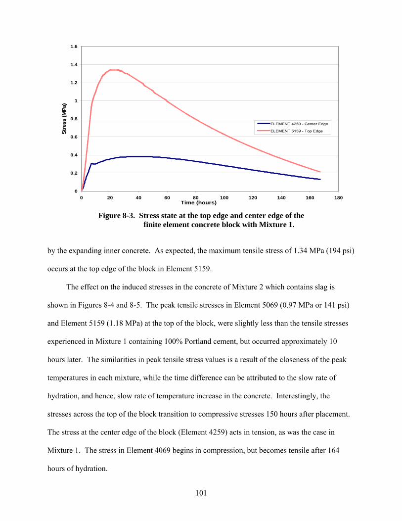
101

0

0.2

0.4

0.6

0.8

1

1.2

1.4

1.6

0 20 40 60 80 100 120 140 160 180Time (hours)

Str

ess

(MP

a)

ELEMENT 4259 - Center Edge

ELEMENT 5159 - Top Edge

Figure 8-3. Stress state at the top edge and center edge of the finite element concrete block with Mixture 1.

by the expanding inner concrete. As expected, the maximum tensile stress of 1.34 MPa (194 psi)

occurs at the top edge of the block in Element 5159.

The effect on the induced stresses in the concrete of Mixture 2 which contains slag is

shown in Figures 8-4 and 8-5. The peak tensile stresses in Element 5069 (0.97 MPa or 141 psi)

and Element 5159 (1.18 MPa) at the top of the block, were slightly less than the tensile stresses

experienced in Mixture 1 containing 100% Portland cement, but occurred approximately 10

hours later. The similarities in peak tensile stress values is a result of the closeness of the peak

temperatures in each mixture, while the time difference can be attributed to the slow rate of

hydration, and hence, slow rate of temperature increase in the concrete. Interestingly, the

stresses across the top of the block transition to compressive stresses 150 hours after placement.

The stress at the center edge of the block (Element 4259) acts in tension, as was the case in

Mixture 1. The stress in Element 4069 begins in compression, but becomes tensile after 164

hours of hydration.

102

-0.6

-0.4

-0.2

0

0.2

0.4

0.6

0.8

1

1.2

0 20 40 60 80 100 120 140 160 180

Time (hours)

Str

ess

(MP

a)



-0.4

-0.2

0

0.2

0.4

0.6

0.8

1

1.2

1.4

0 20 40 60 80 100 120 140 160 180Time (hours)

Str

ess (M

Pa)





103

-0.6

-0.4

-0.2

0

0.2

0.4

0.6

0.8

1

0 20 40 60 80 100 120 140 160 180

Time (hours)

Str

ess

(MP

a)



The stresses produced in Mixture 3 were similar in trend to those obtained in Mixture 1.

This is to be expected given that the rate of temperature rise in Mixture 3 was steep, as was the

case of the temperature rise in Mixture 1. Figure 8-6 shows that the highest tensile stress experi-

enced at the top center of the block (Element 5069) was 0.878 MPa (127 psi) occurring 26 hours

after concrete placement, while the maximum compressive stress of 0.358 MPa (52 psi), at the

center of the block (Element 4069), occurred 40 hours after placement. The maximum tensile

stress value of 1.10 MPa (160 psi) again occurred at the top edge of the block (Element 5159) as

shown in Figure 8-7.

Figure 8-8 shows the stresses calculated in the top center and center of the block contain-

ing Mixture 4, while Figure 8-9 presents the stresses at the edge. The tensile stresses induced in

this block were significantly less than the stresses in Mixture 1and Mixture 3, but slightly larger

than the stresses in Mixture 2. The rate of temperature rise of Mixture 4 like Mixture 2, both of


104

-0.3

-0.2

-0.1

0

0.1

0.2

0.3

0.4

0.5

0 20 40 60 80 100 120 140 160 180

Time (hours)

Str

ess

(MP

a)



0

0.2

0.4

0.6

0.8

1

1.2

0 20 40 60 80 100 120 140 160 180Time (hours)

Str

ess

(MP

a)





105

0

0.1

0.2

0.3

0.4

0.5

0.6

0 20 40 60 80 100 120 140 160 180Time (hours)

Str

ess

(MP

a) ELEMENT 4259 - Center Edge


Figure 8-9. Stress state at the top edge and center edge of the finite element concrete block

with Mixture 4.

which were presented in Chapter 7, was slow. Therefore, this reduction in tensile stresses can

likely be attributed to the presence of the ground granulated blast-furnace slag.

8.2 Cracking Potential

Cracking in concrete will occur when the tensile stresses induced by the temperature

gradients exceed the low tensile strength that exists at early ages. The probability of cracking is

measured by the function presented in Equation 8-1 called the cracking index.

tcr

I

f (t)I (t)

(t)

(8-1)

where Icr = the crack index;

ft = the tensile strength; and

σI = the maximum principal stress.

The crack index (Icr) is given a value of 100 if σI ≤ 0.01ft. If Icr falls below 1.0, this is an

indication that cracking has been initiated.

106

0

10

20

30

40

50

60

70

80

90

100

0 20 40 60 80 100 120 140 160 180

Time (hours)

Cra

ck Index



A plot of the progression of the crack index along the center line of the block in Mixture 1

is presented in Figure 8-10. It shows that almost immediately after the concrete hardens, the

crack index for Element 5069 is less than 1.0, indicating that the tensile stress at the top surface

edge exceeded the tensile strength of the concrete, and hence, cracking has occurred. Element

4069, which is at the center of the block, is always in a compressive state, therefore, has a

constant crack index of 100. Figure 8-11 shows the crack indices for the center edge (Element

4259) and top edge (Element 5159), respectively. Element 4259 remains only just above 1.0,

while Element 5159 shows a high probability that cracking occurs during the first 25 hours. This

was confirmed by a close examination of the experimental block that contained mixture 1, shown

in Figure 8-12, where cracking can be observed at all the top surface edges.

In Mixture 2, cracking occurs at the top center of the block approximately 10 hours after

pouring, as shown in Figure 8-13. The same figure also shows that while the center of block

goes into tension after 80 hours, the concrete is in a mature state and the tensile strength is well

developed. Figure 8-14 shows the crack indices at the edge of the block. As was expected,

Figure 8-10. Crack index for elements along the center line of block with Mixture 1.

107

0

1

2

3

4

5

6

7

8

9

10

11

12

13

14

15

16

17

18

19

20

0 20 40 60 80 100 120 140 160 180

Time (hours)

Cra

ck Index

Element 4259 - Center Edge

Element 5159 - Top Edge

Figure 8-11. Crack index for elements along the edge of block with Mixture 1.

Figure 8-12. Top surface of experimental block containing Mixture 1 showing numerous cracks along the edges.

108

0

10

20

30

40

50

60

70

80

90

100

0 20 40 60 80 100 120 140 160 180

Time (hours)

Cra

ck Index





0

10

20

30

40

50

60

70

80

90

100

0 20 40 60 80 100 120 140 160 180

Time (hours)

Cra

ck Index



109

0

10

20

30

40

50

60

70

80

90

100

0 20 40 60 80 100 120 140 160 180

Time (hours)

Cra

ck Index



cracking occurs at the top edge of the block, however, the center edge of the block just barely

stays above the crack threshold.

Mixtures 3 and 4 act in a similar manner to Mixture 1, where their centers are constantly in

compression, and hence, have negligible risks of cracking. In Mixture 3, the crack indices in

Element 5069 and Element 5159 suggest that cracking will occur, shown in Figures 8-15 and

8-16, respectively, while Figures 8-17 and 8-18 show that, for Mixture 4, the tensile stresses that

develop in these elements will not exceed their tensile strength, and hence, will not crack.

It appears that the ratio of substitution of cementitious materials used in the concrete of

Mixture 4 is effective in mitigating the cracking risk in massive concrete elements.

8.3 Temperature Difference and Cracking

As previously stated, the requirements for the control of heat generation and, in particular

the maximum allowable temperature difference in mass concrete, vary on a state-by-state basis.

Currently, there is no agreement on what the maximum allowable temperature differential should


110

0

10

20

30

40

50

60

70

80

90

100

0 20 40 60 80 100 120 140 160 180

Time (hours)

Cra

ck Index



0

1

2

3

4

5

6

7

8

9

10

11

12

13

14

15

16

17

18

19

20

0 20 40 60 80 100 120 140 160 180

Time (hours)

Cra

ck Index





111

0

2

4

6

8

10

12

14

16

18

20

22

24

26

28

30

0 20 40 60 80 100 120 140 160 180

Time (hours)

Cra

ck Index




be between the center of a mass concrete element and its surface so as to reduce the occurrence

of thermal cracking. The critical temperature differences for the mixtures used in this project are

determined from the results of the finite element analyses on each block.

Figure 8-19 shows the plot of the temperature difference between the center and surface of

the block with Mixture 1. The calculated tensile stresses at the surface exceeded the early age

tensile strength value of 1.25 MPa (181 psi) at a temperature differential of 17.3°C (31.1°F).

Cracking in Mixture 2, which contained ground granulated blast-furnace slag, occurred

when the temperature differential reached about 3.2°C (5.8°F), as shown in Figure 8-20. This is

significantly less than the differential in Mixture 1, which shows that although the addition of

slag to Portland cement slowed the rate of temperature rise, it also caused the concrete to have a

lower early age tensile strength of 0.255 MPa. This was to the detriment of the integrity of the

structure.

112

Figure 8-19. Induced stress with respect to temperature differential for Mixture 1.


113

The temperature differential of 8.4°C (15.1°F) at which cracking initiated in Mixture 3,

shown in Figure 8-21, was larger than the differential in Mixture 2. In this case, although the fly

ash lowered the peak temperature of the concrete, as shown in Figures 7-12 through 7-14, it did

not have any effect on rate of initial temperature rise, and therefore, a low value of the tensile

strength caused the concrete to crack at a lower temperature differential than the block with

Mixture 1.

Figure 8-21. Induced stress with Respect to temperature differential for Mixture 3.

Although the crack index for Mixture 4, presented in Figure 8-17, shows that thermal

cracking does not occur, it was only just avoided. It was, therefore, decided to still investigate

the relationship between the temperature difference and induced stress at the surface of the

block. Figure 8-22 shows the plot of this relationship, and it can be seen that the induced stress

reaches the 24-hour (Day 1) tensile strength of 0.393 MPa, when the temperature differential is

20.6°C (37.1°F), 26 hours after being poured.

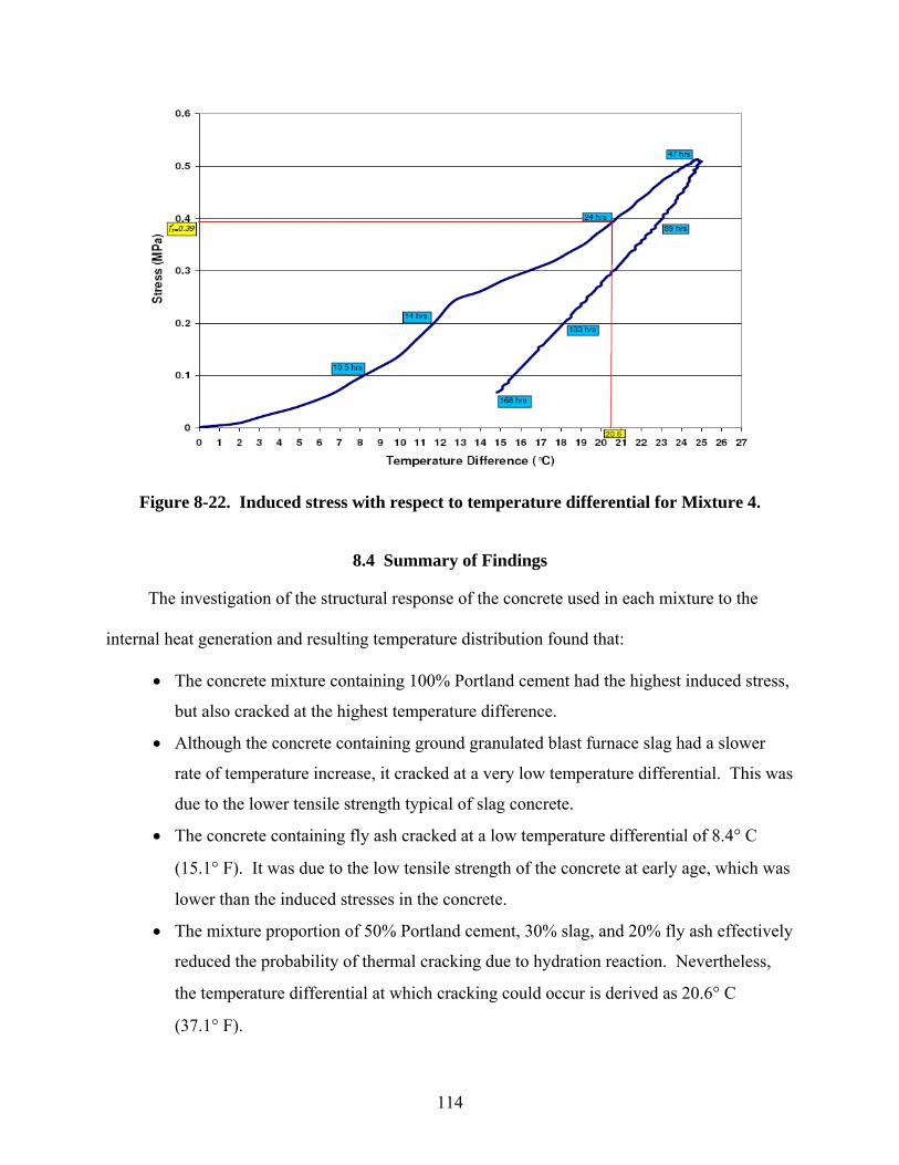
114



The investigation of the structural response of the concrete used in each mixture to the

internal heat generation and resulting temperature distribution found that:

The concrete mixture containing 100% Portland cement had the highest induced stress,

but also cracked at the highest temperature difference.

Although the concrete containing ground granulated blast furnace slag had a slower

rate of temperature increase, it cracked at a very low temperature differential. This was

due to the lower tensile strength typical of slag concrete.

The concrete containing fly ash cracked at a low temperature differential of 8.4°C

(15.1°F). It was due to the low tensile strength of the concrete at early age, which was

lower than the induced stresses in the concrete.

The mixture proportion of 50% Portland cement, 30% slag, and 20% fly ash effectively

reduced the probability of thermal cracking due to hydration reaction. Nevertheless,

the temperature differential at which cracking could occur is derived as 20.6°C

(37.1°F).

115

CHAPTER 9 PARAMETRIC STUDY

9.1 Introduction

This chapter discusses the results of a parametric study conducted with the aid of the

DIANA finite element program. The parameters investigated are effects of the heat generation

rate, size of the structure, and the amount of insulation on the peak temperature, temperature

distribution, and induced stresses in mass concrete structures.

9.2 Effect of Specimen Size

The standard specimen size used in this study was a block size of 1.07 m 1.07 m

1.07m. To study the effect of size on the behavior of concrete, three additional block sizes were

modeled. The sizes chosen were a half-sized block (0.5 m 0.5 m 0.5 m), a block twice the

size (2 m 2 m 2 m), and a block four times the size (4 m 4 m 4 m). A comparison of the

temperature profiles at the center of blocks containing concrete using mix 1 is presented in

Figure 9-1. Figure 9-2 shows the progression of the peak temperatures calculated in the block, as

the size is increased. As expected, the peak temperature increased as the size of the block

increased. A closer analysis of the effect of block size on the maximum temperature difference

is presented in Figure 9-3, where it is shown that the maximum temperature differential between

the center and top surface edge increases from 12.8°C (55.0°F) in the 0.5-m block to 56.5°C

(101.7°F) in the 4-m block. Figures 9-4 and 9-5 are plots of the induced stress at the center of

the top surface and the top surface edge, respectively. In the 1-m 1-m 1-m and the 2-m 2-

m 2-m blocks, the induced stress increases as we move from the center towards the edge of the

blocks. However, in the 4-m 4-m 4-m block, the stresses are the same at the top surface

center and top surface edge suggesting that the stress is constant across the entire surface. The

116

0

10

20

30

40

50

60

70

80

90

100

0 20 40 60 80 100 120 140 160 180

Time (hours)

Tem

per

atu

re (°C

)

0.5m x 0.5m x 0.5m Block1m x 1m x 1m Block2m x 2m x 2m Block4m x 4m x 4m Block

0

10

20

30

40

50

60

70

80

90

100

0.5 1 2 4

Block Size (Length in m)

Peak

tem

per

ature

(°C

)

Figure 9-1. Comparison of temperature profiles calculated at the center of each block.

Figure 9-2. Calculated peak temperature values with respect to block size.

117

0

10

20

30

40

50

60

0.5 1.0 2.0 4.0


Max

imum

Tem

per

taure

Diffe

rence

(°C

)

-0.5

0

0.5

1

1.5

2

2.5

3

3.5

4

0 20 40 60 80 100 120 140 160 180

Time (hours)

Str

ess

(MP

a) 0.5m x 0.5m x 0.5m Block

1m x 1m x 1m Block

2m x 2m x 2m Block

4m x 4m x 4m Block

Figure 9-3. Effect of concrete block size on the maximum internal temperature difference.

Figure 9-4. Comparison of stresses at the center of the top surface of each block.

118

-0.5

0

0.5

1

1.5

2

2.5

3

3.5

4

0 20 40 60 80 100 120 140 160 180

Time (hours)

Str

ess

(MP

a)

0.5m x 0.5m 0.5m Block

1m x 1m x 1m Block

2m x 2m x 2m Block

4m x 4m x 4m Block

Figure 9-5. Comparison of stresses at the top surface edge of each block.

relationship between the maximum induced stress and the increasing maximum temperature

differential caused by increasing block size is presented in Figure 9-6, which shows that for a

given concrete mixture, the maximum induced stress will increase with increasing maximum

temperature differential. Figure 9-7 presents the maximum stress induced in each of the four

types of concrete mixtures that were discussed in the previous chapters with respect to the

maximum temperature difference for each size block. The maximum temperature difference and

resulting stress in concrete elements larger than 1.07 m 1.07 m 1.07 m is highly dependent

on the type of concrete used.

Figure 9-8 shows the maximum induced stress with respect to maximum temperature

gradient in each of the four types of concrete mixtures for each size block. The temperature

gradients in the larger blocks tend to be lower for each type of concrete used in this study. A

comparison of the results presented in Figure 9-7 with those presented in Figure 9-8 show that

119

0

0.5

1

1.5

2

2.5

3

3.5

4

4.5

0 10 20 30 40 50 60 70 80

Maximum Temperature Difference (°C)

Max

imum

Str

ess

(MP

a)

0.5m x 0.5m x 0.5m

1m x 1m x1m

2m x 2m x 2m

4m x 4m x 4m

Linear (0.5m x 0.5m x 0.5m)

Linear (1m x 1m x1m)

Linear (4m x 4m x 4m)

Linear (2m x 2m x 2m)

Figure 9-6. Maximum induced stress with respect to maximum temperature differential as a result of increasing block size.

Figure 9-7. Plot of maximum stress versus maximum temperature difference with respect to block size and type of concrete used.

120

0

0.5

1

1.5

2

2.5

3

3.5

4

4.5

0 10 20 30 40 50 60 70

Maximum Temperature Gradient (°C/m)

Max

imum

Str

ess

(MP

a)0.5m x 0.5m x 0.5m

1.0m x 1.0m x 1.0m

2.0m x 2.0m x 2.0m

4.0m x 4.0m x 4.0m





Figure 9-8. Plot of maximum stress versus maximum temperature gradient with respect to block size and type of concrete used.

while maximum stress appears to be a function of temperature difference regardless of block

size, it is not a function of temperature gradient alone. It appears that temperature difference,

rather than temperature gradient, is a better indicator of maximum stress in mass concrete.

9.3 Effect of Insulation Thickness

Two model blocks, one insulated 1.5-in. thick layer of polystyrene foam, and the other

with a 6-in. thick layer polystyrene foam, were created, analyzed, and their results compared

with the model analyzed in the previous chapters, to quantify the effect that the amount of

insulation would have on the temperature distribution in a hydrating concrete element containing

100% Portland cement. Figures 9-9 and 9-10 present the temperature profiles with respect to

time of the concrete block insulated with 1.5-in. thick and 6-in. thick layers of polystyrene foam,

respectively. The block with the 1.5-in. thick layer of insulation had a maximum temperature

121

0

10

20

30

40

50

60

70

80

0 20 40 60 80 100 120 140 160 180

Time (hours)

Tem

per

ature

(°C

)

2" Below Top Surface



0

10

20

30

40

50

60

70

80

0 20 40 60 80 100 120 140 160 180

Time (hours)

Tem

per

ature

(°C

)




Figure 9-9. Temperature profiles with respect to time 2 in., 4 in., and 21 in. below the top

surface of the block insulated with a 1.5-in. thick layer of polystyrene foam.

Figure 9-10. Temperature profiles with respect to time 2 in., 4 in., and 21 in. below the top

surface of the block insulated with a 6.0-in. thick layer of polystyrene foam.

122

difference between the center of the block and a point 2 in. below the exposed top surface of

14.9°C (26.8°F), occurring 32 hours after casting and was maintained for 7 hours before

steadily decreasing to 3.6 °C (6.5°F). The maximum temperature difference between the center

and a point 2 in. below the exposed top surface calculated in the block with the 6-in. layer of

insulation was 20°C (36°F). This maximum difference was attained after 70 hours of

hydration, slowly decreasing to 15.8°C (28.4°F) at the end of the analysis at 167 hours.

Figure 9-11 shows the comparison of the temperatures with respect to time 2 in. below

the exposed top surface of the concrete blocks with varying insulation thickness. The peak

temperature at this location was found to be the same and occurred at the same time in all three

blocks. However, the rate of temperature decrease was slowest in the model with the 6-in.

insulation, and fastest in the model with the 1.5-in. insulation. The temperatures 4 in. below the

top surface presented in Figure 9-12 were similar to those observed at 2 in. in terms of the three

blocks attaining the same peak temperature at approximately the same time but having different

rates of decline.

The comparison of the temperatures 21 in. below the top surface are shown in Figure 9-13.

At this depth, the peak temperature and the time it is attained increase in accordance with the

thickness of the polystyrene foam.

Although the top surface of the blocks modeled in this project were exposed to ambient

conditions, the effectiveness of the insulation in reducing temperature differences within the

concrete varied with respect to its thickness. This was determined by evaluating the temperature

difference between the center of the block and a point at the same depth, but on the side of the

block. Figure 9-14 shows the temperature in the concrete block modeled with the 1.5-in. thick

polystyrene insulation, where a maximum temperature difference of 8.3°C (14.9°F) between the

123

0

10

20

30

40

50

60

0 20 40 60 80 100 120 140 160 180

Time (hours)

Tem

per

atu

re (°C

)

1.5 Inch Thick Insulation



0

10

20

30

40

50

60

70

0 20 40 60 80 100 120 140 160 180

Time (hours)

Tem

per

ature

(°C

)




Figure 9-11. Comparison of temperature profiles with respect to time 2 in. below the top surface of the blocks with varying thicknesses of polystyrene foam insulation.

Figure 9-12. Comparison of temperature profiles with respect to time 4 in. below the top surface of the blocks with varying thicknesses of polystyrene foam insulation.

124

0

10

20

30

40

50

60

70

80

0 20 40 60 80 100 120 140 160 180

Time (hours)

Tem

per

atu

re (°C

)




0

10

20

30

40

50

60

70

80

0 20 40 60 80 100 120 140 160 180

Time (hours)

Tem

per

ature

(C

)

Side

Center

Figure 9-13. Comparison of temperature profiles with respect to time 21 in. below the top

surface of the blocks with varying thicknesses of polystyrene foam insulation.

Figure 9-14. Temperatures calculated at the side and center of a concrete block with 1.5-in.

thick insulation.

125

center and the side is observed. The temperatures in the block with the 3-in. thick polystyrene

insulation are presented in Figure 9-15. Here, the maximum temperature difference between the

two points decreases to 3.4°C (6.1°F). Figure 9-16, shows that for the block insulated with a

6-in. thick layer of polystyrene, the temperature difference was only 1.9°C (3.4°F).

Having assessed the effects of the insulation thickness on the temperature distribution in

the uncovered block, an investigation on the effect of the insulation thickness on the maximum

temperature differential and maximum induced stress in a concrete block insulated on all faces

was conducted. Figures 9-17 and 9-18 show comparisons of the experimentally measured and

numerically calculated temperature profiles at 2 in. and 4 in. below the top surface of the fully

insulated concrete block with Mixture 1 for validation purposes.

Figure 9-18 presents the variation in maximum temperature differential within the concrete

with respect to insulation thickness. Figure 9-19 also shows how the block size determines the

effect increasing the insulation thickness will have on the maximum temperature differential

within the concrete. As shown in Figure 9-19, increasing the insulation thickness from 1.5 in. up

to 9 in. will reduce the temperature difference between the center and top surface of the block.

In the 0.5-m block, the maximum temperature difference moved from 5.6°C (10.1°F) with 1.5

in. of insulation, to 4.2°C (7.6°F) with 3 in. of insulation, to 3.2°C (5.8°F) with 6 in. of

insulation, to 2.8°C (5.0°F) with 9 in. of insulation. The 1.07-m block had values of 12.4°C,

8.9°C, 6.5°C, and 5.4°C (22.3°F, 16.0°F, 11.7°F, and 9.7°F) with insulation thicknesses of

1.5 in., 3 in., 6 in., and 9 in., respectively. The 2-m block had a temperature difference of

22.8°C (41.0°F) at 1.5 in., 16.7°C (30.1°F) at 3 in., 11.6°C (20.9°F) at 6 in., and 9.3°C

(16.7°F) at 9 in. Finally, the 4-m block saw the largest reduction in the magnitude of the

maximum temperature difference with increasing insulation thickness. The maximum

126

0

10

20

30

40

50

60

70

80

0 20 40 60 80 100 120 140 160 180

Time (hours)

Tem

per

ature

(C

)

Side

Center

0

10

20

30

40

50

60

70

80

0 20 40 60 80 100 120 140 160 180

Time (hours)

Tem

per

ature

(C

)

Side

Center


thick insulation.


thick insulation.

127

0

10

20

30

40

50

60

70

80

0 20 40 60 80 100 120 140 160 180

Time (hours)

Tem

per

atu

re (°C

)


Experimental

0

10

20

30

40

50

60

70

80

0 20 40 60 80 100 120 140 160 180

Time (hours)

Tem

per

atu

re (°C

)


Experimental

Figure 9-17. Comparison of experimentally measured and calculated temperature profiles

2 in. below the top surface at the centerline of concrete block with 3.0-in. thick insulation.

Figure 9-18. Comparison of experimentally measured and calculated temperature profiles

4 in. below the top surface at the centerline of concrete block with 3.0-in. thick insulation.

128

0

5

10

15

20

25

30

35

40

0 1 2 3 4 5 6 7 8 9 10

Insulation Thickness (inch)

Max

imum

Tem

per

ature

Diffe

rence

(°C

)0.5m x 0.5m x 0.5m Block

1m x 1m x 1m Block

2m x 2m x 2m Block

4m x 4m x 4m Block

Figure 9-19. Variation in maximum temperature differential within the concrete with respect to insulation thickness for each block size.

temperature difference in the block with 1.5 in. of insulation was calculated at 37.7°C (67.9°F),

with 3 in. of insulation, 27.2°C (49.0°F), 6 in. of insulation, 18.1°C (32.6°F), and finally, with

9 in. of insulation, 14°C (25.2°F).

Figures 9-20 and 9-21 show the effect of increasing the insulation thickness had the

maximum induced stress in the concrete with respect to temperature difference. Figure 9-20

shows that the reduced magnitude of temperature difference caused by an increase in insulation

thickness will result in lower induced stress within the concrete block. Figure 9-21 shows that

by increasing the insulation thickness, significant reductions in stresses can be achieved in large

concrete elements.

9.4 Time of Formwork Removal Effect

The effect model was modified so that the effect that the time of removal of the formwork

had on the induced concrete stresses could be assessed. Knowledge of the optimal time to

129

0.0

0.5

1.0

1.5

2.0

2.5

3.0

3.5

4.0

4.5

0 5 10 15 20 25 30 35 40

Maximum Temperature Difference (°C)

Max

imum

Str

ess

(MP

a)


3 Inch Thick Insulation



0

0.5

1

1.5

2

2.5

3

3.5

4

4.5

0 0.5 1 1.5 2 2.5 3 3.5 4 4.5


Maxi

mum

Str

ess (M

Pa)

1.5 Inch Insulation

3.0 Inch Insulation

6.0 Inch Insulation

9.0 Inch Insulation

Figure 9-20. Effect of reduction of temperature differential caused by increasing insulation thickness on the maximum induced stress.

Figure 9-21. Effect of insulation thickness on the maximum induced stress in each block size.

130

remove the formwork and insulation around mass concrete is important in that the scheduling of

the construction time sequence is an essential aspect of project management. The times chosen

for analysis were 12 hours, 1 day, 2 days, 3 days, 4 days and 6 days after pouring of the concrete.

Figures 9-22 through 9-27 show the induced stress with respect to time in a 1.07-m

1.07-m 1.07-m concrete block concrete when the formwork and insulation is removed at times

of 12 hours, 1 day, 2 days, 3 days, 4 days and 6 days.

A sharp sudden increase in tensile stress occurred along the surface immediately after

formwork removal. The peak stress calculated for the removal times at 12 hours, 1 day, 2 days,

and 3 days, were 0.964 MPa, 1.08 MPa, 1.31 MPa, 1.30 MPa, respectively. These were 77%

86.4%, 79%, and 67.4% of the attained concrete tensile strength, respectively. While not

exceeding the tensile strength of the concrete, these stress levels are high enough to cause micro-

cracking. These micro-cracks do not pose an immediate threat to the structural integrity of the

concrete, however, they will provide an entry point for invasive deleterious substances that can

compromise the long-term durability of the concrete. Figure 9-26 shows the state of stress in

concrete when the formwork is removed after 4 days of hydration. The stress also undergoes a

sharp increase in magnitude the instant the formwork is removed, but is only slightly above 50%

of the tensile strength at 4 days, therefore the risk of micro-cracking is small. Figure 9-27 shows

the stresses for the concrete that had the formwork and insulation removed after 6 days of

hydration. Here, the peak stress of 1.08 MPa is 49% of the tensile strength of the concrete.

The results of the parametric study on the effect time of formwork and insulation removal

suggests that the risk of micro-cracking is substantially reduced if the removal is done a mini-

mum of 4 days after the concrete is poured.

131

-0.2

0

0.2

0.4

0.6

0.8

1

1.2

0 20 40 60 80 100 120 140 160 180Time (hours)

Str

ess

(M

Pa)

ELEMENT 5213 Removed 12 hours

ELEMENT 5213 No Removal

-0.4

-0.2

0

0.2

0.4

0.6

0.8

1

1.2

0 20 40 60 80 100 120 140 160 180

Time (hours)

Str

ess

(MP

a) ELEMENT 5213 Removed 24 hours


Figure 9-22. Plot of stress versus time at a point on the center of the surface of the concrete

block when formwork is removed 12 hours after casting.


block when formwork is removed 1 day after casting.

132

-0.2

0

0.2

0.4

0.6

0.8

1

1.2

1.4

0 20 40 60 80 100 120 140 160 180

Time (hours)

Str

ess

(MP



-0.2

0

0.2

0.4

0.6

0.8

1

1.2

1.4

0 20 40 60 80 100 120 140 160 180

Time (hours)

Str

ess

(MP




block when formwork is removed 2 days after casting.



133

-0.2

0

0.2

0.4

0.6

0.8

1

1.2

1.4

0 20 40 60 80 100 120 140 160 180

Time (hours)

Str

ess

(MP

a)



0

0.2

0.4

0.6

0.8

1

1.2

0 20 40 60 80 100 120 140 160 180

Time (hours)

Str

ess

(MP

a)







134

0

10

20

30

40

50

60

70

80

0 20 40 60 80 100 120 140 160 180

Time (hours)

Tem

per

atu

re (°C

)

100% Portland Cement

50% Portlan Cement 50% Slag

65% Portland Cement 35% Fly Ash

50% Portland 30% Slag 20% Fly ash

9.5 Heat Generation Rate Effect

The effect the rate of internal heat generation has on the distribution of temperatures in a

concrete element can be seen from the analysis of the block model with varying mixture designs

described in Chapter 7. It was observed that concrete with 100% Portland cement generated heat

at the fastest rate, followed by the concrete with 35% replacement of fly ash, then by the substi-

tution of 50% ground granulated blast-furnace slag, and the slowest rate of heat generation

occurred in the mixture with 50% Portland cement, 30% slag, and 20% fly ash (ternary blend).

Figure 9-28 shows the temperature profile with respect to time at the center of the concrete

blocks containing each mix. It is seen that the concrete containing the highest rate of heat

generation (100% Portland cement) had the sharpest rise in temperature and the highest peak

temperature. The ternary blend concrete with the slowest rate of heat generation had the lowest

temperature rise slope and also the lowest peak temperature.

Figure 9-28. Temperature profiles with respect to time at the center of a concrete block with varying heat generation rates.

135


The parametric study of the factors affecting the behavior of concrete resulted in the

following:

The peak temperature, internal temperature gradients, and induced thermal stresses

increase as the amount of concrete used in any one pour is increased.

The thickness of the insulating layer around the block formwork has an indirect effect

on the magnitude of the maximum temperature difference in the hydrating concrete.

For a given resistance value (R-Value) of an insulating material, the temperature

difference in concrete will decrease with increasing insulation thickness.

Concrete with a fast rate of heat generation will have higher peak temperatures

increasing the likelihood that thermal cracking will occur.

The effectiveness of insulation thickness in the reduction of the maximum temperature

differential in concrete is dependent on the size of the concrete block. An increase in

insulation thickness from 1.5 in. to 9 in. reduced the maximum temperature differential

by 50% in a 0.5-m 0.5-m 0.5-m block while the reduction in a 4-m 4-m 4-m

block was 62.9%.

Increasing the insulation thickness can achieve significant reductions in thermal

stresses in large concrete elements.


at 12 hours, 1 day, 2 days, and 3 days after pouring of the concrete were less than the

tensile strength of the concrete as measured in the laboratory, the stresses were large

enough to initiate micro-cracking. These micro-cracks can serve as an entry point for

deleterious materials that can undermine the durability of the concrete.

136

CHAPTER 10 RECOMMENDED TESTING REGIMEN

FOR MASS CONCRETE

10.1 Recommended Testing Method for Measurement

of Heat Generation

Three calorimetry methods were investigated for the measurement of heat generation in

concrete materials: isothermal conduction calorimetry, semi-adiabatic calorimetry, and Sure-

Cure/adiabatic calorimetry. Of the three methods investigated, the isothermal calorimetry

method was determined to be the most appropriate method for the quantification of heat

generation of cementitious materials at early ages. There are several reasons as to why the

isothermal calorimetry method was favored over the other calorimetry techniques. Firstly, the

isothermal calorimetry method provided the most accurate and repeatable results for the

measurement of the heat generation of cementitious materials. Secondly, the results provided by

the isothermal calorimetry are in units of power (mW/g) and energy (J/g). Although this

research established some baseline values for the specific heat capacity of the ingredients used to

make concrete, there are potential errors in those values which could provide erroneous results in

the conversion from temperature rise as measured by semi-adiabatic and adiabatic calorimetry.

Thirdly, the isothermal conduction calorimeter is commercially available and standardization of

the test method for the determination of energy rise of cementitious materials is imminent.

Finally, there have been some recent developments in modeling/prediction software programs

which utilize the energy rise data for cementitious materials for input parameters. Therefore, the

use of the isothermal conduction calorimeter is recommended for the measurement of

heat/energy rise of concrete for the purposes of prediction of the behavior of mass concrete.

137

10.2 Recommended Testing Method for Measuring Maturity/Equivalent Age

The laboratory testing method for the establishment of maturity and equivalent age

relationships based on the time-temperature history falls under ASTM 1074. The relative

strength relationships developed by the maturity method (ASTM 1074-6.2) also known as the

Nurse-Saul maturity method, did not yield accurate results. Therefore, it is recommended not to

use the Nurse-Saul method for the prediction of strength properties of mass concrete.

The standardized equivalent age method developed relative strength relationships per

ASTM 1074-6.3 (also known as the Arrhenius equation), which utilized a hyperbolic mathe-

matical model for the evolution of compressive strength of mortar cubes. This research

investigated a second equivalent age method (Schindler 2002) which utilized the compressive

strength of mortar cubes as well, but used an exponential mathematical model rather than the

model prescribed in ASTM 1074.6.3 (hyperbolic method) for the establishment of activation

energy (Ea). A third method for the establishment of equivalent age and Ea was investigated

utilizing isothermal calorimetry of cementitious material in lieu of compressive strength testing

of mortar cubes. As previously stated, the isothermal calorimetry test is required for the

determination of the measurement of heat generation characteristics of the cementitious

materials. Accordingly, it is possible to use the data obtained from isothermal calorimetry

testing (for heat generation) to determine the Ea of the cementitious material. Therefore, the

compressive strength testing per ASTM 1074 would not be needed for the determination of Ea, if

the isothermal calorimetry testing was used in its place.

Each of the three equivalent age techniques produced accurate results for the prediction of

the relative strength of concrete which utilized Portland cement as the only cementitious

material. However, initial testing indicated that the Ea results obtained by the isothermal testing

138

method were the most accurate for cementitious materials in which Portland cement was

replaced with a large percentage of supplementary cementitious material (35-50%). However,

the current models established for equivalent age relationships for concrete with large amounts

of supplementary cementitious materials do not adequately predict the behavior of relative

strength of concrete.

Therefore, the equivalent age relationships should be used to predict the strength behavior

of concrete. Following the results obtained in this research, the Ea, as calculated via isothermal

calorimetry testing and the standardized test method, may be used for the prediction of concrete

with large replacement of SCM. However, the models do not adequately predict the behavior of

relative strength of concrete with large replacements of SCM.

10.3 Recommended Testing Methods for Strength

and Modulus of Elasticity

10.3.1 Compressive Strength

The most commonly measured property of hardened concrete is compressive strength. The

FDOT specification requires a standardized minimum compressive strength, at an age of 28 days

of all structural concrete used in the State of Florida. Thus, the compressive strength has become

the fundamental strength test for concrete. Despite the fact that mass concrete will rarely

experience failure in a compressive manner, it is recommended to perform compressive strength

testing of concrete for acceptance and comparative purposes.

10.3.2 Compressive Modulus of Elasticity

The modulus of elasticity is the most important strength parameter for the prediction of the

behavior of mass concrete. Near surface tensile strains (as predicted by CTE measurements),

due to the expansion of the hotter inner core of mass concrete, can be used to calculate tensile

139

stress, if the modulus of elasticity is known. Therefore, the modulus of elasticity is an important

parameter for the prediction of potential thermal/tensile cracking of mass concrete.

The compressive modulus of elasticity test is the only standardized test for measurement of

the modulus of elasticity for concrete. The findings of this research indicate that the compressive

modulus of elasticity is approximately the same as the tensile (flexural) modulus of elasticity

when tested at loads of 33% of ultimate. Therefore, the modulus of elasticity measured

compressively can be considered the same value for the tensile modulus of elasticity for

prediction and modeling purposes of mass concrete. Therefore, it is not necessary to determine

tensile/flexural modulus of elasticity via laboratory testing.

10.3.3 Tensile Strength

Tensile strength is particularly important for the prediction of mass concrete since the

failure of mass concrete at early ages is typically tensile in nature. Near surface tensile stresses

(as predicted by CTE) and modulus of elasticity measurements of mass concrete (as predicted by

modeling software) can be compared with tensile strength obtained via laboratory testing.

Accordingly, the prediction of cracking can be established with respect to the expansive nature

(due to temperature rise or temperature differentials) within the mass concrete. When the

predicted tensile stress exceeds the ultimate tensile stress of the concrete obtained by laboratory

testing, cracking will occur.

10.4 Recommended Testing Method for Measurement

of Coefficient of Thermal Expansion

The coefficient of thermal expansion of concrete is perhaps the most important parameter

to accurately quantify with respect to mass concrete. Currently, the standardized method for the

measurement of CTE (AASHTO TP-60-2007) has been withdrawn due to the potential concerns

with the calibration factor (of stainless steel) used to calibrate the test (Crawford 2009).

140

Therefore, the results obtained under this research were calculated per the calibration testing

performed at the FDOT SMO. Considering the recent developments and potential problems

regarding the CTE test method, it is recommended to perform CTE testing in the laboratory for

the prediction of mass concrete. Furthermore, it should be noted that early-age CTE is a

necessary parameter to properly establish and consider its variability in the prediction of the

behavior of mass concrete.

10.5 Recommended Physical Parameter

for the Concrete Diffusivity

The thermal diffusivity testing reported in this research indicates that the thermal

diffusivity values for concrete at early ages range from 0.513 ft2/day to 0.748 ft2/day, whereas

the thermal diffusivity of concrete made with limestone aggregate as reported by ACI 207.2 is

1.22ft2/day. The reason for the difference in the diffusivity values obtained in this research, and

those obtained by ACI 207.2, is due to the coarse aggregate within the concrete. Therefore, the

values for thermal diffusivity reported in this research should be used for the prediction of mass

concrete which incorporate coarse aggregate from Florida. However, for concrete created with

coarse aggregate from elsewhere, the values per ACI 207.2 should be considered for the predic-

tion of the behavior of mass concrete.

10.6 Recommended Physical Parameter for

the Specific Heat Capacity

The specific heat capacity testing reported in this research indicates that the specific heat

capacity values for concrete at early ages range from 1.1 to 1.2 J/(g-°C), whereas the specific

heat capacity of concrete made with limestone aggregate as reported by ACI 207.2 is 0.91 to

1.05 J/(g-°C). The reason for the difference in the diffusivity values obtained in this research,

and those obtained by ACI 207.2, is due to the coarse aggregate within the concrete. Similar to

141

the results obtained for thermal diffusivity, the specific heat capacity values reported in this

research should be used for the prediction of behavior of mass concrete which incorporates

coarse aggregate from Florida. However, for concrete created with coarse aggregate from

elsewhere, the values per ACI 207.2 should be considered for the prediction of the behavior of

mass concrete.

10.7 Summary of Testing Program

The laboratory testing program for the prediction of the behavior of mass concrete should

include the following tests:

1) Isothermal calorimetry for the measurement of heat generation rate;

2) Compressive strength per ASTM 1074 or isothermal calorimetry testing for the

determination of activation energy;

3) Compressive strength of concrete cylinders;

4) Splitting tensile strength of concrete cylinders;

5) Compressive modulus of elasticity at 30% of ultimate strength (for the determination

of tensile modulus of elasticity);

6) Coefficient of thermal expansion; and

7) Thermal diffusivity and specific heat capacity.

142

CHAPTER 11 CONCLUSIONS AND RECOMMENDATIONS

11.1 Findings

A finite element model was built to predict the early age behavior of hydrating concrete

element. To validate the accuracy of the model and hence verify the results obtained from the

model, four different concrete mixtures were used in experimental blocks with dimensions 3.5 ft.

3.5 ft. 3.5 ft. (1.07 m 1.07 m 1.07 m) and monitored for temperature distributions. The

material and physical properties of the concretes used were obtained from laboratory testing and

used in the finite element model. The two types of tests done on the concrete mixtures to deter-

mine the energy released during hydration were semi-adiabatic calorimetry and isothermal

calorimetry. The calculated adiabatic energy rise obtained from each test was used in the model

to determine which procedure would give the best results when compared with the temperatures

measured in the experimental block.

Based on the results of the thermal analysis of the concrete block model, the following

findings were made:

The semi-adiabatic calorimetry test consistently gave lower heat of hydration and

lower predicted temperature of concrete as compared with the isothermal calorimetry

test.

The input of adiabatic energy captured in the isothermal calorimetry test provided

temperature distributions that were very similar to those measured in the experimental

blocks. At some locations, the predicted temperatures were higher than the measured

temperatures, and so the isothermal test can be said to provide conservative predictions

of the temperature distribution.

The induced stresses caused by the varying temperatures within the concrete element of

each mixture were analyzed using the results from the model that utilized the energy from

143

isothermal calorimetry test. The magnitude and type of stresses were of particular interest in

determining the likelihood of thermal cracking. The results of this structural analysis for the

concrete block study led to the following observations:

The highest tensile stresses were located at the top edge of the surface exposed to

ambient conditions.

Concrete containing 100% Portland cement experienced tensile stresses high enough to

cause cracking on all surfaces, even those insulated, when the temperature difference

was 17.3°C (31.1°F).

In the case where 50% of the Portland cement was replaced with ground granulated

blast-furnace slag, the rate of hydration reaction and, hence rate of temperature

increase, was significantly slower. The associated reduction in early age tensile

strength resulted in the cracking risk not being reduced.

In the case where 35% of the Portland cement was substituted with fly ash, there was

little effect on the early age rate of hydration, and thus, the time in which the maximum

temperature was achieved was not affected significantly. However, the maximum

temperature achieved was itself significantly less. Again, the early age tensile strength

was less than the 100% Portland cement case, resulting in similar cracking on all

surfaces as before, even though the tensile stresses experienced were less.

Concrete that had a blend of 50% Portland cement, 30% slag, and 20% fly ash

performed the best in terms of reducing the induced thermal stresses relative to the

tensile strength, and hence, the cracking potential.

The temperature differential that induced cracking in the concretes used in this project

varied from mixture to mixture. This was due to the corresponding changes in the

tensile strength.

The parametric study on factors affecting the temperature distribution in concrete produced

very interesting results as follows:

The thermal stresses in large mass concrete elements were effectively reduced with the

use of thick layers of insulating polystyrene foam. This method is advantageous

144

because the polystyrene foam, if removed carefully, can be reused often making it

relatively inexpensive when compared to other single use methods such as cooling

pipes and liquid nitrogen.


12 hours, 1 day, 2 days, and 3 days after the pouring of the concrete were less than the

tensile strength of the concrete as measured in the laboratory, the stresses could be

large enough to initiate micro-cracking. These micro-cracks can serve as an entry point

for deleterious materials that can undermine the durability of the concrete. For

insulation removed after 4 days, the tensile stresses were significantly less than the

tensile strength, reducing the risk of micro-cracking.

11.2 Conclusions

Based on the results obtained in this study, the following conclusions are made:

The heat of hydration energy data obtained from the isothermal calorimetry test should

be used for the input for the heat generation function in the finite element modeling of

concrete hydration.

Reliance on a limiting maximum temperature differential to control cracking in

massive concrete applications should be supplemented with a requirement for the

presentation of a finite element analysis showing the calculated stress response to the

predicted temperature distribution within the concrete, to ensure that the induced

tensile stresses will not exceed the tensile strength of the concrete.

Adequate insulation should be used in conjunction with the usual formwork material to

reduce the temperature differentials during the early age hydration of massive concrete.

However, caution should be taken, as the occurrence of delayed ettringite formation

(DEF) and drying shrinkage due to high concrete temperatures was not studied.

A safety factor should be applied to the tensile strength values for concrete obtained

from the splitting tension and third-point flexural strength tests to guard against the

initiation of micro-cracks which, although by themselves will not cause structural

failure, can act as an entry point for deleterious materials which can undermine the

durability of the concrete.

145

The current restrictions on maximum temperature imposed by state regulating bodies

should take into consideration the type of cementitious materials that will be used in

the concrete mix.

11.3 Recommendations for Future Research

It is recommended that additional blends of cementitious materials and additional larger

blocks of mass concrete be tested in order to assess the universal applicability of the hypotheses

deduced and concluded from this study.

146

LIST OF REFERENCES ACI Committee 207. (2005). 207.1R-05: Guide to Mass Concrete, Farmington Hill, MI.

ACI Committee 207. (2005). 207.2R-07: Report on Thermal and Volume Change Effects on Cracking of Mass Concrete, Farmington Hills, MI.

Ayotte, E., Massicotte, B., Houde, J., and Gocevski, V. (1997). “Modeling of Thermal Stresses at Early Ages in a Concrete Monolith.” ACI Materials Journal, Vol. 94, No. 6, p. 577-587.

Bamforth, P.B. (1984). “Mass Concrete.” Concrete Society Digest. Concrete and Cement Association.

Bhatty, J.I., and Taylor, P.T. (2006). Sulfate Resistance of Concrete Using Blended Cements or Supplementary Cementitious Materials. Portland Cement Association, Skokie, IL.

Boyd, A.J., and Mindess, S. (2002). An Indirect Tension Test for Concrete, Fifth International Symposium on Cement & Concrete. Tongji University Press, Shanghai, China, Vol. I, pp. 590-594.

Boyd, A.J., and Mindess, S. (2004). “The Use of Tension Testing to Investigate the Effect of W/C Ratio and Cement Type on the Resistance of Concrete to Sulfate Attack.” Cement and Concrete Research. Elsevier, Vol. 34, No. 3, pp. 373-377.

Bremner, T.W., Boyd, A.J., Holm, T.A., and Boyd, S.R. (1998). “Indirect Tensile Testing to Evaluate the Effect of Alkali-Aggregate Reaction in Concrete.” Proceedings, Structural Engineering World Wide. ASCE, San Francisco, CA, CD-ROM Paper T192-2, 12 pp.

Chini , A.R., Muszynski, L.C., Acquaye, L., and Tarkhan, S. (2003). Determination of the Maximum Placement and Curing Temperatures in Mass Concrete to Avoid Durability Problems and DEF. FDOT Contract BC-354-29. Florida Department of Transportation, Tallahassee, February.

Crawford, G. (2009). “Concrete Coefficient of Thermal Expansion.” Presentation to AASHTO Joint Technical Committee on Pavements. Jackson Hole, WY, May 27-28.

De Schutter, G., and Taerwe, L. (1995). “General Hydration Model for Portland Cement and Blast Furnace Slag Cement.” Cement and Concrete Research, Vol. 25, No. 3, pp. 593-604.

De Schutter, G., and Taerwe, L. (1995). “Specific Heat and Thermal Diffusivity of Hardening Concrete.” Mag. Concr. Res., Vol. 47, No. 172, pp. 203-208.

Divet, L., and Pavione, A. (2002). “Delayed Ettringite Formation in Massive Concrete Structure:, an Account of Some Studies of Degraded Bridges.” Proceedings, International RILEM TC 186-ISA Workshop, RILEM. Villars, Switzerland, pp. 98-126.

147

Drimalas T. (2004). “Laboratory Testing and Investigations of Delayed Ettringite Formation.” Masters Thesis. University of Texas, Austin, TX.

Florida Department of Transportation. (2007). Standard Specifications for Road and Bridge Construction. Florida Department of Transportation (FDOT), Tallahassee.

Florida Department of Transportation. (2009). FDOT Structures Manual. Florida Department of Transportation (FDOT), Tallahassee.

Gajda, J. (2007). Mass Concrete for Buildings and Bridges. Portland Cement Association, Skokie, IL.

Ghorab, H.Y. (2002). “On the Chemistry of Delayed Ettringite Formation.” Proceedings, International RILEM TC 186-ISA Workshop, RILEM. Villars, Switzerland, pp. 65-81.

Higginson, E.C. (1970). “The Effect of Cement Fineness on Concrete. Fineness of Cement. STP 473. American Society for Testing and Materials (ASTM), Philadelphia, PA, pp. 71-81.

Kelham, S. (2002). “Effects of Cement Parameters on Expansion Associates with DEF.” Proceedings, International RILEM TC 186-ISA Workshop, RILEM. Villars, Switzerland, pp. 98-126.

Lane, D.S., and Ozyildrirm, H.C. (1999). “Evaluation of the Potential for Internal Sulfate Attack Through Adaptation of ASTM C 342 and the Duggan Test Cement.” Concrete & Aggregates, ASTM, Vol. 21, No. 1, pp. 43-58.

Larsen, T.J. (1991). The Effects of Variation in Tricalcium silicate of Portland Cement on Concrete Properties. August 1989, Revised Feb 1991, Florida Department of Transportation, Tallahassee.

Lawrence, C.D. (1998). Physiochemical and Mechanical Properties of Portland Cements, Lea’s Chemistry of Portland Cement. 4th Edition. Arnold Publisher, Edited by P.C. Hewlett, pp. 343-349.

Lindstrom, L., and Westerberg, B. (2003). “Fine Ground Cement in Concrete - Properties and Prospects.” ACI Materials Journal, Vol. 100, No. 5, pp. 398-406.

Machida, N., and Uehara, K. (1987). “Nonlinear Thermal Stress Analysis of a Massive Concrete Structure.” Comput. Struct., Vol. 26, pp. 287-296.

Malhotra, V.M., and Mehta, P.K. (1996). Pozzolanic and Cementitious Materials. Gordon and Breach Publishers, Canada.

Mehta, P.K., and Monteiro, P. J. M. (2006). Concrete – Microstructure, Properties and Materials. 3rd Edition. McGraw-Hill.

148

Miller, F. M., and Conway, T. (2003). “Use of Ground Blast Furnace Slag for the Reduction of Expansion Due to Delayed Ettringite Formation.” Cement, Concrete & Aggregates, ASTM, Vol. 25, No. 1, pp. 43-58.

Neville, A. (1995). Properties of Concrete. 4th Edition. Essex, England Pearson Education Limited.

Poole, T. (2004). Predicting Heat of Hydration in Hydraulic Cement. U.S. Army Research and Development Center, Vicksburg, MS, April.

Price, W.H. (1974). “Practical Qualities of Cement.” Journal of the American Concrete Institute, Vol. 71, No. 9, September, pp. 436-444.

Radovanic, S. (1998). Thermal and Structural Finite Element Analysis of Early Age Mass Concrete Structures. University of Manitoba, Winnipeg, Manitoba, Canada.

Ramlochan, T., Zacarias, P., Thomas, M..D.A., and Hooton, R.D. (2003). “The Effect of Pozzolans and Slag on the Expansion of Mortars Cured at Elevated Temperature, Part I: Expansive Behaviour.” Cement and Concrete Research, Elsevier, Vol. 33, pp. 807-814.

RILEM 119-TCE 1. (1997). “Adiabatic and Semi-Adiabatic Calorimetry to Determine the Temperature Increase in Concrete Due to Hydration Heat of Cement.” Materials and Structures, Vol. 30, pp. 451-457.

Schindler, A.K. (2002). “Concrete Hydration, Temperature Development, and Setting at Early Ages.” Ph.D. Dissertation. University of Texas at Austin, Austin, TX.

Schlorholtz, S., and .Bergeson, K.L. (1993). “Evaluation of Chemical Durability of Iowa Flyash Concrete.” Iowa Department of Transportation, Ames, IA, March.

Skalny, J., Marchand, J., and Older, I. (2002). Sulfate Attack on Concrete. Spon Press, London.

Tanabe, T., Kawasumi, M., and Yamashita, Y. (1986) "Thermal Stress Analysis of Massive Concrete", Seminar Proceedings For Finite Element Analysis of Reinforced Concrete Structures, Tokyo, Japan, May 21-24, 1985, ASCE, New York, N.Y.

Taylor, H.F.W. (1997). Cement Chemistry. Heron Quay, London: Thomas Telford Publishing.

Thomas, M., Folliard, K., Drimala, T., and Ramlochan, T. (2008). “Diagnosing Delayed Ettringite Formation in Concrete Structures.” Cement and Concrete Research, Vol. 38, pp. 841-847.

U.S. Army Corps of Engineers. (1997). “Appendix A: Techniques for Performing Concrete Thermal Studies.” Manual ETL 1110-2-542, Washington, D.C.

Woods, H., Steinour, H.H., and Starke, H.R. (1933). “Heat Evolved by Cement in Relation to Strength.” Engineering News Record, Vol. 110, April 6, pp. 431.

A-1

APPENDIX A GRAPHICAL USER INTERFACE INPUT COMMANDS

Define Geometry Points for Base of Model GEOMETRY POINT COORDINATE 0 0 0 GEOMETRY POINT COORDINATE 0.5334 0 0 GEOMETRY POINT COORDINATE 0.552445 0 0 GEOMETRY POINT COORDINATE 0.62865 0 0 GEOMETRY POINT COORDINATE 0 0.5334 0 GEOMETRY POINT COORDINATE 0.5334 0.5334 0 GEOMETRY POINT COORDINATE 0.552445 0.5334 0 GEOMETRY POINT COORDINATE 0.62865 0.5334 0 GEOMETRY POINT COORDINATE 0 0.55245 0 GEOMETRY POINT COORDINATE 0.5334 0.55245 0 GEOMETRY POINT COORDINATE 0.552445 0.55245 0 GEOMETRY POINT COORDINATE 0.62865 0.55245 0 GEOMETRY POINT COORDINATE 0 0.62865 0 GEOMETRY POINT COORDINATE 0.5334 0.62865 0 GEOMETRY POINT COORDINATE 0.552445 0.62865 0 GEOMETRY POINT COORDINATE 0.62865 0.62865 0 Connectivity GEOMETRY SURFACE 4POINTS P1 P2 P6 P5 GEOMETRY SURFACE 4POINTS P2 P3 P7 P6 GEOMETRY SURFACE 4POINTS P3 P4 P8 P7 GEOMETRY SURFACE 4POINTS P5 P6 P10 P9 GEOMETRY SURFACE 4POINTS P6 P7 P11 P10 GEOMETRY SURFACE 4POINTS P7 P8 P12 P11 GEOMETRY SURFACE 4POINTS P9 P10 P14 P13 GEOMETRY SURFACE 4POINTS P10 P11 P15 P14 GEOMETRY SURFACE 4POINTS P11 P12 P16 P15 Merge Geometries CONSTRUCT SET BOTFOAM APPEND ALL VIEW GEOMETRY ALL BLUE LABEL GEOMETRY LINES ALL RED LABEL GEOMETRY SURFACE ALL BLUE Group Lines with Equal Divisions into Sets CONSTRUCT SET SELIN1 APPEND LINES L1 L2 L3 L4 L6 L9 L12 L19 CONSTRUCT SET SELIN2 APPEND LINES L5 L7 L8 L10 L11 L13 L14 L15 L16 L17 CONSTRUCT SET SELIN2 APPEND LINES L18 L20 L21 L22 L23 L24

A-2

Divide Lines MESHING DIVISION LINE SELIN1 10 MESHING DIVISION LINE SELIN2 1 Create Volumes for 3D Model GEOMETRY SWEEP BOTFOAM BOTPLY 1 TRANSLATE 0 0 0.762 GEOMETRY SWEEP BOTPLY BOTBLOCK 1 TRANSLATE 0 0 0.0381 GEOMETRY SWEEP BOTBLOC TOPBLOC 20 TRANSLATE 0 0 1.0668 CONSTRUCT SET MODEL APPEND ALL LABEL GEOMETRY BODIES ALL BLUE Group Geometries into Materials CONSTRUCT SET CONCRETE APPEND BODIES B19 CONSTRUCT SET OPEN POLSTYRENE CONSTRUCT SET APPEND BODIES B1 B2 B3 B4 B5 B6 B7 B8 B9 B12 CONSTRUCT SET APPEND BODIES B15 B16 B17 B18 B21 B24 B25 B26 B27 CONSTRUCT SET CLOSE CONSTRUCT SET PLYWOOD APPEND BODIES B10 B11 B13 B14 B20 B22 B23 Generate Mesh for Entire Model MESHING TYPES MODEL HE8 HX8HT MESHING GENERATE Turn of DIANA’s Element Space Conflict Check CONSTRUCT SPACE TOLERANCE OFF GEOMETRY COPY CONCRETE CONC TRANSLATE 0 0 0 Specifiy Element Type For Concrete used in Flow-Stress Analysis CONSTRUCT SET SELIN3 APPEND LINES L145 L146 L147 L148 L149 L150 L151 L152 CONSTRUCT SET SELIN4 APPEND LINES L153 L154 L155 L156 MESHING DIVISION LINE SELIN3 20 MESHING DIVISION LINE SELIN4 40 MESHING TYPES CONC HE20 CHX60 MESHING GENERATE MESHING MERGE ALL 0.001 Merges all nodes within a distance of 0.001

A-3

Identify Surfaces that Experience Boundary Convection CONSTRUCT SET OPEN BOUNDA CONSTRUCT SET APPEND SURFACES S1 S2 S3 S4 S5 S6 S7 S8 S9 S27 CONSTRUCT SET APPEND SURFACES S34 S37 S40 S41 S42 S60 S67 S70 S73 S74 CONSTRUCT SET APPEND SURFACES S75 S77 S78 S79 S81 S82 S83 S84 S93 S100 CONSTRUCT SET APPEND SURFACES S103 S106 S107 S108 S110 CONSTRUCT SET CLOSE CONSTRUCT SPACE TOLERANCE OFF GEOMETRY COPY BOUNDA OUTER TRANSLATE 0 0 0 MESHING TYPES OUTER QU4 BQ4HT MESHING GENERATE MESHING MERGE ALL 0.001 Define Material Properties Properties are Defined Using the Property Manager Dialog Box View Property Manager Materials Material Name: CONC External External Data from File: concrete.dat Material Name: MAPLY (Plywood) Conductivity=540 J/m-hr-°C, Heat Capacity=8.54E5 J/m3-°C Material Name: MAINSUL (Polystyrene Insulation) Conductivity=126 J/m-hr-°C, Heat Capacity=2.84E4 J/m3-°C Material Name: MAOUT (Boundary Elements) Convection Coefficient=2.016E4 J/m3-hr-°C Assign Properties to Geometries and Elements PROPERTY ATTACH CONC MACONC PROPERTY ATTACH PLY MAPLY PROPERTY ATTACH POLYSTRENE MAINSUL PROPERTY ATTACH OUTER MAOUT Boundary Conditions PROPERTY LOADS EXTTEMP 1 OUTER 23 PROPERTY LOADS GRAVITY 2 CONC -0.981E-5 3 Weight acting downwards Assign Variations of Loads and Boundary Conditions to Time CONSTRUCT TCURVE TCDUM LIST 0 1. 168.1. PROPERTY ATTACH LOADCASE 1 TCDUM PROPERTY ATTACH LOADCASE 2 TCDUM

A-4

Boundary Constraints ie. Support Conditions and Symmetry Conditions PROPERTY BOUNDARY CONSTRAINT S109 Z PROPERTY BOUNDARY CONSTRAINT S111 Y PROPERTY BOUNDARY CONSTRAINT S114 X Set Initial Temperatures PROPERTY INITIAL INITEMP ALL 23 UTILITY WRITE DIANA QUARTERBLOCKMODEL

B-1

APPENDIX B BATCH FILE INPUT COMMANDS

FEMGEN MODEL : QUARTERBLOCK1 ANALYSIS TYPE : Heatflow-Stress Staggered 3D 'UNITS' LENGTH M TIME HOUR TEMPER CELSIU FORCE N 'COORDINATES' 1 0.000000E+00 0.000000E+00 0.000000E+00 2 5.334000E-02 0.000000E+00 0.000000E+00 3 1.066800E-01 0.000000E+00 0.000000E+00 4 1.600200E-01 0.000000E+00 0.000000E+00 5 2.133600E-01 0.000000E+00 0.000000E+00 6 2.667000E-01 0.000000E+00 0.000000E+00 7 3.200400E-01 0.000000E+00 0.000000E+00 8 3.733800E-01 0.000000E+00 0.000000E+00 9 4.267200E-01 0.000000E+00 0.000000E+00 10 4.800600E-01 0.000000E+00 0.000000E+00 Lines Skipped 12460 1.600200E-01 4.800600E-01 1.154430E+00 12461 2.133600E-01 4.800601E-01 1.154430E+00 12462 2.667000E-01 4.800601E-01 1.154430E+00 12463 3.200400E-01 4.800601E-01 1.154430E+00 12464 3.733800E-01 4.800601E-01 1.154430E+00 12465 4.267200E-01 4.800601E-01 1.154430E+00 12466 4.800600E-01 4.800601E-01 1.154430E+00 'ELEMENTS' CONNECTIVITY 1 HX8HT 1 2 13 12 122 123 134 133 2 HX8HT 2 3 14 13 123 124 135 134 3 HX8HT 3 4 15 14 124 125 136 135 4 HX8HT 4 5 16 15 125 126 137 136 5 HX8HT 5 6 17 16 126 127 138 137 6 HX8HT 6 7 18 17 127 128 139 138 7 HX8HT 7 8 19 18 128 129 140 139 8 HX8HT 8 9 20 19 129 130 141 140 9 HX8HT 9 10 21 20 130 131 142 141 10 HX8HT 10 11 22 21 131 132 143 142 Lines Skipped 3168 HX8HT 3589 3609 3869 3849 3588 3608 3868 3848 3169 CHX60 339 3888 340 3899 351 3909 350 3898 4347 4386 5888 5868 647 4366 666 6050 5969 6059 1388 5887

B-2

3170 CHX60 340 3889 341 3900 352 3910 351 3899 4386 4425 5889 5888 666 4405 685 6051 5970 6060 5969 6050 3171 CHX60 341 3890 342 3901 353 3911 352 3900 4425 4464 5890 5889 685 4444 704 6052 5971 6061 5970 6051 3172 CHX60 342 3891 343 3902 354 3912 353 3901 4464 4503 5891 5890 704 4483 723 6053 5972 6062 5971 6052 3173 CHX60 343 3892 344 3903 355 3913 354 3902 4503 4542 5892 5891 723 4522 742 6054 5973 6063 5972 6053 3174 CHX60 344 3893 345 3904 356 3914 355 3903 4542 4581 5893 5892 742 4561 761 6055 5974 6064 5973 6054 3175 CHX60 345 3894 346 3905 357 3915 356 3904 4581 4620 5894 5893 761 4600 780 6056 5975 6065 5974 6055 3176 CHX60 346 3895 347 3906 358 3916 357 3905 4620 4659 5895 5894 780 4639 799 6057 5976 6066 5975 6056 3177 CHX60 347 3896 348 3907 359 3917 358 3906 4659 4698 5896 5895 799 4678 818 6058 5977 6067 5976 6057 3178 CHX60 348 3897 349 3908 360 3918 359 3907 4698 4737 4776 5896 818 4717 837 4756 856 6068 5977 6058 Lines Skipped 5168 CHX60 12205 12376 990 5089 1009 5128 1028 12385 12466 5069 5108 5147 616 4306 617 4317 628 4327 627 4316 5169 BQ4HT 1 2 13 12 5170 BQ4HT 2 3 14 13 5171 BQ4HT 3 4 15 14 5172 BQ4HT 4 5 16 15 5173 BQ4HT 5 6 17 16 5174 BQ4HT 6 7 18 17 5175 BQ4HT 7 8 19 18 5176 BQ4HT 8 9 20 19 5177 BQ4HT 9 10 21 20 5178 BQ4HT 10 11 22 21 5179 BQ4HT 12 13 24 23 Lines Skipped 5982 BQ4HT 626 627 3377 3376 5983 BQ4HT 627 628 3378 3377 :Nodes Grouped to Materials MATERIALS / 145-254 265-275 2289-2488 2689-2908 / 1 / 5169-5983 / 2 / 3169-5168 / 3 / 1-144 255-264 276-288 2489-2688 2909-3168 / 4

B-3

'MATERIALS' :Plywood Properties 1 CONDUC 5.400000E+02 CAPACI 8.543999E+05 :Boundary Properties 2 CONVEC 2.016000E+04 :Concrete Properties 3 CONDUC 7.920E+03 CAPACI 2.675596E+06 ADIAB 0.0 23 1.0 23.73796428 2.0 25.42189049 3.0 28.73104768 4.0 33.31326448 5.0 38.24138423 6.0 42.95409819 7.0 47.74431264 8.0 52.63938071 9.0 56.42322844 10.0 59.06166443 11.0 61.06186104 12.0 62.68025374 13.0 64.07070381 14.0 65.2901969 15.0 66.38432155 16.0 67.38157057 17.0 68.30473824 18.0 69.14242742 19.0 69.94022664 20.0 70.68673876 21.0 71.37626523 22.0 72.03160031 23.0 72.65274398 24.0 73.23969627 25.0 73.78675859 26.0 74.30532808 27.0 74.79540474 28.0 75.26838571 29.0 75.71287385 30.0 76.13456772 31.0 76.5391659 32.0 76.91527124 33.0 77.28567802

B-4

34.0 77.63329054 35.0 77.96950592 36.0 78.29432418 37.0 78.60204673 38.0 78.90407072 39.0 79.18899902 40.0 79.46822874 41.0 79.73606134 42.0 80.00389393 43.0 80.2603294 44.0 80.50536773 45.0 80.75040606 46.0 80.98404726 47.0 81.22338703 48.0 81.43993253 49.0 81.6621766 50.0 81.87302353 51.0 82.08956904 52.0 82.29471741 53.0 82.49986578 54.0 82.70501415 55.0 82.90446395 56.0 83.09251663 57.0 83.28626786 58.0 83.4800191 59.0 83.66237321 60.0 83.84472732 61.0 84.02708142 62.0 84.20373697 63.0 84.37469394 64.0 84.55704805 65.0 84.72230646 66.0 84.89326343 67.0 85.05852184 68.0 85.22947882 69.0 85.3833401 70.0 85.54859851 71.0 85.70815835 72.0 85.86201963 73.0 86.01588091 74.0 86.16974219 75.0 86.32930203 76.0 86.47746474 77.0 86.61992889 78.0 86.77379017 79.0 86.91625431

B-5

80.0 87.05871846 81.0 87.20688117 82.0 87.34364675 83.0 87.48041233 84.0 87.62287648 85.0 87.75964206 86.0 87.88501051 87.0 88.02177609 88.0 88.15854167 89.0 88.28960868 90.0 88.41497713 91.0 88.54604415 92.0 88.67711116 93.0 88.80817817 94.0 88.92784806 95.0 89.05321651 96.0 89.17288639 97.0 89.29825484 98.0 89.41792472 99.0 89.5375946 100.0 89.65156592 101.0 89.7712358 102.0 89.89090569 103.0 90.004877 104.0 90.11314976 105.0 90.22712107 106.0 90.34109239 107.0 90.44936514 108.0 90.55193933 109.0 90.66591064 110.0 90.77418339 111.0 90.87675758 112.0 90.9907289 113.0 91.08760452 114.0 91.1901787 115.0 91.29845145 116.0 91.39532707 117.0 91.49220269 118.0 91.60047544 119.0 91.6916525 120.0 91.79422668 121.0 91.87970517 122.0 91.98227935 123.0 92.07915497 124.0 92.17033203 125.0 92.26150908

B-6

126.0 92.35268613 127.0 92.44956175 128.0 92.53504024 129.0 92.63191586 130.0 92.71739435 131.0 92.8085714 132.0 92.89404989 133.0 92.97952838 134.0 93.06500687 135.0 93.15048535 136.0 93.24166241 137.0 93.3271409 138.0 93.40122225 139.0 93.49239931 140.0 93.57217923 141.0 93.65765772 142.0 93.7431362 143.0 93.82291612 144.0 93.90839461 145.0 93.98247597 146.0 94.06225589 147.0 94.14203581 148.0 94.23321287 149.0 94.30159566 150.0 94.38707414 151.0 94.45545693 152.0 94.53523686 153.0 94.61501678 154.0 94.68909813 155.0 94.76317949 156.0 94.84295941 157.0 94.92273933 158.0 94.99682069 159.0 95.07090205 160.0 95.1449834 161.0 95.21906476 162.0 95.28744755 163.0 95.3615289 164.0 95.4299117 165.0 95.50399305 166.0 95.57237584 167.0 95.6464572 ARRHEN 4117.75 EQUAGE ARRTYP TEMREF 23.0 YOUNG 2.523500E+04

B-7

POISON 2.000000E-01 DENSIT 2.2480000E+03 THERMX 9.160000E-06 FTTIME 0. 24. 48. 72. 167. FTVALU 0. 1.25 1.66 1.93 2.206 MAXWEL 1 ,1 TIME 0. 24. 48. 72. 167. YOUNG 13445. 13445. 16892. 18064. 20202. :Polystyrene Properties 4 CONDUC 2.248500E+02 CAPACI 2.082400E+04 :Geometry and Element Groupings 'GROUPS' NODES 1 BOTFOAM / 1-121 243-253 265-275 287-297 309 311 313-323 335 337 / 2 SELIN1 / 1-12 22 23 33 34 44 45 55 56 66 67 77 78 88 89 99 100 110-121 243-253 265-275 287-297 313-323 / 3 SELIN2 / 11 111 121 243 253 265 275 287 297 309 311 313 323 335 337 / 4 BOTPLY / 122-242 254-264 276-286 298-308 310 312 324-334 336 338 / 5 BOTBLOC / 339-507 / 6 TOPBLOC / 508-628 2928-2938 3148-3158 3368-3378 3588 3608 3628-3638 3848 3868 / ELEMEN 7 MODEL / 1-3168 / NODES 8 MODEL_N / 1-3887 / ELEMEN 9 CONCRE / 289-2288 / NODES 10 CONCRE_N / 339-459 508-2927 / ELEMEN 11 POLYSTY / 1-144 255-264 276-288 2489-2688 2909-3168 / NODES 12 POLYSTY_N / 1-338 460-507 2928-3887 / ELEMEN 13 PLY / 145-254 265-275 2289-2488 2689-2908 / NODES 14 PLY_N / 122-242 254-264 298-308 310 339-470 482-493 518 529 540 551 562 573 584 595 606 617-628 819-1217 2928-3147 3368-3607 /

B-8

ELEMEN 15 CONC / 3169-5168 / NODES 16 CONC_N / 339-459 508-1388 3888-12466 / 17 SELIN3 / 339-350 360 361 371 372 382 383 393 394 404 405 415 416 426 427 437 438 448-459 508-519 529 530 540 541 551 552 562 563 573 574 584 585 595 596 606 607 617-628 3888-3898 3908 3919 3929 3940 3950 3961 3971 3982 3992 4003 4013 4024 4034 4045 4055 4066 4076 4087 4097-4118 4128 4139 4149 4160 4170 4181 4191 4202 4212 4223 4233 4244 4254 4265 4275 4286 4296 4307 4317-4327 / 18 SELIN4 / 339 349 449 459 508 518 618 628-647 819-837 1009-1027 1199-1217 4328-4347 4718-4737 5108-5127 5498-5517 / 19 BOUNDA / 1-121 243-253 265-297 309 311-338 471-481 494-628 2928-2938 3148-3378 3588 3608-3887 4108-4327 / ELEMEN 20 OUTER / 5169-6283 / NODES 21 OUTER_N / 1-121 243-253 265-297 309 311-338 471-481 494-628 2928-2938 3148-3378 3588 3608-3887 4108-4327 / 'SUPPORTS' (Boundary Constraints) / 339 350 361 372 383 394 405 416 427 438 449 508 519 530 541 552 563 574 585 596 607 618 629-647 1199-1388 3898 3919 3940 3961 3982 4003 4024 4045 4066 4087 4118 4139 4160 4181 4202 4223 4244 4265 4286 4307 4328-4347 5498-5887 / TR 1 / 339-349 508-518 629-837 3888-3897 4108-4117 4328-4737 / TR 2 / 339-459 3888-4107 / TR 3 :Ambient Temperature 'BOUNDA' CASE 1 ELEMEN 5169 EXTEMP 0.230000E+02 5170 EXTEMP 0.230000E+02 Lines Skipped 5982 EXTEMP 0.230000E+02 5983 EXTEMP 0.230000E+02 :Ambient Temperature Variation with Time 'TIMEBO' BOUNDA 1 TIMES 0.000000E+00 0.167000E+03 / FACTOR 0.100000E+01 0.100000E+01 /

B-9

:Selfweight/Gravity Load 'LOADS' CASE 2 WEIGHT 3 -0.981000E-05 :Variation of Load with Time 'TIMELO' LOAD 2 TIMES 0.000000E+00 0.167000E+03 / FACTOR 0.100000E+01 0.100000E+01 / :Initial Temperatures 'INIVAR' TEMPER 1 1 0.230000E+02 2 0.230000E+02 Lines Skipped 12466 0.230000E+02 'DIRECTIONS' 1 1.000000E+00 0.000000E+00 0.000000E+00 2 0.000000E+00 1.000000E+00 0.000000E+00 3 0.000000E+00 0.000000E+00 1.000000E+00 'END'

C-1

APPENDIX C STAGGERED ANALYSIS COMMANDS

In this appendix, the analysis commands for the standard staggered analysis are presented.

The standard staggered analysis is one in which the thermal flow analysis is coupled with the

structural analysis. The temperatures calculated in the thermal analysis are automatically

converted to input for the structural analysis.

*FILOS INITIA Initiate Analysis *INPUT *HEATTR Analysis Type Thermal BEGIN INITIA BEGIN NONLIN EQUAGE Calculate Equivalent Age HYDRAT DGRINI=0.01 END NONLIN TEMPER INPUT FIELD=1 END INITIA BEGIN EXECUT BEGIN NONLIN HYDRAT ITERAT BEGIN ITERAT CONVER TEMPER TOLCON=0.01 MAXITE=30 Maximum No. of Iterations END ITERAT END NONLIN SIZES 1.0(167) Magnitude & No. Time Steps END EXECUT BEGIN OUTPUT FEMVIE FILE="FLOW" File to print to output EQUAGE TOTAL INTPNT TEMPER REACTI TOTAL INTPNT END OUTPUT *NONLIN BEGIN TYPE BEGIN PHYSIC Analysis Type Structural TEMPER Read Temperatures as Input VISCOE Viscoelastic Behaviour END PHYSIC END TYPE

C-2

BEGIN EXECUTE TIME STEPS EXPLIC SIZES 1.0(167) BEGIN ITERAT BEGIN CONVER SIMULT FORCE TOLCON=1.0E-2 DISPLA TOLCON=1.0E-2 END CONVER END ITERAT END EXECUT BEGIN OUTPUT FEMVIE FILE="STRUC" DISPLA STATUS STATUS CRACK STRAIN TEMPER STRAIN STRAIN CRACK GREEN STRESS STRESS TOTAL CAUCHY PRINCI STRESS TOTAL CAUCHY CRKIND TEMPER END OUTPUT *END

D-1

APPENDIX D PHASED ANALYSIS COMMANDS

In this appendix, the analysis commands for the phased analysis in which the formwork is

removed sometime during the hydration process is presented. The example presented here is for

the removal of the formwork 96 hours (4 days) after the hydration reaction commences.

*FILOS INITIA *INPUT *PHASE Start Phase 1 ACTIVE ELEMEN CONC PLY POLYSTY OUTER Elements active in Phase 1 *HEATTR BEGIN INITIA BEGIN NONLIN EQUAGE HYDRAT DGRINI=0.01 END NONLIN TEMPER INPUT END INITIA EXECUT SIZES 1.0(96) BEGIN OUTPUT FEMVIE FILE="FLOW_1m4Days" EQUAGE TEMPER REACTI END OUTPUT *NONLIN BEGIN TYPE BEGIN PHYSIC TEMPER VISCOE END PHYSIC END TYPE BEGIN EXECUTE TIME STEPS EXPLIC SIZES 1.0(96) BEGIN ITERAT BEGIN CONVER SIMULT FORCE TOLCON=1.0E-2 DISPLA TOLCON=1.0E-2 END CONVER END ITERAT

D-2

END EXECUT BEGIN OUTPUT FEMVIE FILE="STRUC_1m4Days" DISPLA STRAIN TEMPER STRAIN STRESS STRESS TOTAL CAUCHY PRINCI STRESS TOTAL CAUCHY CRKIND TEMPER END OUTPUT *END *PHASE Start Phase 2 BEGIN ACTIVE ELEMEN CONC OUTER2 Elements active in Phase 2 END ACTIVE *HEATTR Analysis Type Thermal BEGIN INITIA BEGIN NONLIN EQUAGE HYDRAT DGRINI=0.01 END NONLIN TIME=96. Phase 2 Start time TEMPER INPUT END INITIA EXECUT SIZES 1.0(71) BEGIN OUTPUT FEMVIE FILE="FLOW_1m4Days2" EQUAGE TOTAL INTPNT TEMPER REACTI TOTAL INTPNT END OUTPUT *NONLIN BEGIN TYPE BEGIN PHYSIC Analysis Type Structural TEMPER VISCOE END PHYSIC END TYPE BEGIN EXECUTE BEGIN START TIME=96.0 Phase 2 Start time INITIA STRESS PHASE LOAD LOADNR=3 Activate Load No. 3 STEPS END START

D-3

BEGIN ITERAT BEGIN CONVER SIMULT FORCE TOLCON=1.0E-2 DISPLA TOLCON=1.0E-2 END CONVER END ITERAT END EXECUT BEGIN EXECUTE TIME STEPS EXPLIC SIZES 1.0(71) BEGIN ITERAT BEGIN CONVER SIMULT FORCE TOLCON=1.0E-2 DISPLA TOLCON=1.0E-2 END CONVER END ITERAT END EXECUTE BEGIN OUTPUT FEMVIE FILE="STRUC_1m4Days2" DISPLA STRAIN TEMPER STRAIN STRESS STRESS TOTAL CAUCHY PRINCI STRESS TOTAL CAUCHY CRKIND TEMPER END OUTPUT *END

E-1

APPENDIX E METHOD OF TESTING FOR MEASURING THE HEAT OF

HYDRATION OF HYDRAULIC CEMENT USING ISOTHERMAL CONDUCTIVE CALORIMETRY

This test method was used to determine the rate of heat of hydration from hardened cementitious materials by isothermal conduction calorimetry. This procedure was written in an effort to conform to the procedure currently being developed by ASTM committee C01 for measurement of heat evolution of cementitious materials at early ages using the internal mixing method. Terminology

Isothermal conduction calorimeter – A colorimeter that measures heat flow form a sample maintained at a constant temperature by intimate thermal contact with a constant-temperature heat sink.

Thermal power – Heat production rate measured in watts (W) or joules per second (J/s), and is the property measured by the calorimeter.

Heat – Heat is the time integral of thermal power measured in Joules (J). Baseline – The signal from the calorimeter when a sample of approximately the same

mass and thermal properties as a cement sample, but which is not undergoing any exothermic or endothermic reactions.

Reference cell – A heat-flow cell that is dedicated to outputting power from a sample that is generating no heat. The purpose of the reference cell is to correct for certain errors caused by drift and other systematic errors that can occur in heat-flow measuring equipment.

Summary of Test Method An isothermal heat conduction calorimeter consists of a constant-temperature heat sink to which two heat-flow sensor and sample holders are attached with good thermal conductivity. One heat-flow sensor and sample holder contains the sample of interest. The other heat-flow sensor is a reference cell containing a blank sample (in this case glass beads) that evolves no heat. The heat of hydration released by the reacting cementitious sample is passed across the sensor and into the heat sink. The output from the calorimeter is the difference in heat flow (thermal power), the sample cell and the reference cell. The heat-flow sensor actually senses a small temperature gradient that develop from the sample side to the heat-sink side, however the heat is removed from the hydrating sample fast enough that, for practical purposes, the sample is at a constant temperature (isothermal). The output from the heat-flow sensor is an mV signal that is proportional to the thermal power from the sample. This output must be calibrated to a known thermal power. In this method, this is accomplished by measurements on a sample that emits a constant and known power level. The integral of the thermal power over the time of the test is the heat of hydration.

E-2

thermostat

heat sink

sam

ple

refe

ren c

e

heat flow sensors

Significance and Use This method is suitable for determining the total heat of hydration of hydraulic cement at constant temperature at ages up to 7 days to confirm specification compliance. It gives test results equivalent to ASTM C 186 up to 7 days of age. Apparatus

Balance – accurate to 0.001 g. Volumetric dispenser – device for measuring volume or mass of water, accurate to 0.1

mL. This could be a syringe, pipette, weighting, etc. Sample holder – holds the cement paste and provides intimate contact with the

colorimeter heat sensing device and prevents evaporation of Mixing water. Resistance heater – fabricated from material with similar heat capacity and shape as the

test sample, but containing a resistor connected to a constant-voltage power supply such that a stable output of 0.01 ± 0.0002 watt can be generated.

Blank specimen – fabricated from material with similar heat capacity and shape as the test sample.

Multimeter – an instrument for measuring DC voltage and resistance to an accuracy of 1% over the range of measurements required for calibration and execution of the test (Note 2). This instrument is only required if the user is not following instrument specific calibration procedures.

Power supply – A constant voltage DC power supply with a voltage output range of at least 0 to 10 volts and a power rating of at least 0.25 watts.

Calorimeter – The schematic design of a calorimeter is given in Figure E-1. It consists of a sample holder for the test and a reference sample, each thermally connected to heat flow sensors, which are thermally connected to a constant-temperature heat sink. The minimum sensitivity for measuring heat output is 100 μW.

Figure E-1. A schematic drawing of a heat conduction calorimeter.

The baseline (the power output when no heat is being generated by the sample, U0 in the calibration sequence) shall exhibit a low random noise level and be stable against drift. The rate of change of the baseline measured during a time period of three days shall be less than or equal to 20 μW per gram of sample, per hour and a baseline random noise level of less than or equal to 10 μW per gram sample. In practice, the baseline is measure for three days and a straight line is fitted to the data using a linear

E-3

least squares procedure. The long term drift is then the slope in the line and the baseline noise level is the standard deviation around this regression line.

Data acquisition equipment – The data acquisition equipment used for this experiment was capable of performing continuous logging of the calorimeter output measurement at a time interval of 60 seconds. It is useful, for purposes of reducing amount of data, to have the flexibility to adjust the reading interval up to 30 minutes when power output from the sample is low.

Instrument Calibration and Operating Parameters The objective of electrical calibration is to calculate a calibration constant for each individual twin calorimetric channel. The calibration constant was entered into the PicoLog software as a factor to correct the amplifier output to read the experimental results directly in mW. Each channel has a permanent precision calibration heater on side A, the sample side. Side B, used for the inert reference, does not need to be calibrated. The heater has a resistance of 100 ± 0.1 Ω and a very low temperature coefficient. The eight calibration heaters are connected in series together with a reference calibration resistor, also 100 ± 0.1 Ω. To provide the calibration power, an internal power supply was turned on through a toggle switch, marked ‘Calibration Power’ on the front panel of TAM Air. The calibration power applied was in the range of 35 mW, independent on the measuring range. During the calibration, a digital voltmeter is connected to the two sockets marked ‘Voltmeter’. This voltage measurement was used as part of the calculation of the calibration constant. Calibration was performed with empty calorimetric channels. Once a stable baseline has been achieved, a known voltage is applied over the calibration heater by switching the toggle switch. A stable signal, as shown below, indicates that the power input was leaving the measuring area at the same rate as it was applied. This is called a ‘steady state’. Steady state calibration is simple to evaluate and does not require any form of integration as shown in Figure E-2.

Figure E-2. Steady state calibration plot.

E-4

The calibration was performed regularly, prior to performing each isothermal temperature for example, once calibration was performed at 15 °C and 23 °C etc. Each channel was independently calibrated. Testing Procedure

The calorimeter equipment and data acquisition unit was turned on. It was determined that the calorimeter was at temperature equilibrium by verifying that the baseline (0.0V) was stable over a period of a few minutes. The temperature of the heat sink during the test was 15.0, 23.0 ± 1.0 °C.

Cement Specimens o 4 grams of cementitious material was weighed the mass recorded to the nearest

0.001 grams, and was placed in the calorimeter cell. For each of the Mixes, 2.000 grams of was used to provide a consistent water-cement ratio of at least 0.50 for each paste. After the water and cement are weighted, the cell was placed in the calorimeter as shown in Figure E-3.

o Allow any change in calorimeter output caused by this process to return to the baseline level. Typically, a 24-hour interval is necessary for a return to the baseline level.

Figure E-3. Cutaway of one of the 8 calorimetric channels showing the twin configuration.

E-5

Mortar Specimens o 4 grams of cementitious material was weighed the mass recorded to the nearest

0.001 grams, and was placed in the calorimeter cell. For each of the Mixes, 2.000 grams of was used to provide a consistent water-cement ratio of at least 0.50 for each paste.

o 6 grams of silica sand was weighted to the nearest 0.001g and added to the calorimeter cell

o After the water and cement are weighted, the cell was placed in the calorimeter same manner as the procedure used for the “cement specimens” noted above.

After the baseline level was reached, the data collection was started and the water was injected into the cementitious materials to form a uniform paste. Cementitious paste specimens were mixed for 1 minute each. Mortar specimens were Mixed for 2 minutes each.

Data was collected on an interval of 1 minute for the duration of the test (72-336 hours).

Calculation or Interpretation of Results The purpose of the evaluation is to calculate the heat produced during the first 4-14 days of hydration. The evaluation method consists of the following steps: Remove the baseline:

(E-1) Here Uraw is the signal from the calorimeter and Ubl is the measured baseline of the calorimeter. Apply the calibration coefficients (A and B) and divide by the mass of cement (mc) in the sample to get the specific thermal power P:

(E-2)

where P (J/s/g) is the power output per gram of dry cement, A and B are the calibration coefficients determined during the calibration process, U(t) is the voltage output at each data collection point, and mc is the mass of dry cement used in the test. The total heat of hydration of the sample is calculated by integrating the power/g versus time data over the time interval of the test (ti to te):

(E-3)

Where, Q (J/gcement) is the heat produced from the sample, ti is the time the sample was charged into the calorimeter, and te is the time of the end of the measurement as calculated from the time of Mixing cement and water. Operationally, the integration is executed by averaging the power output from two consecutive readings and multiplying by the time interval of the reading, giving an output for each time

E-6

increment in units of J/g. The heat so calculated in each time increment is then summed over the duration of the test, as in the following equation.

(E-4)

Where P(ti) is the power output at time ti, and P(ti+1) is the power output at the next time interval (ti+1). In this method (internally Mixed procedure), ti is taken as zero when water is added to the cement.

548 63 final report-1-29-10

Documents