5.3 definite integrals and antiderivatives. 0 0
TRANSCRIPT

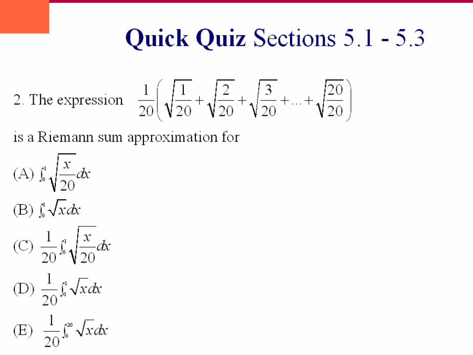
5.3 Definite Integrals and Antiderivatives

Use graphs and your knowledge of area and
x3
0
1
∫ dx = 14
to evaluate the integral.
a) x3
−1
1
∫ dx b) x3 + 3( )0
1
∫ dx
c) x - 2( )3
2
3
∫ dx d) x3
−1
1
∫ dx
d) 1 - x3( )0
1
∫ dx e) x - 1( )3
−1
2
∫ dx
0 13
4
1
4
1
2
3
4−
1
4

Use graphs and your knowledge of area and
x3
0
1
∫ dx = 14
to evaluate the integral.
g) x2
⎛⎝⎜
⎞⎠⎟3
0
2
∫ dx h) x3
−8
8
∫ dx
i) x3 - 1( )0
1
∫ dx j) x3
0
1
∫ dx
01
2
−3
43
4

Page 285 gives rules for working with integrals, the most important of which are:
2. ( ) 0a
af x dx =∫ If the upper and lower limits are equal,
then the integral is zero.
1. ( ) ( )b a
a bf x dx f x dx= −∫ ∫ Reversing the limits
changes the sign.
( ) ( )b b
a ak f x dx k f x dx⋅ =∫ ∫3. Constant multiples can be
moved outside.
→

1.
( ) 0a
af x dx =∫ If the upper and lower limits are equal,
then the integral is zero.2.
( ) ( )b a
a bf x dx f x dx= −∫ ∫ Reversing the limits
changes the sign.
( ) ( )b b
a ak f x dx k f x dx⋅ =∫ ∫3. Constant multiples can be
moved outside.
( ) ( ) ( ) ( )b b b
a a af x g x dx f x dx g x dx+ = +⎡ ⎤⎣ ⎦∫ ∫ ∫4.
Integrals can be added and subtracted.
→

( ) ( ) ( ) ( )b b b
a a af x g x dx f x dx g x dx+ = +⎡ ⎤⎣ ⎦∫ ∫ ∫4.
Integrals can be added and subtracted.
5. ( ) ( ) ( )b c c
a b af x dx f x dx f x dx+ =∫ ∫ ∫
Intervals can be added(or subtracted.)
a b c
( )y f x=
→

Ex: Suppose f and h are continuous functions such that:
f x( )1
9
∫ dx = -1, f x( )7
9
∫ dx =5, h x( )7
9
∫ dx = 4
a) −2 f x( )1
9
∫ dx
b) f x( ) + h(x) ( ) 7
9
∫ dx
c) 2 f x( )−3 h(x)( )7
9
∫ dx
2
9
-2
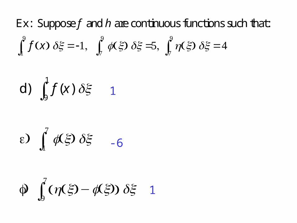
Ex: Suppose f and h are continuous functions such that:
f x( )1
9
∫ dx = -1, f x( )7
9
∫ dx =5, h x( )7
9
∫ dx = 4
d) f (x)9
1
∫ dx
e) f(x)1
7
∫ dx
f) h x( )− f(x)( )9
7
∫ dx
1
-6
1
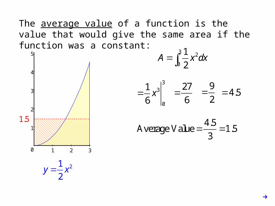
The average value of a function is the value that would give the same area if the function was a constant:
0
1
2
3
4
5
1 2 3
21
2y x=
3 2
0
1
2A x dx=∫
33
0
1
6x=
27
6=
9
2= 4.5=
4.5Average Value 1.5
3= =
1.5
→
Exploration Activity

How long is the average chord of a circle with radius r?
1
-1
-2 2-r r
favg =1
b−ar2 −x2
a
b
∫ dx
favg =1
r−(−r)2 r2 −x2
−r
r
∫ dx
favg =12r
2 r2 −x2
−r
r
∫ dx
favg =12r
2πr2
2 =
πr2

The mean value theorem for definite integrals says that for a continuous function, at some point on the interval the actual value will equal to the average value.
Mean Value Theorem (for definite integrals)
If f is continuous on then at some point c in , [ ],a b [ ],a b
( ) ( )1
b
af c f x dx
b a=
− ∫
π