5 Transformation Between the Celestial and Terrestrial

Systems (16 February 2007)

The coordinate transformation to be used to transform from the terrestrial reference system (TRS)to the celestial reference system (CRS) at the epoch t of the observation can be written as:

[CRS] = Q(t)R(t)W (t) [TRS], (1)

where Q(t), R(t) and W (t) are the transformation matrices arising from the motion of the celestialpole in the celestial system, from the rotation of the Earth around the axis of the pole, and frompolar motion respectively. The frame as realized from the [TRS] by applying the transformationsW (t) and then R(t) will be called “the intermediate reference frame of epoch t.”

5.1 The Framework of IAU 2000 Resolutions

Several resolutions were adopted by the XXIVth General Assembly of the International Astronom-ical Union (Manchester, August 2000) that concern the transformation between the celestial andterrestrial reference systems and are therefore to be implemented in the IERS procedures. Sucha transformation being also required for computing directions of celestial objects in intermediatesystems, the process to transform among these systems consistent with the IAU resolutions is alsoprovided at the end of this chapter.

Resolution B1.3 specifies that the systems of space-time coordinates as defined by IAU ResolutionA4 (1991) for the solar system and the Earth within the framework of General Relativity are nownamed the Barycentric Celestial Reference System (BCRS) and the Geocentric Celestial ReferenceSystem (GCRS) respectively. It also provides a general framework for expressing the metric tensorand defining coordinate transformations at the first post-Newtonian level.

Resolution B1.6 recommends that, beginning on 1 January 2003, the IAU 1976 precession modeland IAU 1980 theory of nutation be replaced by the precession-nutation model IAU 2000A (MHB2000 based on the transfer functions of Mathews et al., (2002)) for those who need a model at the0.2 mas level, or its shorter version IAU 2000B for those who need a model only at the 1 mas level,together with their associated celestial pole offsets, published in this document.

Resolution B1.7 recommends that the Celestial Intermediate Pole (CIP) be implemented in placeof the Celestial Ephemeris Pole (CEP) on 1 January 2003 and specifies how to implement itsdefinition through its direction at J2000.0 in the GCRS as well as the realization of its motionboth in the GCRS and ITRS. Its definition is an extension of that of the CEP in the high frequencydomain and coincides with that of the CEP in the low frequency domain (Capitaine, 2000).

Resolution B1.8 recommends the use of the “non-rotating origin” (NRO) (Guinot, 1979) both in theGCRS and the ITRS and these origins are designated as the Celestial Intermediate Origin (CIO)and the Terrestrial Intermediate Origin (TIO). The “Earth Rotation Angle” is defined as the anglemeasured along the equator of the CIP between the CIO and the TIO. This resolution recommendsthat UT1 be linearly proportional to the Earth Rotation Angle and that the transformation betweenthe ITRS and GCRS be specified by the position of the CIP in the GCRS, the position of the CIPin the ITRS, and the Earth Rotation Angle. It is recommended that the IERS takes steps toimplement this by 1 January 2003 and that the IERS will continue to provide users with data andalgorithms for the conventional transformation.

Following the recommendations above, this chapter of the IERS Conventions provides the expres-sions for the implementation of the IAU resolutions using the new transformation which is describedin Resolution B1.8. It also provides the expressions which are necessary to be compatible withthe resolutions when using the conventional transformation. Numerical values contained in thischapter have been slightly revised from earlier provisional values to ensure continuity of the IERSproducts. Fortran subroutines implementing the transformations are described towards the end ofthe chapter. More detailed explanations about the relevant concepts, software and IERS productscan be found in IERS Technical Note 29 (Capitaine et al., 2002).

1

5.2 Implementation of IAU 2000 Resolutions

In order to follow Resolution B1.3, the celestial reference system, which is designated here CRS,must correspond to the geocentric space coordinates of the GCRS. IAU Resolution A4 (1991)specified that the relative orientation of barycentric and geocentric spatial axes in BCRS andGCRS are without any time dependent rotation. This requires that the geodesic precession andnutation be taken into account in the precession-nutation model.

Concerning the time coordinates, IAU Resolution A4 (1991) defined TCB and TCG of the BCRSand GCRS respectively, as well as another time coordinate in the GCRS, Terrestrial Time (TT),which is the theoretical counterpart of the realized time scale TAI + 32.184 s and has been re-defined by IAU resolution B1.9 (2000). See Chapter 10 for the relationships between these timescales.

The parameter t, used in the following expressions, is defined by

t = (TT − 2000 January 1d 12h TT) in days/36525. (2)

This definition is consistent with IAU Resolution C7 (1994) which recommends that the epochJ2000.0 be defined at the geocenter and at the date 2000 January 1.5 TT = Julian Date 2451545.0TT.

In order to follow Resolution B1.6, the precession-nutation quantities to be used in the transfor-mation matrix Q(t) must be based on the precession-nutation model IAU 2000A or IAU 2000Bdepending on the required precision. In order to follow Resolution B1.7, the realized celestial polemust be the CIP. This requires an offset at epoch in the conventional model for precession-nutationas well as diurnal and higher frequency variations in the Earth’s orientation. According to thisresolution, the direction of the CIP at J2000.0 has to be offset from the pole of the GCRS in amanner consistent with the IAU 2000A precession-nutation model. The motion of the CIP in theGCRS is realized by the IAU 2000 model for precession and forced nutation for periods greaterthan two days plus additional time-dependent corrections provided by the IERS through appro-priate astro-geodetic observations. The motion of the CIP in the ITRS is provided by the IERSthrough astro-geodetic observations and models including variations with frequencies outside theretrograde diurnal band.

The realization of the CIP thus requires that the IERS monitor the observed differences (reportedas “celestial pole offsets”) with respect to the conventional celestial position of the CIP in the GCRSbased on the IAU 2000 precession-nutation model together with its observed offset at epoch. Italso requires that the motion of the CIP in the TRS be provided by the IERS by observationstaking into account a predictable part specified by a model including the terrestrial motion ofthe pole corresponding to the forced nutations with periods less than two days (in the GCRS)as well as the tidal variations in polar motion. Two equivalent procedures were given in theIERS Conventions (McCarthy, 1996) for the coordinate transformation from the TRS to the CRS.The classical procedure, which was described in detail as option 1, makes use of the equinox forrealizing the intermediate reference frame of date t. It uses apparent Greenwich Sidereal Time(GST) in the transformation matrix R(t) and the classical precession and nutation parameters inthe transformation matrix Q(t).

The second procedure, which was described in detail as option 2, makes use of the “non-rotatingorigin” to realize the intermediate reference frame of date t. It uses the “Earth Rotation Angle,”originally referred to as “stellar angle” in the transformation matrix R(t), and the two coordinatesof the celestial pole in the CRS (Capitaine, 1990) in the transformation matrix Q(t).

Resolutions B1.3, B1.6 and B1.7 can be implemented in any of these procedures if the requirementsdescribed above are followed for the space-time coordinates in the geocentric celestial system, forthe precession and nutation model on which are based the precession and nutation quantities usedin the transformation matrix Q(t) and for the polar motion used in the transformation matrixW (t).

On the other hand, only the second procedure can be in agreement with Resolution B1.8, whichrequires the use of the “non-rotating origin” in both the CRS and the TRS as well as the position

2

of the CIP in the GCRS and in the ITRS. However, the IERS must also provide users with dataand algorithms for the conventional transformation; this implies that the expression of GreenwichSidereal Time (GST) has to be consistent with the new procedure.

The following sections give the details of this procedure and the standard expressions necessary toobtain the numerical values of the relevant parameters at the date of the observation.

5.3 Coordinate Transformation consistent with the IAU 2000 Resolutions

In the following, R1, R2 and R3 denote rotation matrices with positive angle about the axes 1,2 and 3 of the coordinate frame. The position of the CIP both in the TRS and CRS is providedby the x and y components of the CIP unit vector. These components are called “coordinates” inthe following and their numerical expressions are multiplied by the factor 1296000′′/2π in order toprovide in arcseconds the value of the corresponding “angles” with respect to the polar axis of thereference system.

The coordinate transformation (1) from the TRS to the CRS corresponding to the procedureconsistent with Resolution B1.8 is expressed in terms of the three fundamental components asgiven below (Capitaine, 1990)

W (t) = R3(−s′) · R2(xp) · R1(yp), (3)

xp and yp being the “polar coordinates” of the Celestial Intermediate Pole (CIP) in the TRS and s′

being a quantity which provides the position of the TIO on the equator of the CIP correspondingto the kinematical definition of the NRO in the ITRS when the CIP is moving with respect to theITRS due to polar motion. The expression of s′ as a function of the coordinates xp and yp is:

s′(t) = (1/2)∫ t

t0

(xpyp − xpyp) dt. (4)

The use of the quantity s′, which was neglected in the classical form prior to 1 January 2003, isnecessary to provide an exact realization of the “instantaneous prime meridian.”

R(t) = R3(−θ), (5)

θ being the Earth Rotation Angle between the CIO and the TIO at date t on the equator of theCIP, which provides a rigorous definition of the sidereal rotation of the Earth.

Q(t) = R3(−E) ·R2(−d) ·R3(E) · R3(s), (6)

E and d being such that the coordinates of the CIP in the CRS are:

X = sin d cosE, Y = sin d sinE, Z = cos d, (7)

and s being a quantity which provides the position of the CIO on the equator of the CIP corre-sponding to the kinematical definition of the NRO in the GCRS when the CIP is moving withrespect to the GCRS, between the reference epoch and the epoch t due to precession and nutation.Its expression as a function of the coordinates X and Y is (Capitaine et al., 2000)

s(t) = −∫ t

t0

X(t)Y (t) − Y (t)X(t)1 + Z(t)

dt− (σ0N0 − Σ0N0), (8)

where σ0 and Σ0 are the positions of the CIO at J2000.0 and the x-origin of the GCRS respectivelyandN0 is the ascending node of the equator at J2000.0 in the equator of the GCRS. Or equivalently,within 1 microarcsecond over one century

s(t) = −12[X(t)Y (t) −X(t0)Y (t0)] +

∫ t

t0

X(t)Y (t)dt− (σ0N0 − Σ0N0). (9)

3

The arbitrary constant σ0N0 − Σ0N0, which had been conventionally chosen to be zero in previ-ous references (e.g. Capitaine et al., 2000), is now chosen to ensure continuity with the classicalprocedure on 1 January 2003 (see expression (36)).

Q(t) can be given in an equivalent form directly involving X and Y as

Q(t) =

⎛⎝ 1 − aX2 −aXY X

−aXY 1 − aY 2 Y−X −Y 1 − a(X2 + Y 2)

⎞⎠ ·R3(s), (10)

with a = 1/(1+cosd), which can also be written, with an accuracy of 1 μas, as a = 1/2+1/8(X2+Y 2). Such an expression of the transformation (1) leads to very simple expressions of the partialderivatives of observables with respect to the terrestrial coordinates of the CIP, UT1, and celestialcoordinates of the CIP.

5.4 Parameters to be used in the Transformation

5.4.1 Schematic Representation of the Motion of the CIP

According to Resolution B1.7, the CIP is an intermediate pole separating, by convention, themotion of the pole of the TRS in the CRS into two parts:

• the celestial motion of the CIP (precession/nutation), including all the terms with periodsgreater than 2 days in the CRS (i.e. frequencies between −0.5 counts per sidereal day (cpsd)and +0.5 cpsd),

• the terrestrial motion of the CIP (polar motion), including all the terms outside the retrogradediurnal band in the TRS (i.e. frequencies lower than −1.5 cpsd or greater than −0.5 cpsd).

frequency in TRS−3.5 −2.5 −1.5 −0.5 +0.5 +1.5 +2.5 (cpsd)

polar motion polar motion

frequency in CRS−2.5 −1.5 −0.5 +0.5 +1.5 +2.5 +3.5 (cpsd)

nutation

5.4.2 Motion of the CIP in the ITRS

The standard pole coordinates to be used for the parameters xp and yp, if not estimated fromthe observations, are those published by the IERS with additional components to account for theeffects of ocean tides and for nutation terms with periods less than two days.

(xp, yp) = (x, y)IERS + (Δx,Δy)tidal + (Δx,Δy)nutation,

where (x, y)IERS are pole coordinates provided by the IERS, (Δx,Δy)tidal are the tidal compo-nents, and (Δx,Δy)nutation are the nutation components. The corrections for these variations aredescribed below.

Corrections (Δx,Δy)tidal for the diurnal and sub-diurnal variations in polar motion caused byocean tides can be computed using a routine available on the website of the IERS Conventions (seeChapter 8). Table 8.2 (from Ch. Bizouard), based on this routine, provides the amplitudes andarguments of these variations for the 71 tidal constituents considered in the model. These subdailyvariations are not part of the polar motion values reported to and distributed by the IERS andare therefore to be added after interpolation.

Recent models for rigid Earth nutation (Souchay and Kinoshita, 1997; Bretagnon et al., 1997;Folgueira et al., 1998a; Folgueira et al., 1998b; Souchay et al., 1999; Roosbeek, 1999; Bizouardet al., 2000; Bizouard et al., 2001) include prograde diurnal and prograde semidiurnal terms withrespect to the GCRS with amplitudes up to ∼ 15 μas in Δψ sin ε0 and Δε. The semidiurnalterms in nutation have also been provided both for rigid and nonrigid Earth models based onHamiltonian formalism (Getino et al., 2001, Escapa et al., 2002a and b). In order to realize the

4

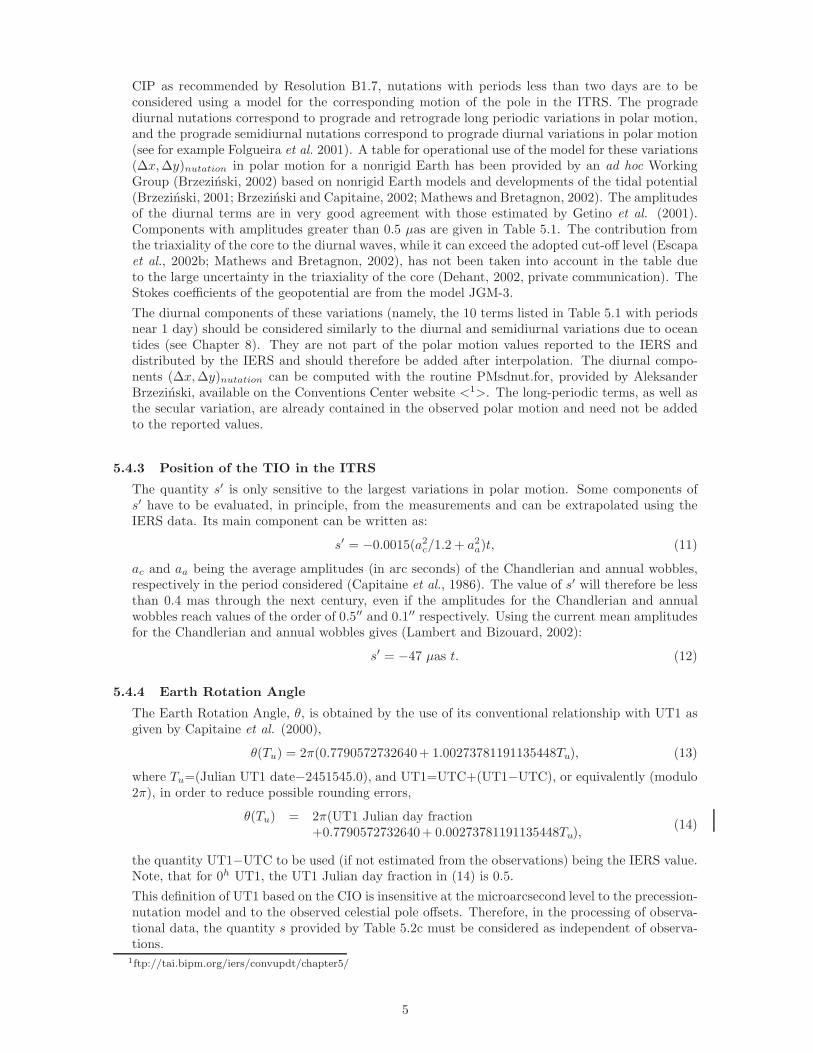
CIP as recommended by Resolution B1.7, nutations with periods less than two days are to beconsidered using a model for the corresponding motion of the pole in the ITRS. The progradediurnal nutations correspond to prograde and retrograde long periodic variations in polar motion,and the prograde semidiurnal nutations correspond to prograde diurnal variations in polar motion(see for example Folgueira et al. 2001). A table for operational use of the model for these variations(Δx,Δy)nutation in polar motion for a nonrigid Earth has been provided by an ad hoc WorkingGroup (Brzezinski, 2002) based on nonrigid Earth models and developments of the tidal potential(Brzezinski, 2001; Brzezinski and Capitaine, 2002; Mathews and Bretagnon, 2002). The amplitudesof the diurnal terms are in very good agreement with those estimated by Getino et al. (2001).Components with amplitudes greater than 0.5 μas are given in Table 5.1. The contribution fromthe triaxiality of the core to the diurnal waves, while it can exceed the adopted cut-off level (Escapaet al., 2002b; Mathews and Bretagnon, 2002), has not been taken into account in the table dueto the large uncertainty in the triaxiality of the core (Dehant, 2002, private communication). TheStokes coefficients of the geopotential are from the model JGM-3.

The diurnal components of these variations (namely, the 10 terms listed in Table 5.1 with periodsnear 1 day) should be considered similarly to the diurnal and semidiurnal variations due to oceantides (see Chapter 8). They are not part of the polar motion values reported to the IERS anddistributed by the IERS and should therefore be added after interpolation. The diurnal compo-nents (Δx,Δy)nutation can be computed with the routine PMsdnut.for, provided by AleksanderBrzezinski, available on the Conventions Center website <1>. The long-periodic terms, as well asthe secular variation, are already contained in the observed polar motion and need not be addedto the reported values.

5.4.3 Position of the TIO in the ITRS

The quantity s′ is only sensitive to the largest variations in polar motion. Some components ofs′ have to be evaluated, in principle, from the measurements and can be extrapolated using theIERS data. Its main component can be written as:

s′ = −0.0015(a2c/1.2 + a2

a)t, (11)

ac and aa being the average amplitudes (in arc seconds) of the Chandlerian and annual wobbles,respectively in the period considered (Capitaine et al., 1986). The value of s′ will therefore be lessthan 0.4 mas through the next century, even if the amplitudes for the Chandlerian and annualwobbles reach values of the order of 0.5′′ and 0.1′′ respectively. Using the current mean amplitudesfor the Chandlerian and annual wobbles gives (Lambert and Bizouard, 2002):

s′ = −47 μas t. (12)

5.4.4 Earth Rotation Angle

The Earth Rotation Angle, θ, is obtained by the use of its conventional relationship with UT1 asgiven by Capitaine et al. (2000),

θ(Tu) = 2π(0.7790572732640+ 1.00273781191135448Tu), (13)

where Tu=(Julian UT1 date−2451545.0), and UT1=UTC+(UT1−UTC), or equivalently (modulo2π), in order to reduce possible rounding errors,

θ(Tu) = 2π(UT1 Julian day fraction+0.7790572732640+ 0.00273781191135448Tu),

(14)

the quantity UT1−UTC to be used (if not estimated from the observations) being the IERS value.Note, that for 0h UT1, the UT1 Julian day fraction in (14) is 0.5.This definition of UT1 based on the CIO is insensitive at the microarcsecond level to the precession-nutation model and to the observed celestial pole offsets. Therefore, in the processing of observa-tional data, the quantity s provided by Table 5.2c must be considered as independent of observa-tions.

1ftp://tai.bipm.org/iers/convupdt/chapter5/

5

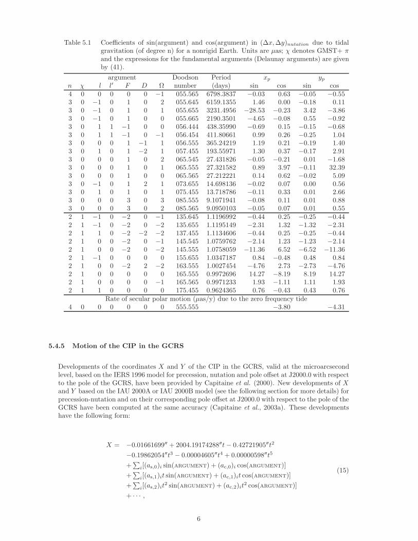
Table 5.1 Coefficients of sin(argument) and cos(argument) in (Δx,Δy)nutation due to tidalgravitation (of degree n) for a nonrigid Earth. Units are μas; χ denotes GMST+ πand the expressions for the fundamental arguments (Delaunay arguments) are givenby (41).

argument Doodson Period xp yp

n χ l l′ F D Ω number (days) sin cos sin cos4 0 0 0 0 0 −1 055.565 6798.3837 −0.03 0.63 −0.05 −0.553 0 −1 0 1 0 2 055.645 6159.1355 1.46 0.00 −0.18 0.113 0 −1 0 1 0 1 055.655 3231.4956 −28.53 −0.23 3.42 −3.863 0 −1 0 1 0 0 055.665 2190.3501 −4.65 −0.08 0.55 −0.923 0 1 1 −1 0 0 056.444 438.35990 −0.69 0.15 −0.15 −0.683 0 1 1 −1 0 −1 056.454 411.80661 0.99 0.26 −0.25 1.043 0 0 0 1 −1 1 056.555 365.24219 1.19 0.21 −0.19 1.403 0 1 0 1 −2 1 057.455 193.55971 1.30 0.37 −0.17 2.913 0 0 0 1 0 2 065.545 27.431826 −0.05 −0.21 0.01 −1.683 0 0 0 1 0 1 065.555 27.321582 0.89 3.97 −0.11 32.393 0 0 0 1 0 0 065.565 27.212221 0.14 0.62 −0.02 5.093 0 −1 0 1 2 1 073.655 14.698136 −0.02 0.07 0.00 0.563 0 1 0 1 0 1 075.455 13.718786 −0.11 0.33 0.01 2.663 0 0 0 3 0 3 085.555 9.1071941 −0.08 0.11 0.01 0.883 0 0 0 3 0 2 085.565 9.0950103 −0.05 0.07 0.01 0.552 1 −1 0 −2 0 −1 135.645 1.1196992 −0.44 0.25 −0.25 −0.442 1 −1 0 −2 0 −2 135.655 1.1195149 −2.31 1.32 −1.32 −2.312 1 1 0 −2 −2 −2 137.455 1.1134606 −0.44 0.25 −0.25 −0.442 1 0 0 −2 0 −1 145.545 1.0759762 −2.14 1.23 −1.23 −2.142 1 0 0 −2 0 −2 145.555 1.0758059 −11.36 6.52 −6.52 −11.362 1 −1 0 0 0 0 155.655 1.0347187 0.84 −0.48 0.48 0.842 1 0 0 −2 2 −2 163.555 1.0027454 −4.76 2.73 −2.73 −4.762 1 0 0 0 0 0 165.555 0.9972696 14.27 −8.19 8.19 14.272 1 0 0 0 0 −1 165.565 0.9971233 1.93 −1.11 1.11 1.932 1 1 0 0 0 0 175.455 0.9624365 0.76 −0.43 0.43 0.76

Rate of secular polar motion (μas/y) due to the zero frequency tide4 0 0 0 0 0 0 555.555 −3.80 −4.31

5.4.5 Motion of the CIP in the GCRS

Developments of the coordinates X and Y of the CIP in the GCRS, valid at the microarcsecondlevel, based on the IERS 1996 model for precession, nutation and pole offset at J2000.0 with respectto the pole of the GCRS, have been provided by Capitaine et al. (2000). New developments of Xand Y based on the IAU 2000A or IAU 2000B model (see the following section for more details) forprecession-nutation and on their corresponding pole offset at J2000.0 with respect to the pole of theGCRS have been computed at the same accuracy (Capitaine et al., 2003a). These developmentshave the following form:

X = −0.01661699′′ + 2004.19174288′′t− 0.42721905′′t2

−0.19862054′′t3 − 0.00004605′′t4 + 0.00000598′′t5

+∑

i[(as,0)i sin(ARGUMENT) + (ac,0)i cos(ARGUMENT)]+

∑i[(as,1)it sin(ARGUMENT) + (ac,1)it cos(ARGUMENT)]

+∑

i[(as,2)it2 sin(ARGUMENT) + (ac,2)it

2 cos(ARGUMENT)]+ · · · ,

(15)

6

Y = −0.00695078′′ − 0.02538199′′t− 22.40725099′′t2

+0.00184228′′t3 + 0.00111306′′t4 + 0.00000099′′t5

+∑

i[(bc,0)i cos(ARGUMENT) + (bs,0)i sin(ARGUMENT)]+

∑i[(bc,1)it cos(ARGUMENT) + (bs,1)i t sin(ARGUMENT)]

+∑

i[(bc,2)it2 cos(ARGUMENT) + (bs,2)it

2 sin(ARGUMENT)]+ · · · ,

(16)

the parameter t being given by expression (2) and ARGUMENT being a function of the fundamentalarguments of the nutation theory whose expressions are given by (41) for the lunisolar ones and(42) for the planetary ones.

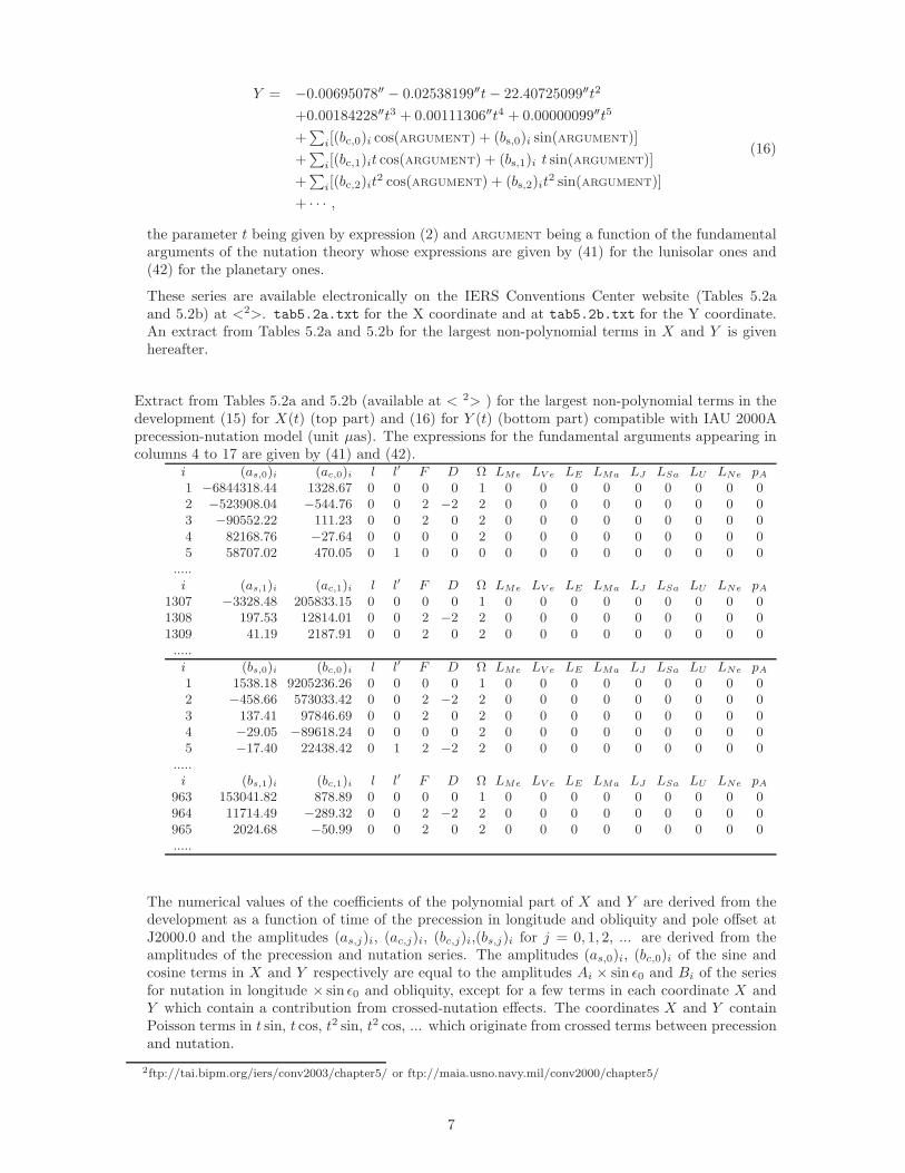
These series are available electronically on the IERS Conventions Center website (Tables 5.2aand 5.2b) at <2>. tab5.2a.txt for the X coordinate and at tab5.2b.txt for the Y coordinate.An extract from Tables 5.2a and 5.2b for the largest non-polynomial terms in X and Y is givenhereafter.

Extract from Tables 5.2a and 5.2b (available at < 2> ) for the largest non-polynomial terms in thedevelopment (15) for X(t) (top part) and (16) for Y (t) (bottom part) compatible with IAU 2000Aprecession-nutation model (unit μas). The expressions for the fundamental arguments appearing incolumns 4 to 17 are given by (41) and (42).

i (as,0)i (ac,0)i l l′ F D Ω LMe LV e LE LMa LJ LSa LU LNe pA

1 −6844318.44 1328.67 0 0 0 0 1 0 0 0 0 0 0 0 0 02 −523908.04 −544.76 0 0 2 −2 2 0 0 0 0 0 0 0 0 03 −90552.22 111.23 0 0 2 0 2 0 0 0 0 0 0 0 0 04 82168.76 −27.64 0 0 0 0 2 0 0 0 0 0 0 0 0 05 58707.02 470.05 0 1 0 0 0 0 0 0 0 0 0 0 0 0

.....i (as,1)i (ac,1)i l l′ F D Ω LMe LV e LE LMa LJ LSa LU LNe pA

1307 −3328.48 205833.15 0 0 0 0 1 0 0 0 0 0 0 0 0 01308 197.53 12814.01 0 0 2 −2 2 0 0 0 0 0 0 0 0 01309 41.19 2187.91 0 0 2 0 2 0 0 0 0 0 0 0 0 0.....

i (bs,0)i (bc,0)i l l′ F D Ω LMe LV e LE LMa LJ LSa LU LNe pA

1 1538.18 9205236.26 0 0 0 0 1 0 0 0 0 0 0 0 0 02 −458.66 573033.42 0 0 2 −2 2 0 0 0 0 0 0 0 0 03 137.41 97846.69 0 0 2 0 2 0 0 0 0 0 0 0 0 04 −29.05 −89618.24 0 0 0 0 2 0 0 0 0 0 0 0 0 05 −17.40 22438.42 0 1 2 −2 2 0 0 0 0 0 0 0 0 0

.....i (bs,1)i (bc,1)i l l′ F D Ω LMe LV e LE LMa LJ LSa LU LNe pA

963 153041.82 878.89 0 0 0 0 1 0 0 0 0 0 0 0 0 0964 11714.49 −289.32 0 0 2 −2 2 0 0 0 0 0 0 0 0 0965 2024.68 −50.99 0 0 2 0 2 0 0 0 0 0 0 0 0 0.....

The numerical values of the coefficients of the polynomial part of X and Y are derived from thedevelopment as a function of time of the precession in longitude and obliquity and pole offset atJ2000.0 and the amplitudes (as,j)i, (ac,j)i, (bc,j)i,(bs,j)i for j = 0, 1, 2, ... are derived from theamplitudes of the precession and nutation series. The amplitudes (as,0)i, (bc,0)i of the sine andcosine terms in X and Y respectively are equal to the amplitudes Ai × sin ε0 and Bi of the seriesfor nutation in longitude × sin ε0 and obliquity, except for a few terms in each coordinate X andY which contain a contribution from crossed-nutation effects. The coordinates X and Y containPoisson terms in t sin, t cos, t2 sin, t2 cos, ... which originate from crossed terms between precessionand nutation.

2ftp://tai.bipm.org/iers/conv2003/chapter5/ or ftp://maia.usno.navy.mil/conv2000/chapter5/

7

The contributions (in μas) to expressions (15) and (16) from the frame biases are

dX = −16617.0− 1.6 t2 + 0.7 cosΩ,dY = −6819.2− 141.9 t+ 0.5 sin Ω, (17)

the first term in each coordinate being the contribution from the celestial pole offset at J2000.0 andthe following ones from the equinox offset at J2000.0 also called “frame bias in right ascension.”

The celestial coordinates of the CIP, X and Y , can also be obtained at each time t as a functionof the precession and nutation quantities provided by the IAU 2000 precession-nutation model.The developments to be used for the precession quantities and for the nutation angles referredto the ecliptic of date are described in the following section and a subroutine is available for thecomputation.

The relationships between the coordinates X and Y and the precession-nutation quantities are(Capitaine, 1990):

X = X + ξ0 − dα0 Y ,Y = Y + η0 + dα0 X,

(18)

where ξ0 and η0 are the celestial pole offsets at the basic epoch J2000.0 and dα0 the right ascensionof the mean equinox of J2000.0 in the CRS. (See the numbers provided below in (19) and (28) forthese quantities.)

The mean equinox of J2000.0 to be considered is not the “rotational dynamical mean equinoxof J2000.0” as used in the past, but the “inertial dynamical mean equinox of J2000.0” to whichthe recent numerical or analytical solutions refer. The latter is associated with the ecliptic in theinertial sense, which is the plane perpendicular to the vector angular momentum of the orbitalmotion of the Earth-Moon barycenter as computed from the velocity of the barycenter relative toan inertial frame. The rotational equinox is associated with the ecliptic in the rotational sense,which is perpendicular to the vector angular momentum computed from the velocity referred tothe rotating orbital plane of the Earth-Moon barycenter. (The difference between the two angularmomenta is the angular momentum associated with the rotation of the orbital plane.) See Standish(1981) for more details. The numerical value for dα0 as derived from Chapront et al. (2002) to beused in expression (18) is

dα0 = (−0.01460± 0.00050)′′. (19)

Quantities X and Y are given by:

X = sinω sinψ,Y = − sin ε0 cosω + cos ε0 sinω cosψ (20)

where ε0 (= 84381.448′′) is the obliquity of the ecliptic at J2000.0, ω is the inclination of the trueequator of date on the fixed ecliptic of epoch and ψ is the longitude, on the ecliptic of epoch, ofthe node of the true equator of date on the fixed ecliptic of epoch; these quantities are such that

ω = ωA + Δε1; ψ = ψA + Δψ1, (21)

where ψA and ωA are the precession quantities in longitude and obliquity (Lieske et al., 1977)referred to the ecliptic of epoch and Δψ1, Δε1 are the nutation angles in longitude and obliquityreferred to the ecliptic of epoch. (See the numerical developments provided for the precessionquantities in (30) and (31).) Δψ1, Δε1 can be obtained from the nutation angles Δψ, Δε inlongitude and obliquity referred to the ecliptic of date. The following formulation from Aoki andKinoshita (1983) has been verified to provide an accuracy better than one microarcsecond afterone century:

Δψ1 sinωA = Δψ sin εA cosχA − Δε sinχA,Δε1 = Δψ sin εA sinχA + Δε cosχA,

(22)

ωA and εA being the precession quantities in obliquity referred to the ecliptic of epoch and theecliptic of date respectively and χA the planetary precession along the equator (Lieske et al., 1977).

8

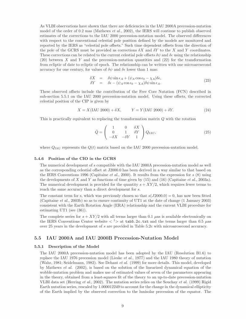
As VLBI observations have shown that there are deficiencies in the IAU 2000A precession-nutationmodel of the order of 0.2 mas (Mathews et al., 2002), the IERS will continue to publish observedestimates of the corrections to the IAU 2000 precession-nutation model. The observed differenceswith respect to the conventional celestial pole position defined by the models are monitored andreported by the IERS as “celestial pole offsets.” Such time dependent offsets from the direction ofthe pole of the GCRS must be provided as corrections δX and δY to the X and Y coordinates.These corrections can be related to the current celestial pole offsets δψ and δε using the relationship(20) between X and Y and the precession-nutation quantities and (22) for the transformationfrom ecliptic of date to ecliptic of epoch. The relationship can be written with one microarcsecondaccuracy for one century, for values of δψ and δε lower than 1 mas:

δX = δψ sin εA + (ψA cos ε0 − χA)δε,δY = δε− (ψA cos ε0 − χA)δψ sin εA.

(23)

These observed offsets include the contribution of the Free Core Nutation (FCN) described insub-section 5.5.1 on the IAU 2000 precession-nutation model. Using these offsets, the correctedcelestial position of the CIP is given by

X = X(IAU 2000) + δX, Y = Y (IAU 2000) + δY. (24)

This is practically equivalent to replacing the transformation matrix Q with the rotation

Q =

⎛⎝ 1 0 δX

0 1 δY−δX −δY 1

⎞⎠QIAU, (25)

where QIAU represents the Q(t) matrix based on the IAU 2000 precession-nutation model.

5.4.6 Position of the CIO in the GCRS

The numerical development of s compatible with the IAU 2000A precession-nutation model as wellas the corresponding celestial offset at J2000.0 has been derived in a way similar to that based onthe IERS Conventions 1996 (Capitaine et al., 2000). It results from the expression for s (8) usingthe developments of X and Y as functions of time given by (15) and (16) (Capitaine et al., 2003a).The numerical development is provided for the quantity s+XY/2, which requires fewer terms toreach the same accuracy than a direct development for s.

The constant term for s, which was previously chosen so that s(J2000.0) = 0, has now been fitted(Capitaine et al., 2003b) so as to ensure continuity of UT1 at the date of change (1 January 2003)consistent with the Earth Rotation Angle (ERA) relationship and the current VLBI procedure forestimating UT1 (see (36)).

The complete series for s+XY/2 with all terms larger than 0.1 μas is available electronically onthe IERS Conventions Center website < 1> at tab5.2c.txt and the terms larger than 0.5 μasover 25 years in the development of s are provided in Table 5.2c with microarcsecond accuracy.

5.5 IAU 2000A and IAU 2000B Precession-Nutation Model

5.5.1 Description of the Model

The IAU 2000A precession-nutation model has been adopted by the IAU (Resolution B1.6) toreplace the IAU 1976 precession model (Lieske et al., 1977) and the IAU 1980 theory of nutation(Wahr, 1981; Seidelmann, 1982). See Dehant et al. (1999) for more details. This model, developedby Mathews et al. (2002), is based on the solution of the linearized dynamical equation of thewobble-nutation problem and makes use of estimated values of seven of the parameters appearingin the theory, obtained from a least-squares fit of the theory to an up-to-date precession-nutationVLBI data set (Herring et al., 2002). The nutation series relies on the Souchay et al. (1999) RigidEarth nutation series, rescaled by 1.000012249 to account for the change in the dynamical ellipticityof the Earth implied by the observed correction to the lunisolar precession of the equator. The

9

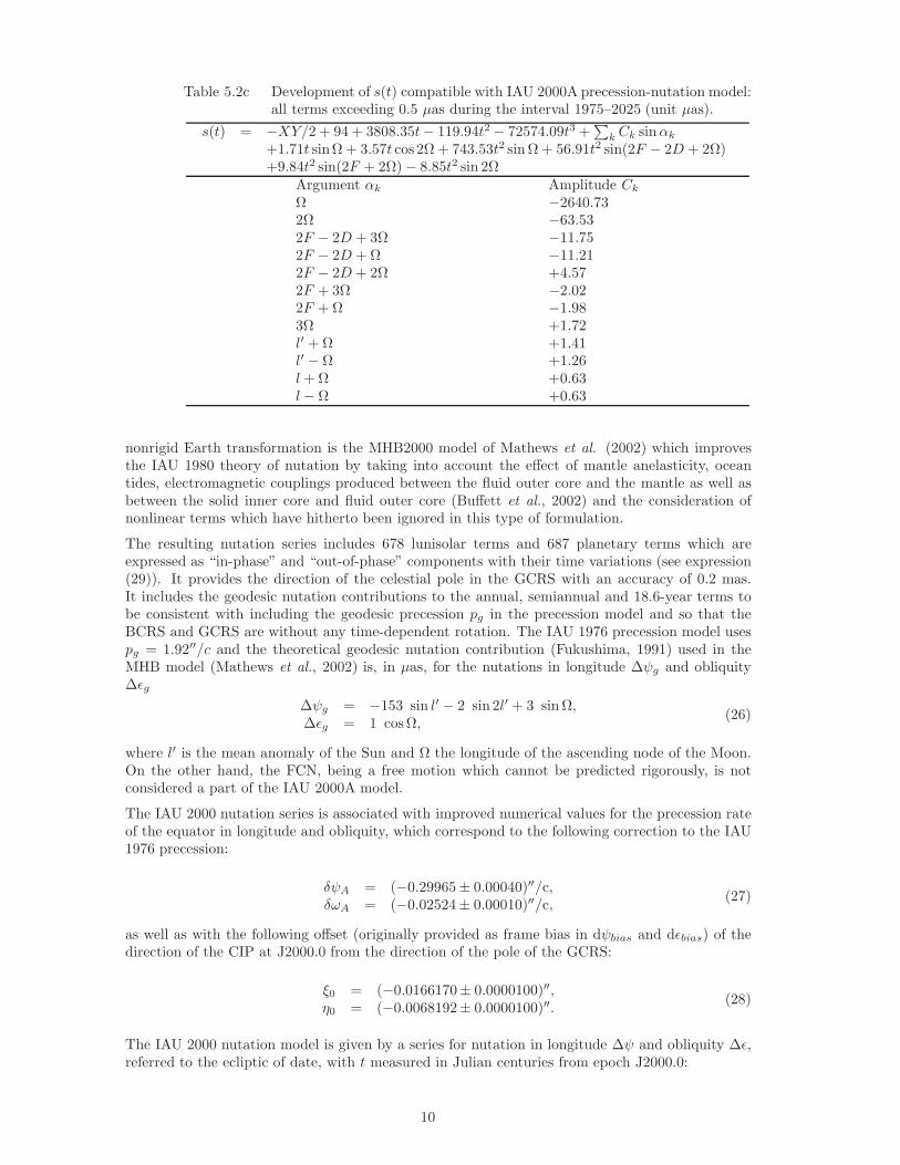
Table 5.2c Development of s(t) compatible with IAU 2000A precession-nutation model:all terms exceeding 0.5 μas during the interval 1975–2025 (unit μas).

s(t) = −XY/2 + 94 + 3808.35t− 119.94t2 − 72574.09t3 +∑

k Ck sinαk

+1.71t sinΩ + 3.57t cos 2Ω + 743.53t2 sin Ω + 56.91t2 sin(2F − 2D + 2Ω)+9.84t2 sin(2F + 2Ω) − 8.85t2 sin 2Ω

Argument αk Amplitude Ck

Ω −2640.732Ω −63.532F − 2D + 3Ω −11.752F − 2D + Ω −11.212F − 2D + 2Ω +4.572F + 3Ω −2.022F + Ω −1.983Ω +1.72l′ + Ω +1.41l′ − Ω +1.26l+ Ω +0.63l− Ω +0.63

nonrigid Earth transformation is the MHB2000 model of Mathews et al. (2002) which improvesthe IAU 1980 theory of nutation by taking into account the effect of mantle anelasticity, oceantides, electromagnetic couplings produced between the fluid outer core and the mantle as well asbetween the solid inner core and fluid outer core (Buffett et al., 2002) and the consideration ofnonlinear terms which have hitherto been ignored in this type of formulation.

The resulting nutation series includes 678 lunisolar terms and 687 planetary terms which areexpressed as “in-phase” and “out-of-phase” components with their time variations (see expression(29)). It provides the direction of the celestial pole in the GCRS with an accuracy of 0.2 mas.It includes the geodesic nutation contributions to the annual, semiannual and 18.6-year terms tobe consistent with including the geodesic precession pg in the precession model and so that theBCRS and GCRS are without any time-dependent rotation. The IAU 1976 precession model usespg = 1.92′′/c and the theoretical geodesic nutation contribution (Fukushima, 1991) used in theMHB model (Mathews et al., 2002) is, in μas, for the nutations in longitude Δψg and obliquityΔεg

Δψg = −153 sin l′ − 2 sin 2l′ + 3 sin Ω,Δεg = 1 cosΩ, (26)

where l′ is the mean anomaly of the Sun and Ω the longitude of the ascending node of the Moon.On the other hand, the FCN, being a free motion which cannot be predicted rigorously, is notconsidered a part of the IAU 2000A model.

The IAU 2000 nutation series is associated with improved numerical values for the precession rateof the equator in longitude and obliquity, which correspond to the following correction to the IAU1976 precession:

δψA = (−0.29965± 0.00040)′′/c,δωA = (−0.02524± 0.00010)′′/c, (27)

as well as with the following offset (originally provided as frame bias in dψbias and dεbias) of thedirection of the CIP at J2000.0 from the direction of the pole of the GCRS:

ξ0 = (−0.0166170± 0.0000100)′′,η0 = (−0.0068192± 0.0000100)′′. (28)

The IAU 2000 nutation model is given by a series for nutation in longitude Δψ and obliquity Δε,referred to the ecliptic of date, with t measured in Julian centuries from epoch J2000.0:

10

Δψ =∑N

i=1(Ai +A′it) sin(ARGUMENT) + (A′′

i +A′′′i t) cos(ARGUMENT),

Δε =∑N

i=1(Bi +B′it) cos(ARGUMENT) + (B′′

i + B′′′i t) sin(ARGUMENT).

(29)

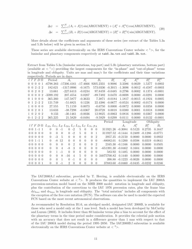
More details about the coefficients and arguments of these series (see extract of the Tables 5.3aand 5.3b below) will be given in section 5.8.

These series are available electronically on the IERS Conventions Center website < 1>, for thelunisolar and planetary components respectively at tab5.3a.txt and tab5.3b.txt.

Extract from Tables 5.3a (lunisolar nutations, top part) and 5.3b (planetary nutations, bottom part)(available at < 1>) providing the largest components for the “in-phase” and “out-of-phase” termsin longitude and obliquity. Units are mas and mas/c for the coefficients and their time variationsrespectively. Periods are in days.l l′ F D Ω Period Ai A′

i Bi B′i A′′

i A′′′i B′′

i B′′′i

0 0 0 0 1 -6798.383 -17206.4161 -17.4666 9205.2331 0.9086 3.3386 0.0029 1.5377 0.00020 0 2 -2 2 182.621 -1317.0906 -0.1675 573.0336 -0.3015 -1.3696 0.0012 -0.4587 -0.00030 0 2 0 2 13.661 -227.6413 -0.0234 97.8459 -0.0485 0.2796 0.0002 0.1374 -0.00010 0 0 0 2 -3399.192 207.4554 0.0207 -89.7492 0.0470 -0.0698 0.0000 -0.0291 0.00000 1 0 0 0 365.260 147.5877 -0.3633 7.3871 -0.0184 1.1817 -0.0015 -0.1924 0.00050 1 2 -2 2 121.749 -51.6821 0.1226 22.4386 -0.0677 -0.0524 0.0002 -0.0174 0.00001 0 0 0 0 27.555 71.1159 0.0073 -0.6750 0.0000 -0.0872 0.0000 0.0358 0.00000 0 2 0 1 13.633 -38.7298 -0.0367 20.0728 0.0018 0.0380 0.0001 0.0318 0.00001 0 2 0 2 9.133 -30.1461 -0.0036 12.9025 -0.0063 0.0816 0.0000 0.0367 0.00000 -1 2 -2 2 365.225 21.5829 -0.0494 -9.5929 0.0299 0.0111 0.0000 0.0132 -0.0001

Period Longitude Obliquityl l′ F D Ω LMe LV e LE LMa LJ LSa LU LNe pA Ai A′′

i B′′i Bi

0 0 1 -1 1 0 0 -1 0 -2 5 0 0 0 311921.26 -0.3084 0.5123 0.2735 0.16470 0 0 0 0 0 0 0 0 -2 5 0 0 1 311927.52 -0.1444 0.2409 -0.1286 -0.07710 0 0 0 0 0 -3 5 0 0 0 0 0 2 2957.35 -0.2150 0.0000 0.0000 0.09320 0 1 -1 1 0 -8 12 0 0 0 0 0 0 -88082.01 0.1200 0.0598 0.0319 -0.06410 0 0 0 0 0 0 0 0 2 0 0 0 2 2165.30 -0.1166 0.0000 0.0000 0.05050 0 0 0 0 0 0 4 -8 3 0 0 0 0 -651391.30 -0.0462 0.1604 0.0000 0.00000 0 0 0 0 0 1 -1 0 0 0 0 0 0 583.92 0.1485 0.0000 0.0000 0.00000 0 0 0 0 0 0 8 -16 4 5 0 0 0 34075700.82 0.1440 0.0000 0.0000 0.00000 0 0 0 0 0 0 1 0 -1 0 0 0 0 398.88 -0.1223 -0.0026 0.0000 0.00000 0 0 0 1 0 0 -1 2 0 0 0 0 0 37883.60 -0.0460 -0.0435 -0.0232 0.0246

The IAU2000A.f subroutine, provided by T. Herring, is available electronically on the IERSConventions Center website at < 2>. It produces the quantities to implement the IAU 2000Aprecession-nutation model based on the MHB 2000 model: nutation in longitude and obliquity,plus the contribution of the corrections to the IAU 1976 precession rates, plus the frame biasdψbias and dεbias in longitude and obliquity. The “total nutation” includes all components withthe exception of the free core nutation (FCN). The software can also be used to model the expectedFCN based on the most recent astronomical observations.

As recommended by Resolution B1.6, an abridged model, designated IAU 2000B, is available forthose who need a model only at the 1 mas level. Such a model has been developed by McCarthyand Luzum (2003). It includes fewer than 80 lunisolar terms plus a bias to account for the effect ofthe planetary terms in the time period under consideration. It provides the celestial pole motionwith an accuracy that does not result in a difference greater than 1 mas with respect to thatof the IAU 2000A model during the period 1995–2050. The IAU2000B.f subroutine is availableelectronically on the IERS Conventions Center website at < 2>.

11

5.5.2 Precession Developments compatible with the IAU2000 Model

The numerical values for the precession quantities compatible with the IAU 2000 precession-nutation model can be provided by using the developments (30) of Lieske et al. (1977) to whichthe estimated corrections (27) δψA and δωA to the IAU 1976 precession have to be added.

The expressions of Lieske et al. (1977) are

ψA = 5038.7784′′t− 1.07259′′t2 − 0.001147′′t3,ωA = ε0 + 0.05127′′t2 − 0.007726′′t3,εA = ε0 − 46.8150′′t− 0.00059′′t2 + 0.001813′′t3,χA = 10.5526′′t− 2.38064′′t2 − 0.001125′′t3 ,

(30)

and

ζA = 2306.2181′′t+ 0.30188′′t2 + 0.017998′′t3,θA = 2004.3109′′t− 0.42665′′t2 − 0.041833′′t3,zA = 2306.2181′′t+ 1.09468′′t2 + 0.018203′′t3,

(31)

with ε0 = 84381.448′′.

Due to their theoretical bases, the original development of the precession quantities as function oftime can be considered as being expressed in TDB.

The expressions compatible with the IAU 2000A precession and nutation are:

ψA = 5038.47875′′t− 1.07259′′t2 − 0.001147′′t3,ωA = ε0 − 0.02524′′t+ 0.05127′′t2 − 0.007726′′t3,εA = ε0 − 46.84024′′t− 0.00059′′t2 + 0.001813′′t3,χA = 10.5526′′t− 2.38064′′t2 − 0.001125′′t3 ,

(32)

and the following series has been developed (Capitaine et al., 2003c) in order to match the 4-rotation series for precession R1(−ε0) ·R3(ψA) ·R1(ωA) ·R3(−χA), called the “canonical 4-rotationmethod,” to sub-microarcsecond accuracy over 4 centuries:

ζA = 2.5976176′′ + 2306.0809506′′t+ 0.3019015′′t2 + 0.0179663′′t3

−0.0000327′′t4 − 0.0000002′′t5,θA = 2004.1917476′′t− 0.4269353′′t2 − 0.0418251′′t3

−0.0000601′′t4 − 0.0000001′′t5,zA = −2.5976176′′ + 2306.0803226′′t+ 1.0947790′′t2 + 0.0182273′′t3

+0.0000470′′t4 − 0.0000003′′t5.

(33)

Note that the new expression for the quantities ζA and zA include a constant term (with oppositesigns) which originates from the ratio between the precession rate in ωA and in ψA sin ε0.

In practice, TT is used in the above expressions in place of TDB. The largest term in the differenceTDB−TT being 1.7 ms × sin l′, the resulting error in the precession quantity ψA is periodic,with an annual period and an amplitude of 2.7′′ × 10−9, which is significantly under the requiredmicroarcsecond accuracy.

5.6 Procedure to be used for the Transformation consistent with IAU 2000Resolutions

There are several ways to implement the IAU 2000 precession-nutation model, and the precessiondevelopments to be used should be consistent with the procedure being used. The subroutinesavailable for the different procedures are described below.

12

Using the new paradigm, the complete procedure to transform from the GCRS to the ITRS com-patible with the IAU 2000A precession-nutation is based on the expressions provided by (15) and(16) and Tables 5.2 for the positions of the CIP and the CIO in the GCRS. These already containthe proper expressions for the new precession-nutation model and the frame biases. Another pro-cedure can also be used for the computation of the coordinates X and Y of the CIP in the GCRSusing expressions (18) to (22). This must be based on the MHB 2000 nutation series, on offsets atJ2000.0 as well as on precession quantities ψA, ωA, εA, χA, taking into account the corrections tothe IAU 1976 precession rates. (See expressions (32).)

In support of the classical paradigm, the IAU2000A subroutine provides the components of theprecession-nutation model including the contributions of the correction to the IAU 1976 precessionrates for ζA, θZ , zA (see expressions (31)). Expressions (33) give the same angles but taking intoaccount the IAU 2000 corrections.

The recommended option for implementing the IAU 2000A/B model using the classical transfor-mation between the TRS and the GCRS is to follow a rigorous procedure described by Wallace (inCapitaine et al., 2002). This procedure is composed of the classical nutation matrix using the MHB2000 series, the precession matrix including four rotations (R1(−ε0) ·R3(ψA) ·R1(ωA) ·R3(−χA))using the updated developments (32) for these quantities and a separate rotation matrix for theframe bias.

In the case when one elects to continue using the classical expressions based on the IAU 1976precession model and IAU 1980 theory of nutation, one should proceed as in the past as describedin the IERS Conventions 1996 (McCarthy, 1996) and then apply the corrections to the modelprovided by the appropriate IAU 2000A/B software.

5.7 Expression of Greenwich Sidereal Time referred to the CIO

Greenwich Sidereal Time (GST), which refers to the equinox, is related to the “Earth RotationAngle” ERA, denoted by θ, that refers to the Celestial Intermediate Origin (CIO), by the followingrelationship (Aoki and Kinoshita, 1983; Capitaine and Gontier, 1993) at the microarcsecond level:

GST = dT0 + θ +∫ t

t0

˙(ψA + Δψ1) cos(ωA + Δε1)dt− χA + Δψ cos εA − Δψ1 cosωA, (34)

Δψ1, Δε1, given by (22), being the nutation angles in longitude and obliquity referred to theecliptic of epoch and χA, whose development is given in (32), the planetary precession along theequator (i.e. the RA component of the precession of the ecliptic).

This can be written as:

GST = θ(UT1) − EO, (35)

where EO is “the equation of the origins” (according to the recommendations of the IAU WG on“Nomenclature for fundamental astronomy”), defined by:

EO = − dT0 −∫ t

t0

˙(ψA + Δψ1) cos(ωA − Δε1)dt+ χA − Δψ cos εA + Δψ1 cosωA, (36)

providing the CIO right ascension of the equinox along the moving equator, which accounts forthe accumulated precession and nutation in right ascension from J2000.0 to the epoch t, and dT0

is a constant term to be fitted in order to ensure continuity in UT1 at the date of change. Thenumerical expression consistent with the IAU 2000A precession-nutation model has been obtainedusing computations similar to those performed for s and following a procedure, which is describedbelow, to ensure consistency at the microarcsecond level among the transformations as well ascontinuity in UT1 at the date of change (Capitaine et al., 2003b).

13

Table 5.4 Development of EO compatible with IAU 2000A precession-nutation model:all terms exceeding 0.5μas during the interval 1975–2025 (unit μas).

EO = − 0.014506′′ − 4612.15739966′′t− 1.39667721′′t2

+ 0.00009344′′t3 − Δψ cos εA − ∑k C

′k sinαk

Argument αk Amplitude C′k

Ω +2640.962Ω +63.522F − 2D + 3Ω +11.752F − 2D + Ω +11.212F − 2D + 2Ω −4.552F + 3Ω +2.022F + Ω +1.983Ω −1.72l′ + Ω −1.41l′ − Ω −1.26l+ Ω −0.63l− Ω −0.63

The series providing the expression for Greenwich Sidereal Time based on the IAU 2000A precession-nutation model is available on the IERS Conventions Center website < 1> at tab5.4.txt, andthe terms larger than 0.5μas over 25 years in the development of EO are provided in Table 5.4with microarcsecond accuracy.

The C′k coefficients are similar to the Ck coefficients appearing in Table 5.2c providing the develop-

ment for s and are equal to these coefficients up to 1μas. The last term of EO, i.e. −∑k C

′k sinαk, is

the complementary term to be subtracted from the classical “equation of the equinoxes,” Δψ cos εA,to provide the relationship between GST and θ with microarcsecond accuracy. This replaces thetwo complementary terms provided in the IERS Conventions 1996. A secular term similar to thatappearing in the quantity s is included in expression (36). This expression for GST used in theclassical transformation based on the IAU 2000A precession-nutation ensures consistency at themicroarcsecond level after one century among transformations using expressions (14) for θ, (15)and (16) for the celestial coordinates of the CIP and Table 5.2c for s. The numerical values for theconstant term dT0 in GST, which ensures continuity in UT1 at the date of change (1 January 2003),and for the corresponding constant term in s have been found to be

dT0 = + 14506μas ,s0 = + 94μas . (37)

The change in the polynomial part of GST due to the correction in the precession rates (27)corresponds to a change dGMST (see also Williams, 1994) in the current relationship betweenGMST and UT1 (Aoki et al., 1982). Its numerical expression derived from expressions (35) forGST, (13) for θ(UT1), and the polynomial part of EO in Table 5.4, minus the expression forGMST1982(UT1), can be written in microarcseconds as

dGMST = 14506− 274950.12 t+ 117.21 t2 − 0.44 t3 + 18.82 t4. (38)

The new expression for GST clearly distinguishes between θ, which is expressed as a function ofUT1, and the EO (i.e. mainly the accumulated precession-nutation in right ascension), which isexpressed in TDB (or, in practice, TT), in contrast to the GMST1982(UT1) expression, which usedonly UT1. This gives rise to an additional difference in dGMST of (TT−UT1) multiplied by thespeed of precession in right ascension. Using TT−TAI = 32.184 s, this is: [47+1.5(TAI−UT1)]μas,where TAI−UT1 is in seconds. On 1 January 2003, this difference is about 94μas (see Gontier inCapitaine et al., 2002), using the value of 32.3 s for TAI−UT1. This contribution for the effect oftime scales is included in the values for dT0 and s0.

14

5.8 The Fundamental Arguments of Nutation Theory

5.8.1 The Multipliers of the Fundamental Arguments of Nutation Theory

Each of the lunisolar terms in the nutation series is characterized by a set of five integers Nj

which determines the ARGUMENT for the term as a linear combination of the five FundamentalArguments Fj , namely the Delaunay variables (�, �′, F,D,Ω): ARGUMENT =

∑5j=1NjFj , where

the values (N1, · · · , N5) of the multipliers characterize the term. The Fj are functions of time, andthe angular frequency of the nutation described by the term is given by

ω ≡ d(ARGUMENT)/dt. (39)

The frequency thus defined is positive for most terms, and negative for some. Planetary nutationterms differ from the above only in that ARGUMENT =

∑14j=1N

′jF

′j , F6 to F13, as noted in

Table 5.3, are the mean longitudes of the planets Mercury to Neptune including the Earth (lMe,lV e, lE , lMa, lJu, lSa, lUr, lNe) and F14 is the general precession in longitude pa.

Over time scales involved in nutation studies, the frequency ω is effectively time-independent, andone may write, for the kth term in the nutation series,

ARGUMENT = ωkt+ αk. (40)

Different tables of nutations in longitude and obliquity do not necessarily assign the same set ofmultipliers Nj to a particular term in the nutation series. The differences in the assignments arisesfrom the fact that the replacement (Nj=1,14) → −(Nj=1,14) accompanied by reversal of the sign ofthe coefficient of sin(ARGUMENT) in the series for Δψ and Δε leaves these series unchanged.

5.8.2 Development of the Arguments of Lunisolar Nutation

The expressions for the fundamental arguments of nutation are given by the following developmentswhere t is measured in Julian centuries of TDB (Simon et al., 1994: Tables 3.4 (b.3) and 3.5 (b))based on IERS 1992 constants and Williams et al. (1991) for precession.

F1 ≡ l = Mean Anomaly of the Moon

= 134.96340251◦ + 1717915923.2178′′t+ 31.8792′′t2

+0.051635′′t3 − 0.00024470′′t4,

F2 ≡ l′ = Mean Anomaly of the Sun

= 357.52910918◦ + 129596581.0481′′t− 0.5532′′t2

+0.000136′′t3 − 0.00001149′′t4,

F3 ≡ F = L− Ω= 93.27209062◦ + 1739527262.8478′′t− 12.7512′′t2

−0.001037′′t3 + 0.00000417′′t4,

F4 ≡ D = Mean Elongation of the Moon from the Sun

= 297.85019547◦ + 1602961601.2090′′t− 6.3706′′t2

+0.006593′′t3 − 0.00003169′′t4,

F5 ≡ Ω = Mean Longitude of the Ascending Node of the Moon

= 125.04455501◦ − 6962890.5431′′t+ 7.4722′′t2

+0.007702′′t3 − 0.00005939′′t4

(41)

where L is the Mean Longitude of the Moon.

5.8.3 Development of the Arguments for the Planetary Nutation

Note that in the MHB 2000 code (IAU2000A.f) simplified expressions are used for the planetarynutation. The maximum difference in the nutation amplitudes is less than 0.1μas.

15

The mean longitudes of the planets used in the arguments for the planetary nutations are essentiallythose provided by Souchay et al. (1999), based on theories and constants of VSOP82 (Bretagnon,1982) and ELP 2000 (Chapront-Touze and Chapront, 1983) and developments of Simon et al.(1994). Their developments are given below in radians with t in Julian centuries.The general precession, F14, is from Kinoshita and Souchay (1990).

In the original expressions, t is measured in TDB. However, TT can be used in place of TDB as thedifference due to TDB−TT is 0.9 mas × sin l′ for the largest effect in the nutation arguments, whichproduces a negligible difference (less than 10−2μas with a period of one year) in the correspondingamplitudes of nutation.

F6 ≡ lMe = 4.402608842+ 2608.7903141574× t,

F7 ≡ lV e = 3.176146697+ 1021.3285546211× t,

F8 ≡ lE = 1.753470314+ 628.3075849991× t,

F9 ≡ lMa = 6.203480913+ 334.0612426700× t,

F10 ≡ lJu = 0.599546497+ 52.9690962641× t,

F11 ≡ lSa = 0.874016757+ 21.3299104960× t,

F12 ≡ lUr = 5.481293872+ 7.4781598567× t,

F13 ≡ lNe = 5.311886287+ 3.8133035638× t,

F14 ≡ pa = 0.02438175× t+ 0.00000538691× t2.

(42)

5.9 Prograde and Retrograde Nutation Amplitudes

The quantities Δψ(t) sin ε0 and Δε(t) may be viewed as the components of a moving two-dimensionalvector in the mean equatorial frame, with the positive X and Y axes pointing along the directionsof increasing Δψ and Δε, respectively. The purely periodic parts of Δψ(t) sin ε0 and Δε(t) for aterm of frequency ωk are made up of in-phase and out-of-phase parts

(Δψip(t) sin ε0, Δεip(t)) = (Δψipk sin ε0 sin(ωkt+ αk), Δεipk cos(ωkt+ αk)),

(Δψop(t) sin ε0, Δεop(t)) = (Δψopk sin ε0 cos(ωkt+ αk), Δεop

k sin(ωkt+ αk)),(43)

respectively. Each of these vectors may be decomposed into two uniformly rotating vectors, oneconstituting a prograde circular nutation (rotating in the same sense as from the positive X axistowards the positive Y axis) and the other a retrograde one rotating in the opposite sense. Thedecomposition is facilitated by factoring out the sign qk of ωk from the argument, qk being suchthat

qkωk ≡ |ωk|. (44)

and writingωkt+ αk = qk(|ωk|t+ qkαk) ≡ qkχk, (45)

with χk increasing linearly with time. The pair of vectors above then becomes

(Δψip(t) sin ε0, Δεip(t)) = (qkΔψipk sin ε0 sinχk, Δεipk cosχk),

(Δψop(t) sin ε0, Δεop(t)) = (Δψopk sin ε0 cosχk, qkΔεop

k sinχk).(46)

Because χk increases linearly with time, the mutually orthogonal unit vectors (sinχk,− cosχk)and (cosχk, sinχk) rotate in a prograde sense and the vectors obtained from these by the replace-ment χk → −χk, namely (− sinχk,− cosχk) and (cosχk,− sinχk) are in retrograde rotation. Onresolving the in-phase and out-of-phase vectors in terms of these, one obtains

(Δψip(t) sin ε0, Δεip(t)) = Apro ipk (sinχk, − cosχk) +Aret ip

k (− sinχk, − cosχk),

(Δψop(t) sin ε0, Δεop(t)) = Apro opk (cosχk, sinχk) +Aret op

k (cosχk, − sinχk),(47)

16

whereApro ip

k = 12 (qkΔψip

k sin ε0 − Δεipk ),

Aret ipk = − 1

2 (qkΔψipk sin ε0 + Δεipk ),

Apro opk = 1

2 (Δψopk sin ε0 + qkΔεop

k ),

Aret opk = 1

2 (Δψopk sin ε0 − qkΔεop

k ).

(48)

The expressions providing the corresponding nutation in longitude and in obliquity from circularterms are

Δψipk = qk

sin ε0

(Apro ip

k −Aret ipk

),

Δψopk = 1

sin ε0

(Apro op

k +Aret opk

),

Δεipk = −(Apro ip

k +Aret ipk

),

Δεopk = qk

(Apro op

k −Aret opk

).

(49)

The contribution of the k-term of the nutation to the position of the Celestial Intermediate Pole(CIP) in the mean equatorial frame is thus given by the complex coordinate

Δψ(t) sin ε0 + iΔε(t) = −i (Aprok eiχk +Aret

k e−iχk), (50)

where Aprok and Aret

k are the amplitudes of the prograde and retrograde components, respectively,and are given by

Aprok = Apro ip

k + iApro opk , Aret

k = Aret ipk + iAret op

k . (51)

The decomposition into prograde and retrograde components is important for studying the role ofresonance in nutation because any resonance (especially in the case of the nonrigid Earth) affectsApro

k and Aretk unequally.

In the literature (Wahr, 1981) one finds an alternative notation, frequently followed in analyticformulations of nutation theory, that is:

Δε(t) + iΔψ(t) sin ε0 = −i (Apro −k e−iχk +Aret −

k eiχk), (52)

withApro −

k = Apro ipk − iApro op

k , Aret −k = Aret ip

k − iAret opk . (53)

Further detail concerning this topic can be found in Defraigne et al., (1995) and Bizouard et al.(1998).

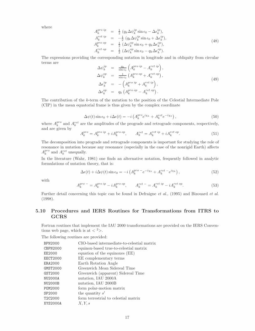
5.10 Procedures and IERS Routines for Transformations from ITRS toGCRS

Fortran routines that implement the IAU 2000 transformations are provided on the IERS Conven-tions web page, which is at < 2>.

The following routines are provided:BPN2000 CIO-based intermediate-to-celestial matrixCBPN2000 equinox-based true-to-celestial matrixEE2000 equation of the equinoxes (EE)EECT2000 EE complementary termsERA2000 Earth Rotation AngleGMST2000 Greenwich Mean Sidereal TimeGST2000 Greenwich (apparent) Sidereal TimeNU2000A nutation, IAU 2000ANU2000B nutation, IAU 2000BPOM2000 form polar-motion matrixSP2000 the quantity s′

T2C2000 form terrestrial to celestial matrixXYS2000A X,Y, s

17

The above routines are to a large extent self-contained, but in some cases use simple utility routinesfrom the IAU Standards Of Fundamental Astronomy software collection. This may be found at<3>. The SOFA collection includes its own implementations of the IAU 2000 models, togetherwith tools to facilitate their rigorous use. Two equivalent ways to implement the IAU Resolutionsin the transformation from ITRS to GCRS provided by expression (1) can be used, namely (a) thenew transformation based on the Celestial Intermediate Origin and the Earth Rotation Angle and(b) the classical transformation based on the equinox and Greenwich Sidereal Time. They arecalled respectively “CIO-based” and “equinox-based” transformations in the following.

For both transformations, the procedure is to form the various components of expression (1), ortheir classical counterparts, and then to combine these components into the complete terrestrial-to-celestial matrix.

Common to all cases is generating the polar-motion matrix, W (t) in expression (1), by callingPOM2000. This requires the polar coordinates xp, yp and the quantity s′; the latter can be estimatedusing SP2000.

The matrix for the combined effects of nutation, precession and frame bias is Q(t) in expression(1). For the CIO-based transformation, this is the intermediate-to-celestial matrix and can beobtained using the routine BPN2000, given the CIP position X,Y and the quantity s that definesthe position of the CIO. The IAU 2000A X,Y, s are available by calling the routine XYS2000A.In the case of the equinox-based transformation, the counterpart to matrix Q(t) is the true-to-celestial matrix. To obtain this matrix requires the nutation components Δψ and Δε; these can bepredicted using the IAU 2000A model by means of the routine NU2000A. Faster but lower-accuracypredictions are available from the NU2000B routine, which implements the IAU 2000B truncatedmodel. Once Δψ and Δε are known, the true-to-celestial matrix can be obtained by calling theroutine CBPN2000.

The intermediate component is the angle for Earth rotation that defines matrix R(t) in expression(1). For the CIO-based transformation, the angle in question is the Earth Rotation Angle, θ, whichcan be obtained by calling the routine ERA2000. The counterpart in the case of the equinox-basedtransformation is the Greenwich (apparent) Sidereal Time. This can be obtained by calling theroutine GST2000, given the nutation in longitude, Δψ, that was obtained earlier.

The three components are then assembled into the final terrestrial-to-celestial matrix by means ofthe routine T2C2000.

Three methods of applying the above scheme are set out below.

Method (1): CIO-based transformation consistent with IAU 2000A precession-nutation

This uses the new (X,Y, s, θ) transformation, which is consistent with IAU 2000A precession-nutation. Having called SP2000 to obtain the quantity s′, and knowing the polar motion xp, yp,the matrix W (t) can be obtained by calling POM2000. The Earth Rotation Angle provided byexpression (13) can be predicted with ERA2000, as a function of UT1. The X,Y, s series, basedon expressions (15) and (16) for X and Y , the coordinates of the CIP, and on Table 5.2c for thequantity s, that defines the position of the CIO, can be generated using the XYS2000A routine.(Note that this routine computes the full series for s rather than the summary model in Table 5.2c.)The matrix Q(t) that transforms from the intermediate system to the GCRS coordinates can thenbe generated by means of BPN2000. The finished terrestrial-to-celestial matrix is obtained bycalling the T2C2000 routine, specifying the polar-motion matrix, the Earth Rotation Angle andthe intermediate-to-celestial matrix.

Method (2A): the equinox-based transformation, using IAU 2000A precession-nutation

An alternative is the classical, equinox-based, transformation, using the IAU 2000A precession-nutation model and the new IAU-2000-compatible expression for GST.

3http://www.iau-sofa.rl.ac.uk

18

As for Method 1, the first step is to use SP2000 and POM2000 to obtain the matrix W (t), givenxp, yp. Next, compute the nutation components (lunisolar + planetary) by calling NU2000A. TheGreenwich (apparent) Sidereal Time is predicted by calling GST2000. This requires Δψ and TTas well as UT1. The matrix that transforms from the true equator and equinox of date to GCRScoordinates can then be generated by means of CBPN2000. Finally, the finished terrestrial-to-celestial matrix is obtained by calling the T2C2000 routine, specifying the polar-motion matrix,the Greenwich Sidereal Time and the intermediate-to-celestial matrix.

Method (2B): the classical transformation, using IAU 2000B precession-nutation

The third possibility is to carry out the classical transformation as for Method 2A, but based onthe truncated IAU 2000B precession-nutation model. Using IAU 2000B limits the accuracy toabout 1 mas, but the computations are significantly less onerous than when using the full IAU2000A model.

The same procedure as in Method (2A) is used, but substituting NU2000B for NU2000A. Dependingon the accuracy requirements, further efficiency optimizations are possible, including setting s′ tozero, omitting the equation of the equinoxes complementary terms and even neglecting the polarmotion.

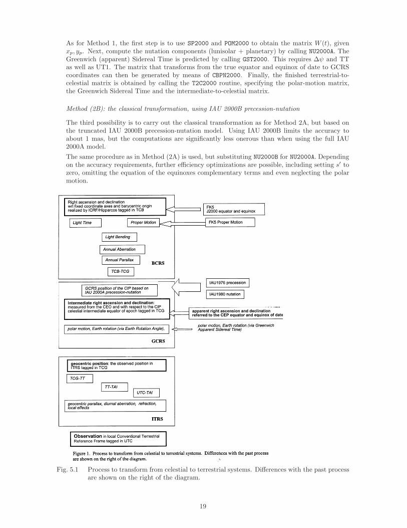
Fig. 5.1 Process to transform from celestial to terrestrial systems. Differences with the past processare shown on the right of the diagram.

19

5.11 Notes on the new Procedure to Transform from ICRS to ITRS

The transformation from the GCRS to ITRS, which is provided in detail in this chapter for use inthe IERS Conventions, is also part of the more general transformation for computing directions ofcelestial objects in intermediate systems.

The procedure to be followed in transforming from the celestial (ICRS) to the terrestrial (ITRS)systems has been clarified to be consistent with the improving observational accuracy. See Fig-ure 5.1 (McCarthy and Capitaine (in Capitaine et al., 2002)) for a diagram of the new and oldprocedures to be followed. As before, we make use of an intermediate reference system in trans-forming to a terrestrial system. In this case we call that system the Intermediate Celestial ReferenceSystem. (See also Seidelmann and Kovalevsky (2002).)

The Celestial Intermediate Pole (CIP) that is realized by the IAU2000A/B precession-nutationmodel defines its equator and the Conventional Intermediate Origin replaces the equinox.

The position in this reference system is called the intermediate right ascension and declination andis analogous to the previous designation of “apparent right ascension and declination.”

References

Cartwright, D. E. and Tayler, R. J., 1971, “New Computations of the Tide-Generating Potential,”Geophys. J. Roy. astr. Soc., 23, pp. 45–74.

Aoki, S., Guinot, B., Kaplan, G. H., Kinoshita, H., McCarthy, D. D., and Seidelmann, P. K., 1982,“The New Definition of Universal Time,” Astron. Astrophys., 105, pp. 359–361.

Aoki, S. and Kinoshita, H., 1983, “Note on the relation between the equinox and Guinot’s non-rotating origin,” Celest. Mech., 29, pp. 335–360.

Bizouard, Ch., Brzezinski, A., and Petrov, S., 1998, “Diurnal atmospheric forcing and temporalvariability of the nutation amplitudes,” J. Geod., 72, pp. 561–577.

Bizouard, Ch., Folgueira, M., and Souchay, J., 2000, “Comparison of the short period rigid Earthnutation series,” in Proc. IAU Colloquium 178, Publications of the Astron. Soc. Pac. Conf.Ser., Dick, S., McCarthy, D., and Luzum, B. (eds.), pp. 613–617.

Bizouard, Ch., Folgueira, M., and Souchay, J., 2001, “Short periodic nutations: comparison be-tween series and influence on polar motion,” in Proc. of the Journees 2000 Systemes deReference Spatio-Temporels, Capitaine, N. (ed.), Observatoire de Paris, pp. 260–265.

Bretagnon, P., 1982, “Theorie du mouvement de l’ensemble des planetes. solution VSOP82,”Astron. Astrophys., 114, pp. 278–288.

Bretagnon, P., Rocher, P., and Simon, J.-L., 1997. “Theory of the rotation of the rigid Earth,”Astron. Astrophys., 319, pp. 305–317.

Brzezinski, A., 2001, “Diurnal and subdiurnal terms of nutation: a simple theoretical model for anonrigid Earth,” in the Proc. of the Journees Systemes de Reference Spatio-temporels 2000,N. Capitaine (ed.), Observatoire de Paris, pp. 243–251.

Brzezinski, A., July 2002, Circular 2, IAU Commission 19 WG “Precession-nutation,” being pre-pared for publication.

Brzezinski, A., and Capitaine N., 2002, “Lunisolar perturbations in Earth rotation due to thetriaxial figure of the Earth: geophysical aspects,” in the Proc. of the Journees Systemes deReference Spatio-temporels 2001, N. Capitaine (ed.), Observatoire de Paris, pp. 51–58.

Buffett, B. A., Mathews, P. M., and Herring, T., 2002, “Modeling of nutation-precession: Effectsof electromagnetic coupling,” J. Geophys. Res., 107, B4, 10.1029/2001JB000056.

Capitaine, N., 1990, “The Celestial Pole Coordinates,” Celest. Mech. Dyn. Astr., 48, pp. 127–143.

Capitaine, N., 2000, “Definition of the Celestial Ephemeris Pole and the Celestial Ephemeris Ori-gin,” in Towards Models and Constants for Sub-Microarcsecond Astrometry, Johnston, K.J., McCarthy, D. D., Luzum, B. J., and Kaplan, G. H. (eds.), U.S. Naval Observatory, pp.153–163.

20

Capitaine, N., Guinot, B., and Souchay, J., 1986, “A Non-rotating Origin on the InstantaneousEquator: Definition, Properties and Use,” Celest. Mech., 39, pp. 283–307.

Capitaine, N. and Gontier A.-M., 1993, “Accurate procedure for deriving UT1 at a submilliarc-second accuracy from Greenwich Sidereal Time or from stellar angle,” Astron. Astrophys.,275, pp. 645–650.

Capitaine, N., Guinot, B., and McCarthy, D. D., 2000, “Definition of the Celestial Ephemeris originand of UT1 in the International Reference Frame,” Astron. Astrophys., 355, pp. 398–405.

Capitaine, N., Gambis, D., McCarthy, D. D., Petit, G., Ray, J., Richter, B., Rothacher, M., Stan-dish, M., and Vondrak, J., (eds.), 2002, IERS Technical Note, 29 Proceedings of the IERSWorkshop on the Implementation of the New IAU Resolutions, 2002,http://www.iers.org/iers/publications/tn/tn29/, Verlag des Bundesamts fur Kartogra-phie und Geodasie, Frankfurt am Main.

Capitaine, N., Chapront, J., Lambert, S., and Wallace, P., 2003a, “Expressions for the CelestialIntermediate Pole and Celestial Ephemeris Origin consistent with the IAU 2000A precession-nutation model,” Astron. Astrophys., 400, pp. 1145–1154.

Capitaine, N., Wallace, P. T., and McCarthy, D. D., 2003b, “Expressions to Implement the IAU2000 Definition of UT1,” Astron. Astrophys., 406, pp. 1135-1149.

Capitaine, N., Wallace, P. T., and Chapront, J., and 2003c, “Expressions for IAU 2000 precessionquantities,” accepted to Astron. Astrophys..

Chapront-Touze, M. and Chapront, J., 1983, “The lunar ephemeris ELP 2000,” Astron. Astro-phys., 124, pp. 50–62.

Chapront, J., Chapront-Touze, M. and Francou, G., 2002, “A new determination of lunar orbitalparameters, precession constant and tidal acceleration from LLR measurements,” Astron.Astrophys., 387, pp. 700–709.

Defraigne, P., Dehant, V., and Paquet, P., 1995, “Link between the retrograde-prograde nutationsand nutations in obliquity and longitude,” Celest. Mech. Dyn. Astr., 62, pp. 363–376.

Dehant, V., Arias, F., Bizouard, Ch., Bretagnon, P., Brzezinski, A., Buffett, B., Capitaine, N.,Defraigne, P., de Viron, O., Feissel, M., Fliegel, H., Forte, A., Gambis, D., Getino, J., Gross.,R., Herring, T., Kinoshita, H., Klioner, S., Mathews, P. M., McCarthy, D., Moisson, X.,Petrov, S., Ponte, R. M., Roosbeek, F., Salstein, D., Schuh, H., Seidelmann, K., Soffel, M.,Souchay, J., Vondrak, J., Wahr, J. M., Weber, R., Williams, J., Yatskiv, Y., Zharov, V., andZhu, S. Y., 1999, “Considerations concerning the non-rigid Earth nutation theory,” Celest.Mech. Dyn. Astr., 72, pp. 245–310.

Escapa, A., Getino, J., and Ferrandiz, J. M., 2002a, “Indirect effect of the triaxiality in theHamiltonian theory for the rigid Earth nutations,” Astron. Astrophys., 389, pp. 1047–1054.

Escapa, A., Getino, J., and Ferrandiz, J. M., 2002b, “Influence of the triaxiality of the non-rigidEarth on the J2 forced nutations,” in the Proc. of the Journees Systemes de Reference Spatio-temporels 2001, N. Capitaine (ed.), Observatoire de Paris, pp. 275–281.

Folgueira, M., Souchay, J., and Kinoshita, S., 1998a, “Effects on the nutation of the non-zonalharmonics of third degree,” Celest. Mech. Dyn. Astr., 69, pp. 373–402.

Folgueira, M., Souchay, J., and Kinoshita, S., 1998b, “Effects on the nutation of C4m and S4mharmonics,” Celest. Mech. Dyn. Astr., 70, pp. 147–157.

Folgueira, M., Bizouard, C., and Souchay, J., 2001, “Diurnal and subdiurnal luni-solar nutations:comparisons and effects,” Celest. Mech. Dyn. Astr., 81, pp. 191–217.

Fukushima, T., 1991, “Geodesic Nutation,” Astron. Astrophys., 244, pp. L11–L12.

Getino, J., Ferrandiz, J. M. and Escapa, A., 2001, “Hamiltonian theory for the non-rigid Earth:semi-diurnal terms,” Astron. Astrophys., 370, pp. 330–341.

Guinot, B., 1979, “Basic Problems in the Kinematics of the Rotation of the Earth,” in Time andthe Earth’s Rotation, McCarthy, D. D. and Pilkington, J. D. (eds.), D. Reidel PublishingCompany, pp. 7–18.

21

Herring, T., Mathews, P. M., and Buffett, B. A., 2002, “Modeling of nutation-precession: Verylong baseline interferometry results,” J. Geophys. Res., 107, B4, 10.1029/2001JB000165.

Kinoshita, H. and Souchay, J., 1990, “The theory of the nutations for the rigid Earth at the secondorder,” Celest. Mech. and Dyn. Astron., 48, pp. 187–265.

Lambert, S. and Bizouard, C., 2002, “Positioning the Terrestrial Ephemeris Origin in the Inter-national Terrestrial Frame,” Astron. Astrophys., 394, pp. 317–321.

Lieske, J. H., Lederle, T., Fricke, W., and Morando, B., 1977, “Expressions for the PrecessionQuantities Based upon the IAU (1976) System of Astronomical Constants,” Astron. Astro-phys., 58, pp. 1–16.

Ma, C., Arias, E. F., Eubanks, T. M., Fey, A., Gontier, A.-M., Jacobs, C. S., Sovers, O. J.,Archinal, B. A., and Charlot, P., 1998, “The International Celestial Reference Frame asrealized By Very Long Baseline Interferometry,” Astron. Astrophys., 116, pp. 516–546.

Mathews, P. M., Herring, T. A., and Buffett B. A., 2002, “Modeling of nutation-precession: Newnutation series for nonrigid Earth, and insights into the Earth’s Interior,” J. Geophys. Res.,107, B4, 10.1029/2001JB000390.

Mathews, P. M. and Bretagnon, P., 2002, “High frequency nutation,” in the Proc. of the JourneesSystemes de Reference Spatio-temporels 2001, N. Capitaine (ed.), Observatoire de Paris, pp.28–33.

McCarthy, D. D. (ed.), 1996, IERS Conventions, IERS Technical Note, 21, Observatoire de Paris,Paris.

McCarthy, D. D. and Luzum, B. J., 2003, “An Abridged Model of the Precession-Nutation of theCelestial Pole,” Celest. Mech. Dyn. Astr., 85, pp. 37–49.

Roosbeek, F., 1999,“Diurnal and subdiurnal terms in RDAN97 series,” Celest. Mech. Dyn. Astr.,74, pp. 243–252.

Seidelmann, P. K., 1982, “1980 IAU Nutation: The Final Report of the IAU Working Group onNutation,” Celest. Mech., 27, pp. 79–106.

Seidelmann, P. K. and Kovalevksy, J., 2002, “Application of the new concepts and definitions(ICRS, CIP and CEO) in fundamental astronomy,” Astron. Astrophys., 392, pp. 341–351.

Simon, J.-L., Bretagnon, P., Chapront, J., Chapront-Touze, M., Francou, G., and Laskar, J.,1994, “Numerical Expressions for Precession Formulae and Mean Elements for the Moon andPlanets,” Astron. Astrophys., 282, pp. 663–683.

Souchay, J. and Kinoshita, H., 1997, “Corrections and new developments in rigid-Earth nuta-tion theory. II. Influence of second-order geopotential and direct planetary effect,” Astron.Astrophys., 318, pp. 639–652.

Souchay, J., Loysel, B., Kinoshita, H., and Folgueira, M., 1999, “Corrections and new developmentsin rigid Earth nutation theory: III. Final tables REN-2000 including crossed-nutation andspin-orbit coupling effects,” Astron. Astrophys. Supp. Ser., 135, pp. 111–131.

Standish, E. M., 1981, “Two differing definitions of the dynamical equinox and the mean obliquity,”Astron. Astrophys., 101, p. L17.

Wahr, J. M., 1981, “The forced nutation of an elliptical, rotating, elastic and oceanless Earth,”Geophys. J. R. astr. Soc., 64, pp. 705–727.

Williams, J. G., Newhall, X. X., and Dickey, J. O., 1991, “Luni-solar precession — Determinationfrom lunar laser ranges,” Astron. J., 241, pp. L9–L12.

Williams, J. G., 1994, “Contributions to the Earth’s obliquity rate, precession, and nutation,”Astron. J., 108, pp. 711–724.

22