5 natural abundance of the stable isotopes … i/cht_i_07.pdf · 7 natural abundance of the stable...

7 NATURAL ABUNDANCE OF THE STABLE ISOTOPES OF C, O AND H

This chapter is concerned with the natural concentrations of the stable isotopes of hydrogen, carbon and oxygen, with particular attention paid to those compounds relevant in the hydrological cycle. For each isotope separately, we discuss the natural fractionation effects, internationally agreed definitions, standards, and reference materials, and variations in the natural abundances.

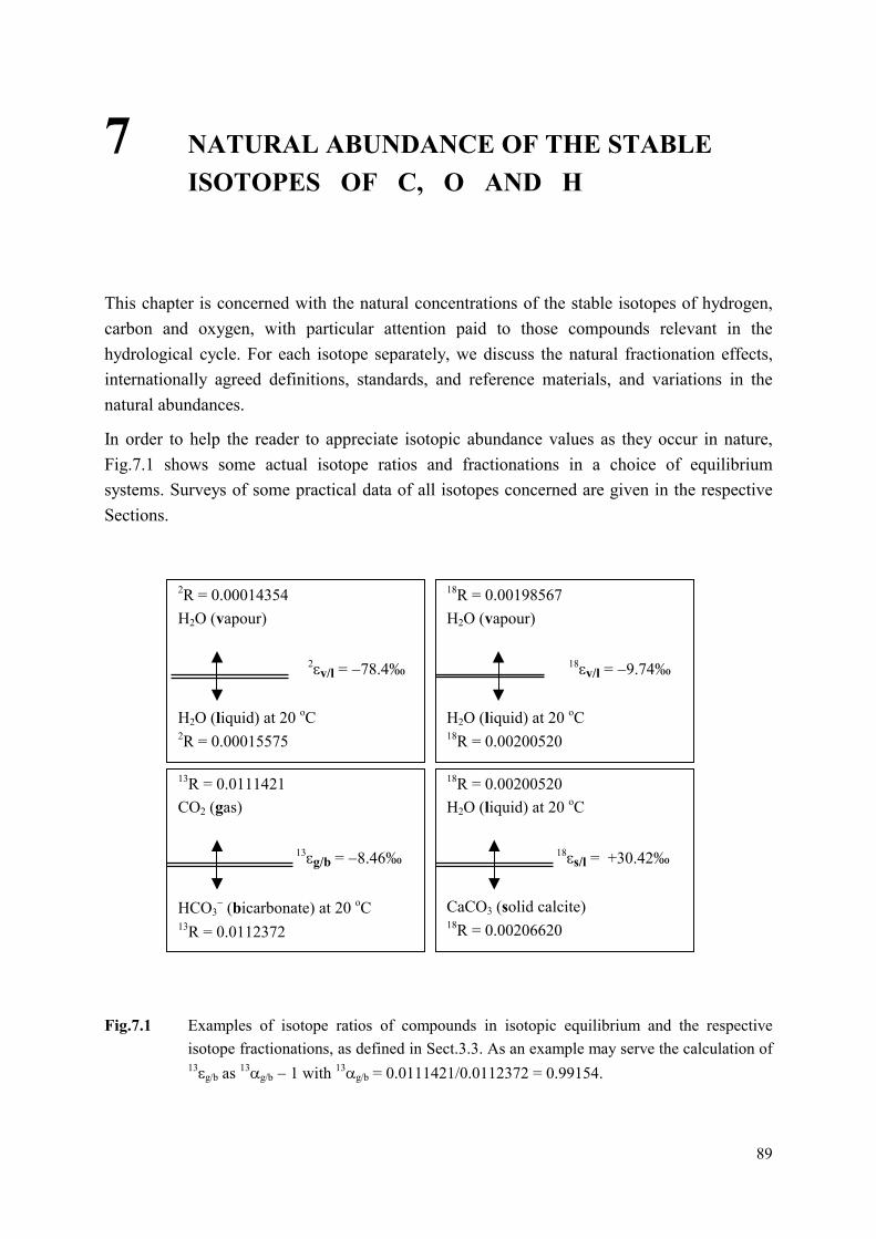
In order to help the reader to appreciate isotopic abundance values as they occur in nature, Fig.7.1 shows some actual isotope ratios and fractionations in a choice of equilibrium systems. Surveys of some practical data of all isotopes concerned are given in the respective Sections.

18R = 0.00200520 H2O (liquid) at 20 oC

18�s/l = +30.42‰

CaCO3 (solid calcite) 18R = 0.00206620

13R = 0.0111421 CO2 (gas)

13�g/b = �8.46‰

HCO3

� (bicarbonate) at 20 oC 13R = 0.0112372

18R = 0.00198567 H2O (vapour)

18�v/l = �9.74‰

H2O (liquid) at 20 oC 18R = 0.00200520

2R = 0.00014354 H2O (vapour)

2�v/l = �78.4‰ H2O (liquid) at 20 oC 2R = 0.00015575

Fig.7.1 Examples of isotope ratios of compounds in isotopic equilibrium and the respective isotope fractionations, as defined in Sect.3.3. As an example may serve the calculation of 13�g/b as 13

�g/b � 1 with 13�g/b = 0.0111421/0.0112372 = 0.99154.

89

Chapter 7

7.1 STABLE CARBON ISOTOPES

Table 7.1 The stable and radioactive isotopes of carbon: practical data for the natural abundance, properties, analytical techniques and standards. Further details are given in Sect.7.1 and 8.1, and in Chapters 10 and 11.

MS = mass spectrometry, PGC = proportional gas counting, LSS = liquid scintillation spectrometry, AMS = accelerator mass spectrometry

12C 13C 14C

stability stable stable radioactive

natural abundance 0.989 0.011 < 10�12

natural specific activity < 0.25 Bq/gC

decay mode / daughter �� / 14N

half-life (T1/2) 5730 a

decay constant (�) 1.21�10�4/a = 1/8267 a�1

max. � energy 156 keV

abundance range in hydrological cycle

30‰ 0 to 10�12

reported as 13� or �13C 14A, 14a, 14

�, or 14�

in ‰ dpm/gC, Bq/gC, %, or ‰

instrument MS PGC, LSS, AMS

analytical medium CO2 CO2, C2H2, CH4, C6H6, graphite

usual standard deviation 0.03‰ 1‰ to 1% at natural level

international standard VPDB Oxalic acid: Ox1, Ox2

with absolute value 0.0112372 13.56 dpm/gC

7.1.1 THE NATURAL ABUNDANCE

The chemical element carbon has two stable isotopes, 12C and 13C. Their abundance is about 98.9% and 1.1%, so that the 13C/12C ratio is about 0.011 (Nier, 1950). As a result of several fractionation processes, kinetic as well as equilibrium, the isotope ratio shows a natural variation of almost 100‰.

90

Stable Isotopes of Hydrogen, Carbon and Oxygen

Fig.7.2 General view of 13C/12C variations in natural compounds. The ranges are indicative for the materials shown.

atmospheric CO2 marine HCO3

� marine carbonate marine plants marine plankton land plants C4 type land plants C3 type groundwater HCO3

� fresh-water carbonate wood peat coal oil natural gas bacterial CH4 animal bone diamond

�80 �60 �40 �20 0 +2013�VPDB (‰)

Fig.7.2 presents a broad survey of natural abundances of various compounds, at the low-13C end bacterial methane (marsh-gas), at the high end the bicarbonate fraction of groundwater under special conditions. In the carbonic acid system variations up to 30‰ are normally observed. Wider variations occur in systems in which carbon oxidation or reduction reactions take place, such as the CO2 (carbonate) � CH4 (methane) or the CO2 � (CH2O)x (carbohydrate) systems.

7.1.2 CARBON ISOTOPE FRACTIONATIONS

It will later be shown that the presence of dissolved inorganic carbon (DIC) in sea-, ground-, and surface water presents the possibility of studying gas-water exchange processes and of measuring water transport rates in oceans and in the ground. In connection with studying these phenomena, the stable and radioactive isotopes of carbon and their interactions pay an important contribution, often together with the water chemistry.

91

Chapter 7

CO32�

CaCO3

CO2 g

CO2 aq

temperature t (�C)

fractionation 13� (‰)

40 302010 0

4

0

-4

-8

-12

g/b

a/b

c/b

s/b

HCO3�

Fig.7.3 Temperature-dependent equilibrium isotope fractionation for carbon isotopes of gaseous CO2 (g), dissolved CO2 (a), dissolved carbonate ions (c), and solid carbonate (s) with respect to dissolved HCO3

� (b). The actual data and equations are given in Table 7.2.

In nature equilibrium carbon isotope effects occur specifically between the phases CO2 � H2O � H2CO3 � CaCO3. Values for the fractionations involved only depend on temperature and are obtained from laboratory experiments. A survey is presented in Fig.7.3 and Table 7.2.

The kinetic fractionation of specific interest is that during carbon dioxide assimilation, i.e. the CO2 uptake by plants. The relatively large fractionation (up to about �18‰) is comparable to the effect observed during absorption of CO2 by an alkaline solution. A quantitative estimate shows that the isotope effect as a result of diffusion of CO2 through air can not explain the fractionation (Sect.3.5). The resulting value of 13

� is 0.9956, so that only �4.4‰ of the total assimilation fractionation in favour of 12C can be explained by the diffusion. The remaining �13.6‰, therefore, has to be found in the surface of the liquid phase and in the subsequent biochemical process.

92


Table 7.2 Carbon isotope fractionation in the equilibrium system CO2�HCO3�CO3�CaCO3; 13�y/x represents the fractionation of compound y relative to compound x. Values for

intermediate temperatures may be calculated by linear interpolation (see also Fig.7.3). T = t (�C) + 273.15 K

g = gaseous CO2 , a = dissolved CO2 , b = dissolved HCO3� , c = dissolved CO3

2� ions, s = solid calcite.

t (�C)

13�g/b 1) (‰)

13�a/g 2) (‰)

13�a/b 3) (‰)

13�c/b 4) (‰)

13�s/b 5) (‰)

13�s/g 6) (‰)

0 �10.83 � 1.18 �12.00 � 0.65 � 0.39 +10.55 5 �10.20 � 1.16 �11.35 � 0.60 � 0.11 +10.19

10 � 9.60 � 1.13 �10 72 � 0.54 + 0.15 + 9.85 15 � 9.02 � 1.11 �10.12 � 0.49 + 0.41 + 9.52 20 � 8.46 � 1.09 � 9.54 � 0.44 + 0.66 + 9.20 25 � 7.92 � 1.06 � 8.97 � 0.39 + 0.91 + 8.86 30 � 7.39 � 1.04 � 8.42 � 0.34 + 1.14 + 8.60 35 � 6.88 � 1.02 � 7.90 � 0.29 + 1.37 + 8.31 40 � 6.39 � 1.00 � 7.39 � 0.25 + 1.59 + 8.03

1) Mook et al., 1974 :13

�g/b = � 9483/T + 23.89‰ (7.1) 2) Vogel et al., 1970 :13

�a/g = � 373/T + 0.19‰ (7.2) 3) From 1) and 2) :13

�a/b = � 9866/T + 24.12‰ (7.3) 4) Thode et al., 1965 and 1) :13

�c/b = � 867/T + 2.52‰ (7.4) 5) Our evaluation of the original data from Rubinson & Clayton, 1969

and Emrich et al., 1970 :13�s/b = � 4232/T + 15.10‰ (7.5)

6) From 1) and 5) :13�s/g = + 5380/T � 9.15‰ (7.6)

Another kinetic process occurring in the soil is the bacterial decomposition of organic matter to form methane (CH4). Here the largest fractionation amounts to about �55‰. In this process CO2 is simultaneously produced with a fractionation of +25‰, resulting in a 13

� value of about 0‰. A special problem is the kinetic fractionation during uptake and release of CO2 by seawater. This fractionation is included in calculations on global 13C modelling.

First we have to emphasise that the difference in isotopic composition between, for instance, gaseous CO2 and the dissolved inorganic carbon content of water can not be addressed by isotope fractionation between CO2 and DIC.

93

Chapter 7

13� (‰) rel. to air�CO2

pH=8.2 20 �C kineticequilibrium +2

�2

�4

�6

+6

�8

�4

�2

+8

+4

+2

0

0

�10

�12

atmospheric CO2

HCO3�

CO32�

oceanic DIC

CO2 CO2(aq)

13�VPDB (‰)

13�c/g

13�b/g 13

��/g13�(sea�air)

13�(air�sea)

CO2 taken up released by the sea

13�a-g

+10

Fig.7.4 Fractionation for the isotopic equilibrium between CO2(gas)�dissolved CO2(aq)�dissolved bicarbonate (HCO3

�)�dissolved carbonate (CO32�) (Mook, 1986). The

right-hand scale indicates approximate natural 13� values with respect to VPDB. The

right-hand part shows kinetic fractionations during uptake and release of atmospheric oceanic CO2, respectively. DIC is the total dissolved inorganic carbon content (CT).

Isotope fractionation is the phenomenon that, due to an isotope exchange process, a difference between the isotopic composition of two compounds occurs, while seawater carbon consists of 3 fractions, i.e. dissolved CO2 (H2CO3 is hardly present), dissolved HCO3

�, and dissolved CO3

2�. All these fractions are fractionated isotopically with respect to each other. The 13R value of DIC is:

]CO[+]HCO[+]aqCO[

R]CO[+R]HCO[+R]aqCO[=R 2

332

3CO132

33HCO13

3aq2CO13

2DIC

13

or in terms of the respective fractionations:

b13

T

b/c13

b/a13

DIC13 R

Ccba

R��

� (7.7)

94


or in terms of � values:

T

b/c13

b/a13

b13

T

b/c13

b/a13

DIC13

Cca

Ccba ��

��

�� (7.8)

where the brackets indicate the respective concentrations, which are also denoted by a (acid), b (bicarbonate), and c (carbonate ions), so that a + b + c = CT. The � values are given in Table 7.2. The chemical fractions are quantitatively treated in Chapter 9.

Originally 13�k values for the uptake of CO2 by seawater of about �15‰ were assumed, based

on experimental results of CO2 absorption by an alkaline solution (Baertschi, 1952). However, Siegenthaler & Münnich (1981) have reasoned that this effect does not apply to the dissolving action of seawater. Calculations by these authors as well as by Inoue & Sugimura (1985) and Wanninkhof (1985) have shown the kinetic fractionation during CO2 uptake to be

13�k (air � sea) = 13

�k (atm.CO2 to CO2 taken up) = �2.0 ± 0.2‰

This value was confirmed by experiments of the last author (�2.4 ± 0.8‰).(We have to remind the reader that these 13

�k values as well as those below are for kinetic fractionations and do not refer to Table 7.2).

The kinetic fractionation during CO2 release by the ocean reported by Siegenthaler & Münnich (1981) needs a correction (Mook, 1986). By application of the most recent equilibrium fractionations of Table 7.2 the equilibrium fractionation (13

�a/DIC) for dissolved CO2 with respect to total dissolved carbon at 20 oC is 0.99055. This fractionation factor is also determined by the chemical composition of seawater, which adds to the overall temperature dependence.

At 20 oC the respective relative concentrations in seawater at pH = 8.20 are: CO2(aq)/CT = 0.006, HCO3

�/CT = 0.893 and CO32�/CT = 0.102 where CT is the total inorganic carbon

concentration. By incorporation of the CO2 + OH� reaction (0.9995), the resulting 13� value is

�10.1 to �10.6‰, depending on whether the hydration of CO2 to H2O is to be included.

According to Inoue & Sugimura (1985) the value is about -10‰, so that we can conclude to a fractionation of released CO2 with respect to DIC of:

13�k (sea � air) = 13

�k (DIC rel. to CO2 released) = �10.3 ± 0.3‰

Figure 7.4 represents a review of equilibrium and kinetic fractionations relative to gaseous CO2 (left-hand scale) and the actual 13

� values based on 13� (atm.CO2) = �7.0‰ (right-hand

scale). It is obvious that the isotopic compositions of CO2 released and taken up by the ocean are equal, as is required by the condition of stationary state of isotopic equilibrium between ocean and atmosphere.

95

Chapter 7

7.1.3 REPORTING 13C VARIATIONS AND THE 13C STANDARD

As described in Sect.4.1, isotopic compositions expressed as 13� values are related to those of

specific reference materials. By international agreement PDB was used as the primary carbon reference (standard) material. PDB (Pee Dee Belemnite) was the carbonate from a certain (marine) belemnite found in the Cretaceous Pee Dee formation of North America. This material was the original standard sample used in the early days in Chicago and at CalTech, but has long been exhausted. The US National Bureau of Standards therefore distributed another (marine) limestone of which 13

� had been accurately established in relation to PDB. This first standard available to the community, Solenhofen limestone NBS20, was analysed by Craig (1957) and consecutively defined as: 13

�NBS20 / PDB = �1.06‰

In this way the PDB scale was indirectly established. Meanwhile NBS20 is considered to be no longer reliable, probably because of improper storage, and has been replaced by another limestone, NBS19, of which the 13

� value has been compared by a number of laboratories with the previous standard.

Based on this comparison an IAEA panel in 1983 (Gonfiantini, 1984) adopted this new standard to define the new VPDB (Vienna PDB) scale as: 13

�NBS19 / VPDB = +1.95‰ (7.9)

The absolute 13C/12C ratio of PDB was originally reported as 0.0112372 (Craig, 1957), whereas a slightly different value of 0.011183 (� 0.1‰) was reported by Zhang and Li (1987). The distinction between PDB and VPDB has been made for formal reasons, but the difference is negligibly small (< 0.01‰).

Henceforth all 13� values are reported relative to VPDB, unless stated otherwise.

More details on measurement and calculation procedures are given in Chapter 11. A survey of other reference samples is given in Table 11.2.

7.1.4 SURVEY OF NATURAL 13C VARIATIONS

In the other volumes certain aspects of natural 13� variations will be discussed in more detail.

Here we will restrict ourselves to a general survey, particularly with regard to the hydrological cycle (Fig. 7.5).

7.1.4.1 ATMOSPHERIC CO2

The least depleted atmospheric CO2 had originally 13� values near �7‰. Since the 19th

century this value has undergone relatively large changes. In general, high values are observed in

96


5 �C

exchange with soil CO2

groundwater HCO3�

atmospheric CO2

exchange with atmosphere

13�VPDB (‰)

25�C

+ 5

0

� 5

�30

�20

�10

C3 plants

soil CO2

C4 plants

marine bicarbonate calcite

freshwater bicarbonate calcite

�15

�25

�40

�35

coal oil

natural gas (CH4)

Fig.7.5 Schematic survey of 13

� variations in nature, especially of compounds relevant in the hydrological cycle.

97

Chapter 7

oceanic air far removed from continental influences and occurs in combination with minimal CO2 concentrations. More negative 13

� values are found in continental air and are due to an admixture of CO2 of biospheric and anthropogenic origin (13

� � �25‰), in part from the decay of plant material, in part from the combustion of fossil fuels (Keeling, 1958; Mook et al., 1983).

7.1.4.2 SEAWATER AND MARINE CARBONATE

Atmospheric CO2 appears to be nearly in isotopic equilibrium with the oceanic dissolved bicarbonate. The 13

�(HCO3�) values in the ocean are about +1 to +1.5‰, in agreement with

the equilibrium fractionation �g/b at temperatures between 15 and 20 �C (Table 7.2). According to the fractionation �s/b we should expect calcite slowly precipitating in equilibrium with oceanic bicarbonate to have 13

� values of +2.0 to +2.5‰. This is indeed the normal range found for recent marine carbonates. Mook and Vogel (1968) observed this isotopic equilibrium between marine to brackish-water shells and dissolved bicarbonate in the water.

7.1.4.3 VEGETATION AND SOIL CO2

Plant carbon has a lower 13C content than the atmospheric CO2 from which it was formed. The fractionation which occurs during CO2 uptake and photosynthesis depends on the type of plant and the climatic and ecological conditions. The dominant modes of photosynthesis give rise to strongly differing degrees of fractionation (Lerman, 1972; Throughton, 1972). The Hatch-Slack photosynthetic pathway (C4) results in 13

� figures of �10 to �15‰ and is primarily represented by certain grains and desert grasses (sugar reed, corn). In temperate climates most plants employ the Calvin mechanism (C3), producing 13

� values in the range of �26 � 3‰. A third type of metabolism, the Crassulacean Acid Metabolism (CAM) produces a large spread of 13

� values around �17‰ (Deines, 1980).

The CO2 content of the soil atmosphere can be orders of magnitude larger than that of the free atmosphere. The additional CO2 is formed in the soil by decay of plant remains and by root respiration and consequently has 13

� values centring around �25‰ in temperate climates where Calvin plants dominate.

7.1.4.4 FOSSIL FUEL

As complicated biogeochemical processes are involved in the degradation of terrestrial and marine plant material ultimately into coal, oil, and natural gas, the range of 13

� values of these fossil fuels is larger, extending to more negative values, especially of biogenic methane (Fig.7.5). The global average of CO2 from the combustion of these fuels is estimated to be about �27‰.

98


7.1.4.5 GLOBAL CARBON CYCLE

Biospheric carbon has a direct influence on 13� of atmospheric CO2. The large uptake of CO2

by the global biosphere during summer and the equal release of CO2 during winter causes a seasonal variation in the atmospheric CO2 concentration as well as in 13

�. The simple mixing of CO2 from these two components, atmospheric CO2 (atm) and biospheric CO2 (bio) is represented by the equation (cf. Eqs.4.13 and 4.15):

(13�atm + 13

�)(Catm + Cbio) = 13�atmCatm + 13

�bioCbio (7.10)

where C stands for the CO2 concentration, C for the biospheric addition, and 13� for the

variation in the � value.

330

335

340

345

350

355

360

1978 1980 1982 1984 1986 1988 1990 1992 1994 1996

-7.9

-7.8

-7.7

-7.6

-7.5

-7.41978 1980 1982 1984 1986 1988 1990 1992 1994 1996

Mauna Loa Hawaii

South

South Pole

Mauna Loa

13�VPDB (‰)

CO2 concentration (ppm)

Fig.7.6 Trends of the concentration and 13� of atmospheric CO2 of air samples collected by

C.D.Keeling on top of the Mauna Loa volcano at the Island of Hawaii and at the South Pole. The seasonal variations have been removed from the original data (Roeloffzen et al., 1991). The dates refer to 1 January of each year.

99

Chapter 7

Numerically this comes to a periodic (seasonal) variation of

2000

bioatm

atm13

bio13

bio

13COofppmper05.0

35385.725

CCC��

��

��

��

�

�� (7.11)

Superimposed on this phenomenon is the gradual increase in the concentration and the accompanying decrease in 13

� by the emission of fossil-fuel CO2. The trends are shown in Fig.7.6 and can be approximated by:

13� / CO2 = �0.015 ‰ / ppm or 13

� = �0.025‰ / year (7.12)

at a CO2 concentration of 353 ppm and 13� = �7.85‰ over the Northern Hemisphere, valid

for 01/01/1990.

The smaller ‰/ppm value of Eq.7.12 compared to Eq.7.11 shows that the long-term trend is not due to simple addition and mixing of additional CO2 in the atmosphere. The large oceanic DIC reservoir is levelling out the purely atmospheric mixing effect through isotope exchange.

7.1.4.6 GROUNDWATER AND RIVERWATER

Soil CO2 is important in establishing the dissolved inorganic carbon content of groundwater. After dissolution of this CO2 the infiltrating rain water is able to dissolve the soil limestone:

CO2 + H2O + CaCO3 Ca2+ + 2HCO3� (7.13)

(Fig.7.7). Because limestone generally is of marine origin (13� � +1‰), this process results in

13� of the dissolved bicarbonate of about �11 to �12‰ (in temperate climates).

In the soil the HCO3� first formed exchanges with the often present excess of gaseous CO2,

ultimately resulting in 13�(HCO3

�) = 13�(soil CO2) + 13

�b/g � �25‰ + 9‰ = �16‰ (Fig.7.5). Consequently, 13

�(HCO3�) values significantly outside the range of �11 to �12‰ are

observed in soil water as well as in fresh surface water such as rivers and lakes. In surface waters such as lakes 13C enrichment of dissolved inorganic carbon can be caused by isotope exchange with atmospheric CO2 (13

� � �7.5‰), ultimately resulting in values of 13� + 13

�b/g = �7.5‰ + 9‰ = +1.5‰, identical to oceanic values. Consequently, freshwater carbonate minerals may have "marine" 13

� values. In these cases the marine character of the carbonate is to be determined by 18

� (Sect.7.3).

In addition to HCO3�, natural waters contain variable concentrations of CO2 with the effect

that the 13� value of DIC is lower than that of the bicarbonate fraction alone: in groundwater

(Vogel and Ehhalt, 1963), and in stream and river waters derived from groundwater (Fig.7.8) the 13

�(DIC) values are generally in the range of �12 to �15‰.

100


marine CaCO3+ 1‰

plants / humus� 25‰

humus CO2

� 25‰

soil CaCO3+ 1 ± 1‰

dissolved CO2

� 25 ± 1‰

soil H2O

atmosph.CO2

� 7.5‰

groundwaterHCO3

�

� 12 ± 1‰

exchange precipitation

erosion / sedimentation

groundwaterDIC�11 to �16‰

oceanic HCO3�

+ 1‰

Fig. 7.7 Schematic representation of the formation of dissolved inorganic carbon in groundwater from soil carbonate and soil CO2. This is the main process responsible for the carbonate content of groundwater and the consecutive components of the water cycle. Generally, dissolved bicarbonate is by far the largest component. The ‰ values referring to the respective 13

� have been kept simple for the sake of clarity. DIC is the dissolved inorganic carbon content of the water, i.e. HCO3

�, CO2(aq) and CO32�.

7.2 STABLE OXYGEN ISOTOPES


The chemical element oxygen has three stable isotopes, 16O, 17O and 18O, with abundances of 99.76, 0.035 and 0.2%, respectively (Nier, 1950). Observation of 17O concentrations provides little information on the hydrological cycle in the strict sense above that which can be gained from the more abundant and, consequently, more accurately measurable 18O variations (Sect.3.7). We shall, therefore, focus our attention here on the 18O/16O ratio (� 0.0020).

Values of 18� show natural variations within a range of almost 100‰ (Fig.7.9). 18O is often

enriched in (saline) lakes subjected to a high degree of evaporation, while high-altitude and cold-climate precipitation, especially in the Antarctic, is low in 18O. Generally in the hydrological cycle in temperate climates we are confronted with a range of 18

� not exceeding 30‰.

101

Chapter 7

18�(H2O) (‰)

Meuse

Rhine

B

36 24 12 0

-6

-7

-8

-9

-10

-11

Rhine

Meuse

13�(HCO3

�) (‰)

A

0 12 24 36 12 2 4 6 8 10 12 2 4 6 8 10 12 2 4 6 8 10 12 1967 1968 1969

-6

-8

-10

-12

-14

Fig.7.8 A three-year observation of the isotopic composition of water from the N.W.European rivers Rhine and Meuse (Mook, 1970):

A. 13� values of the dissolved bicarbonate fraction, showing normal values during winter

and relatively high values in summer, probably because of isotopic exchange of the surface water bicarbonate with atmospheric CO2.

B. 18� values, where the river Meuse is showing the average value and the seasonal

variations of 18� in the precipitation: high values in summer, low during winter; during

early spring and summer the Rhine receives meltwater from the Swiss Alps with relatively low 18

� because of the high-altitude precipitation .

102


Table 7.3 The stable isotopes of oxygen: practical data for the natural abundance, properties, analytical techniques and standards. Further details are given in Sect.7.2, and in Chapters 10 and 11.

MS=mass spectrometry

16O 17O 18O

stability stable stable stable

natural abundance 0.9976 0.00038 0.00205

abundance range in hydrological cycle

15‰ 30‰

reported as 17� or �17O 18

� or �18O

in ‰ ‰

instrument MS MS

analytical medium O2 CO2 or O2

usual standard deviation 0.05‰

international standard . VSMOW for water

VPDB for carbonate etc

with absolute value VSMOW: 0.0020052

VPDB: 0.0020672

7.2.2 OXYGEN ISOTOPE FRACTIONATIONS

The isotope effects to be discussed are within the system H2O (vapour) � H2O (liquid) � CaCO3. The equilibrium fractionation values have been determined by laboratory experiments. Fig.7.1 shows some actual isotope ratios. Fig.7.10 and Table 7.4 present a survey of the temperature dependent equilibrium isotope effects.

Equilibrium fractionations determined in the laboratory are also found in nature. The most striking observation is that the carbonate shells of many molluscs appear to have been formed in isotopic equilibrium with seawater. The palaeotemperature scale as presented by Eq.7.18 was presented by Epstein et al. (1953) (cf. Friedman & O'Neil, 1977). This relation is deduced from 18O measurements on carbonate laid down by marine shell animals at known temperatures and water isotopic compositions. These data lost the original interpretation of the temperature dependence of the �s/l by the later realisation that the major oceanic palaeotemperature effect is the change in 18

� of seawater –and, consequently of carbonate formed in this water- by the formation viz. melting of enormous ice caps on the poles during or after ice ages.

103

Chapter 7

18�VSMOW (‰)

�20 0 +20 +40 +60

for water 18�VSMOW (‰)

for carbonate 18�VPDB (‰)

ocean water arctic sea ice marine moisture (sub)tropical precipitation Dead Sea/Lake Chad temperate zone precipitation Alpine glaciers Greenland glaciers Antarctic ice Quatern. marine carbonates fresh-water carbonates ocean water marine carbonates igneous rocks marine atmospheric CO2 atmospheric oxygen organic matter

�60 �40 �20 0 +20

Fig.7.9 General view of 18O/16O variations in natural compounds. The ranges are indicative for the majority of materials shown. The relation between the VPDB and VSMOW scales is given in Sect.7.2.3 and Fig.7.11.

Kinetic effects are observed during the evaporation of ocean water, as oceanic vapour is isotopically lighter than would result from equilibrium fractionation alone. The natural isotope effect for oxygen (� -12‰) is smaller than could be brought about by fractionation by diffusion. Laboratory measurements resulted in 18

�d = -27.3 ± 0.7‰ (Merlivat, 1978) and 18�d

= -27.2 ± 0.5‰ (unpubl.). These experimental values are again smaller than results from Eq.(3.35) (-31.3‰), which may be explained by the water molecules forming clusters of

104


-20

-10

0

10

20

30

40

50

0 10 20 30 40

CaCO3 solid

CO2 gas

H2O liquid

H2O vapour

temperature t (�C)

fractionation 18� (‰)

v/l

s/l

g/l

Fig.7.10 Temperature dependent equilibrium fractionations for oxygen isotopes of water vapour (v), gaseous CO2 (g), and solid calcite (s) with respect to liquid water (l).

larger mass in the vapour phase. Furthermore, evaporation of ocean water includes sea spray by which water droplets evaporate completely without fractionation, thus reducing the natural isotope effect.

105

Chapter 7

Table 7.4 Oxygen isotope fractionation in the equilibrium system CO2�H2O�CaCO3; 18�y/x

represents the fractionation of compound y relative to compound x, and is approximately equal to �y � �x. Values for intermediate temperatures may be calculated by linear interpolation (Fig.7.9). T = t (�C) + 273.15 K

l = liquid H2O , v = H2O vapour , i = ice , g = gaseous CO2 , s = solid CaCO3 , lg = CO2 (g) isotopic equilibrium with H2O (l) at 25�C , sg = CO2 (g) from CaCO3 (s) by 95% H3PO4 at 25�C.

t

�C

18�v/l 1)

(‰)

18�s/l 2)

(‰)

18�g/l 3)

(‰)

18�g/lg 4)

(‰)

18�sg/lg 5)

(‰)

0 �11.55 + 34.68 + 46.56 + 5.19 + 3.98

5 �11.07 + 33.39 + 45.40 + 4.08 + 2.72

10 �10.60 + 32.14 + 44.28 + 3.01 + 1.51

15 �10.15 + 30.94 + 43.20 + 1.97 + 0.34

20 � 9.71 + 29.77 + 42.16 + 0.97 � 0.79

25 � 9.29 + 28.65 + 41.15 0 � 1.88

30 � 8.89 + 27.56 + 40.18 � 0.93 � 2.93

35 � 8.49 + 26.51 + 39.24 � 1.84 � 3.96

40 � 8.11 + 25.49 + 38.33 � 2.71 � 4.94

1) Majoube, 1971 :ln18�v/l = �1137/T2 + 0.4156/T + 0.0020667 (7.14a)

1/T adjustment :18�v/l = �7 356/T + 15.38‰ (7.14b)

Values at higher temperatures can be obtained from Horita and Wesolowski, 1994 The fractionation between vapour and liquid water is independent of the NaCl

concentration of the solution, contrary to some other salts (Friedman and O'Neil, 1977) 2) From 3) and 5) and Friedman and O'Neil, 1971 :18

�s/l = 19 668/T � 37.32‰ (7.15) 3) Brenninkmeijer et al., 1983 :18

�g/l = 17 604/T � 17.89‰ (7.16) 4) From 3), where lg is obtained from l by applying the 18

�g/l value at 25�C (concluded by an IAEA panel to be +41.2‰ :18

�g/lg = 16 909/T � 56.71‰ (7.17) This fractionation is independent of the salt content of the solution 5) Epstein et al., 1953, 1976: t(�C) =16.5 - 4.3(18

�s - 18�w) + 0.14(18

�s - 18�w)2 (7.18)

where 18� refers CO2 prepared from solid carbonate with 95% H3PO4 at 25oC and 18

�w to CO2 in isotopic equilibrium with water at 25oC, both relative to VPDB-CO2

sg is obtained from s by applying the fractionation for the CO2 production at 25oC :18

�sg/s = + 10.25‰ :18

�sg/lg = 19 082/T � 65.88‰ (7.19) Majoube, 1971: 18

�i/l = + 3.5‰ (0oC); 18�i/v = + 15.2‰ (0oC); 18

�i/v = + 16.6‰ (�10oC)

106


7.2.3 REPORTING 18O VARIATIONS AND THE 18O STANDARDS

Originally 18O/16O of an arbitrary water sample was (indirectly, via a local laboratory reference sample) compared to that of average seawater. This Standard Mean Ocean Water in reality never existed. Measurements on water samples from all oceans by Epstein and Mayeda (1953) were averaged and referred to a truly existing reference sample, NBS1, that time available at the US National Bureau of Standards (NBS). In this way the isotope water standard, SMOW, became indirectly defined by Craig (1961a) as: 18

�NBS1 / SMOW = �7.94‰

The International Atomic Energy Agency (IAEA), Section of Isotope Hydrology, in Vienna, Austria and the US National Institute of Standards and Technology (NIST, the former NBS) have now available for distribution batches of well preserved standard mean ocean water for use as a standard for 18O as well as for 2H. This standard material, VSMOW, prepared by H.Craig to equal the former SMOW as closely as possible both for 18

� and 2�, has been

decided by an IAEA panel in 1976 to replace the original SMOW in fixing the zero point of the 18

� scale. All water samples are to be referred to this standard.

From an extensive laboratory intercomparison it became clear that the difference between the early SMOW and the present VSMOW is very small (IAEA, 1978), probably: 18

�SMOW / VSMOW = +0.05‰ (7.20)

At present two standard materials are available for reporting 18� values, one for water

samples, one for carbonates. This situation arises from the practical fact that neither the isotope measurements on water nor those on carbonates are performed on the original material itself, but are made on gaseous CO2 reacted with or derived from the sample.

The laboratory analysis of 18O/16O in water is performed by equilibrating a water sample with CO2 of known isotopic composition at 25oC (Sect.10.2.1), followed by mass spectrometric analysis of this equilibrated CO2 (Sect.11.1). This equilibration is generally carried out on batches of water samples, consisting of the unknown samples (x) and the standard or one or more reference samples. After the correction discussed in Sect.11.2.3.4 is made, it is irrelevant whether the water samples themselves are being related or the CO2 samples obtained after equilibration, provided sample and standard are treated under equal condition: 18

�x / VSMOW = 18�xg / VSMOWg (7.21)

where g refers to the equilibrated and analysed CO2.

The absolute 18O/16O ratio of VSMOW is reported as (2005.2 ± 0.45) x 10-6 (Baertschi, 1976). Reference and intercomparison samples are available from the IAEA and the NIST. A survey of the data is given in Table 11.2. In order to overcome small analytical errors, some laboratories prefer to fix their VSMOW scale by two extreme points (Sect.11.2.3.5). Using

107

Chapter 7

this procedure, the sample 18� is located on a linear � scale between VSMOW (0‰) and

SLAP (Standard Light Antarctic Precipitation) with a defined value of

18�SLAP / VSMOW = �55.5‰ (7.22)

18� values of carbonates are given with reference to the same PDB calcite used for 13C

(Sect.7.1.3). The zero point of this PDB scale was fixed by means of the NBS20 reference sample (Solenhofen limestone) which originally was defined as (Craig, 1957): 18

�NBS20 / PDB = �4.14‰

The absolute 18O/16O ratio of PDB-CO2 was originally reported as 0.0020790 (Craig, 1957).

This value, however, does not agree with Baertschi's ratio for VSMOW and the accurately measured difference between the two standards (Fig.7.10). At present a value of 0.0020672 is considered to be more realistic (Table 11.1).

Recently, samples from NBS20 do not always show the above value. Probably because of exchange with atmospheric vapour due to improper storage, the 18

� value may have shifted to close to �4.4‰. Therefore, a new set of carbonate reference materials has been introduced by the IAEA where NBS19 replaces NBS20. The VPDB (Vienna PDB) scale has now been defined by using NBS19: 18

�NBS19 / VPDB = �2.20‰ (7.23)

The carbonate itself is not analysed for 18� but rather the CO2 prepared according to a

standard procedure which involves treatment in vacuum with 95% (or 100%) orthophosphoric acid at 25oC. If samples and reference are treated and corrected similarly,

18�x / VPDB = 18

�xg / VPDBg (7.24)

where g refers to the prepared and analysed CO2, so that neither the fractionation between the carbonate and the CO2 prepared from it (Table 7.4) nor the reaction temperature need to be known.

The relations between the VPDB, VPDB-CO2 (VPBDg), VSMOW and VSMOW-CO2 (VSMOWg) scales are derived from the equations given in Table 7.4, according to Eq.7.24:

18�x / VSMOW = 1.03086 18

�x / VPDB + 30.86‰ (7.25)

18�x / VSMOW = 1.04143 18

�x / VPDBg + 41.43‰ (7.26)

18�x / VSMOWg = 1.00027 18

�x / VPDBg + 0.27‰ (7.27)

The relations are visualised in Fig.7.11.These are of interest in isotope studies on silicates, oxides, carbonates, organic matter, and their correlation with water.

108


Dw 0.94450�55.50

�4 1.0415

2 1.0412

�3 1.0309

Dw 0.94450 �55.50

1 1.01025

�2 0.99807

Dc 0.99780 �2.20

Dc 0.99780 �2.20

�0.27 0.99973 �1

VPDB-CO2 VSMOW-CO2

NBS19-CO2

VPDB

NBS19

VSMOW

SLAP-CO2

SLAP

Fig.7.11 Relations between 18O reference and intercomparison samples with respect to VPDB and VSMOW (IAEA, 1986). VPDB�CO2 refers to CO2 prepared from hypothetical VPDB by treatment with H3PO4 (95%) at 25�C, VSMOW�CO2 to CO2 equilibrated with VSMOW at 25�C. The vertical scale is indicative and not entirely proportional to real numbers.

�1 : Difference between VPDB�CO2 and SMOW�CO2 (�0.22‰) (Craig and Gordon, 1965; Mook,

1968) plus the difference between SMOW(CO2) and VSMOW(CO2) (�0.05‰) (Eq.7.20) Dc : defined value of NBS19 relative to VPDB (Eq.7.24) �2 : = Dc � �1 �1 : according to Friedman and O'Neil (1977) �2 : average of 3 independent methods applied by 4 different laboratories

109

Chapter 7

�3 : from �2 , �1 , and �1 ; 1.03086 is the exact figure quoted by Friedman and O'Neil (1977), in agreement with �2 = 1.04115 (Brenninkmeijer et al., 1983)

�4 : from �3 and �1

The conversion equations are in general:

18�lower = �i 18

�upper + �i (7.28)

where �i = , D , or � , and "lower" and "upper" refer to the levels in the scheme.

Henceforth, all 18� values of carbonates are reported relative to VPDB, 18

� of gaseous (atmospheric) CO2 relative to VPDB�CO2, and all 18

� values of water relative to VSMOW, unless stated otherwise.

More details on the measurement and calculation procedures are given in Chapter 11.

7.2.4 SURVEY OF NATURAL 18O VARIATIONS 18� variations throughout the hydrologic cycle will be discussed in detail in the other volumes.

Here we present only a broad survey (Fig.7.12).

7.2.4.1 SEAWATER

The oceans form the largest global water reservoir. The 18O content in the surface layer is rather uniform, varying between +0.5 and �0.5‰ (Epstein & Mayeda, 1953). Only in tropical and polar regions larger deviations are observed. In tropical regions more positive values are caused by strong evaporation: 18

� of water in the Mediterranean amounts to +2‰ (2� =

+10‰). In polar regions more negative values originate from water melting from isotopically light snow and ice.

If ocean water were evaporating under equilibrium conditions, the vapour resulting would be 8 to 10‰ depleted in 18O, depending on temperature. However, oceanic vapour appears to have an average 18

� value of -12 to -13‰, which must partly be due to kinetic fractionation. The relative humidity of the air and the evaporation temperature influence the amount of non-equilibrium fractionation occurring (see Volume 2 on Precipitation).

7.2.4.2 PRECIPITATION

The transformation of atmospheric water vapour to precipitation depends on so many climatological and local factors, that the 18

� variations in precipitation over the globe are very large. As a general rule 18

� becomes more negative the further the rain is removed from the

110


for carbonate: 18�VPDB (‰)

equilibrium

evaporation

freshwater

arbitrary freshwater

�25 �20 �15 �10 0 �5for water : 18

�VSMOW (‰) +5

carbonate

marine 5�C 25�C

river/lake ocean

precipitation

ocean water

water vapour

kinetic

polar temperate high low tropical

Fig.7.12 Schematic survey of natural 18� variations in nature, especially relevant in the

hydrological cycle. The marine vapour gradually becomes depleted in 18O during the transport to higher latitudes (Fig.7.13). Evaporation of surface water may cause the water to become enriched in 18O. Finally the formation of solid carbonate results in a shift in 18

� depending on temperature (cf. Fig.7.5).

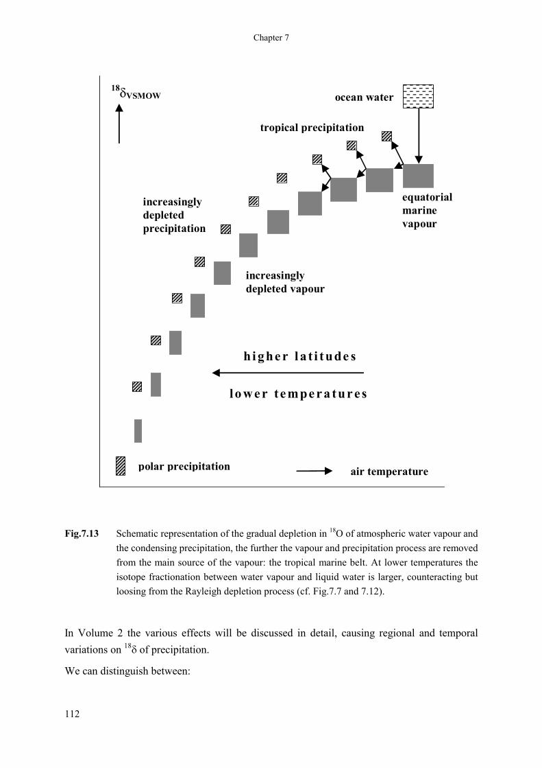
main source of the vapour in the equatorial regions. In the Arctic and Antarctic, 18� of the ice

can be as low as -50‰. This gradual 18O depletion model is schematically shown in Fig.7.13.

111

Chapter 7

equatorialmarinevapour

tropical precipitation

h i ghe r l a t i tude s

lo we r tempe ra tures

polar precipitation

increasinglydepleted vapour

increasinglydepletedprecipitation

ocean water

air temperature

18�VSMOW

Fig.7.13 Schematic representation of the gradual depletion in 18O of atmospheric water vapour and the condensing precipitation, the further the vapour and precipitation process are removed from the main source of the vapour: the tropical marine belt. At lower temperatures the isotope fractionation between water vapour and liquid water is larger, counteracting but loosing from the Rayleigh depletion process (cf. Fig.7.7 and 7.12).

In Volume 2 the various effects will be discussed in detail, causing regional and temporal variations on 18

� of precipitation.

We can distinguish between:

112


1) latitudinal effect with lower 18� values at increasing latitude

2) continental effect with more negative 18� values for precipitation the more inland

3) altitude effect with decreasing 18� in precipitation at higher altitude

4) seasonal effect (in regions with temperate climate) with more negative 18� values during

winter

5) amount effect with more negative 18� values in rain during heavy storms.

7.2.4.3 SURFACE WATER

In Fig.7.8 some data are shown on 18� variations in riverwater. The seasonal variation with

relatively high values in summer is characteristic for precipitation in temperate regions. The basis of both curves represents the average 18

� values of precipitation and groundwater in the recharge areas, i.e. N.W.Europe (Meuse) and Switzerland/S.Germany (Rhine), the latter with a large transport of relatively isotopically light meltwater in spring.

Evaporation, especially in tropical and semi-arid regions, causes 18O enrichment in surface waters. This results, for instance, in 18

� of the river Nile to be +3 to +4‰, and of certain lakes as high as +20‰ (Sect.4.4.5 and 7.5).

7.2.5 CLIMATIC VARIATIONS

The slow precipitation of calcium carbonate is a process during which carbonate and water are in isotopic equilibrium, as was pointed out earlier. The 18O content of the carbonate is, therefore, primarily determined by that of the water. The second determining factor is the temperature, as is indicated in Fig.7.10. Consequently we can in principle deduce the water temperature from 18

� of carbonate samples in marine sediment cores, provided 18� of the

water is known (� 0‰). This was originally believed to be the basis of the 18O palaeothermometry of fossil marine shells (Epstein et al., 1953).

The present-day opinions assume a varying 18� of the surface ocean water during

glacial/interglacial transitions (Emiliani, 1971; Olausson, 1981), due to varying amounts of accumulated ice with low 18

� as polar ice caps. As a realistic order of magnitude, an estimated amount of 5.105 km3 of ice (= Vice) laid down especially on the northern polar ice cap during the last ice age with an average 18

� value of �20 ‰ changes the 18� value (at present = 0 ‰)

of the 107 km3 of ocean water (=Vocean) by +1 ‰, as is simply deduced from the mass balance:

Vpresent ocean� 18�present seawater = Vice-age ocean� 18

�ice-age seawater + Vice caps� 18�ice (7.29)

Another spectacular application of isotope variations in nature is the deduction of climatic changes in the past from 18O/16O or 2H/1H ratios in polar ice cores. If the process of gradual

113

Chapter 7

isotope depletion of precipitation is studied in detail as a function of latitude and thus of air temperature, a relation can be derived (Volume 2) which comes to the temperature dependence:

d18� / dt � +0.7‰ / �C (7.30)

(Dansgaard, 1964; Van der Straaten and Mook, 1983). By this relation it is possible to translate isotope variations into climatic variations during geologic times. Records have been obtained on ice cores from Greenland and the Antarctic, showing the alternation of low-18

� (or low-2

�) and high-18� (or high-2

�) periods, respectively cold and warm periods (Eq.7.30).

18�

Time (103 years BP)

0 20 40 60 80 100 120 140

marine Arctic Antarctic carbonate+1.5 0 �40 �36 �49 �45

Fig.7.14 Palaeotemperature records represented by 18� variations in time in the CaCO3 fraction

from foraminifera shells in deep-sea core sediments (left), in glacier ice of a Northern Greenland glacier (at Summit), and in glacier ice of an Antarctic ice core (at Vostok), respectively from left to right (figure modified from Lorius and Oeschger, 1994). In each record the left side indicates the lower temperatures, for instance, at 20 000 years BP each curve shows the most recent glacial maximum. The upper 10 000 years contain the present warm interglacial, the Holocene.

114


7.3 RELATION BETWEEN 13C AND 18O VARIATIONS IN H2O, HCO3

�, AND CO32�

Differences and the relations between the various natural water-carbonate systems can nicely be displayed by considering both 18

� of the water and 13� of the dissolved bicarbonate.

Fig.7.15 is a schematic representation of three waters of realistic isotopic composition, each provided with the temperature dependent range of calcite precipitated under equilibrium conditions. This figure essentially is a combined graph of Figs.7.5 and 7.12.

From an isotopic point of view, the 4 common types of water are:

1) Seawater, with 18� values around 0‰ (by definition) at present; the carbonate range is

that of recent marine carbonates. Because of changing glacial and interglacial periods the 18� of ocean water varied in the past. Also the 18

� values of marine limestone have increased during the course of geological time, while the 13

� values have essentially remained the same (Veizer & Hoefs, 1976).

2) Ground- and river water, with an arbitrarily chosen value of 18�. In freshwater

bicarbonate 13� generally is around -11 to -12‰. The isotopic compositions of fresh-

water carbonates derived from this water may result from the known equilibrium fractionations (Tables 6.2 and 6.4), in a similar way as is indicated for marine carbonate.

3) Stagnant surface or lake water can be subjected to processes altering the isotopic composition. Provided the water has a sufficient residence time in the basin, isotope exchange will cause the 13C content to reach isotopic equilibrium with atmospheric CO2. Then 13

� equals that in the ocean. Carbonate 13� and 18

� are related to, respectively, HCO3

� and H2O as indicated for the marine values. The 18O content of the water, especially in warmer climates, will change towards less negative or even positive values due to evaporation.

4) Estuarine water has intermediate values of 13�(HCO3

�) or 13�(DIC) and 18

�(H2O), depending on the degree of mixing of the river- and seawater. The latter behaves conservatively, i.e. is only determined by the mixing ratio; 13

�(DIC) also depends on the DIC values of the mixing components. Therefore, the mixing line is generally not straight. The relation with 13

� of the bicarbonate fraction is even more complicated, as the dissociation equilibria change with pH (even the pH does not at all behave conservatively) (Sect.9.5.4).

115

Chapter 7

18�VPDB , 18

�VSMOW (‰)

5 �C

25 �C

0

� 5

�10

0�5�10

exchange with atm. CO2

lake

rivers

evaporation

estuarine mixing of DIC

ocean

H218O / H13CO3

�

Ca13C18O16O2�

13�VPDB (‰)

Fig.7.15 Relation between the natural variations of 13�(HCO3

� and CaCO3) and 18�(H2O and

CaCO3). The graph is essentially a combination of Figs.7.5 and 7.12. Estuarine mixing only results in a straight line between the river and sea values of 13

�DIC, if CT of the components is equal. Because this is rarely the case, the relation between the two members mostly is observed as a slightly curved line. Additionally, 13

�(HCO3�) in

estuaries is not subject to conservative mixing, because the mixing process rearranges the carbonate fractions (Sect.9.5.4). Depending on the residence times of the water at the surface, evaporation and isotope exchange changes the isotopic composition to higher � values.

116


ocean water arctic sea ice marine moisture (sub)tropical precipitation temperate zone ,, polar ice ,, Alpine glaciers Lake Chad wood cellulose temperate peat zone clay minerals

�200 �150 �100 � 50 0 + 502�VSMOW (‰)

Fig.7.16 General view of 2H/1H variations in natural compounds. The ranges are indicative for the majority of materials shown.

7.4 STABLE HYDROGEN ISOTOPES


The chemical element hydrogen consists of two stable isotopes, 1H and 2H (D or Deuterium), with an abundance of about 99.985 and 0.015% and an isotope ratio 2H/1H � 0.00015 (Urey et al., 1932). This isotope ratio has a natural variation of about 250‰, higher than the 13

� and 18� variations, because of the relatively larger mass differences between the isotopes

(Fig.7.16).

As with 18O, high 2H concentrations are observed in strongly evaporated surface waters, while low 2H contents are found in polar ice. Variations of about 250‰ are present in the part of the hydrological cycle to be discussed here.

7.4.2 HYDROGEN ISOTOPE FRACTIONATIONS

The most important hydrogen isotope fractionation is that between the liquid and the vapour phases of water. Under equilibrium conditions water vapour is isotopically lighter (contains less 2H) than liquid water by amounts given in Table 7.6. Fig.7.3 shows some actual isotope ratios of equilibrium systems and the matching 2

� values. The fractionation by diffusion of H2O through air (2

�d) varies between �22.9 ± 1.7‰ (Merlivat, 1978) and �20.4 ± 1.4‰. (unpubl.), slightly more than the value calculated from Eq.3.34 (�16.3‰) (cf. Sect. 7.3.2).

117

Chapter 7

7.4.3 REPORTING 2H VARIATIONS AND THE 2H STANDARD

VSMOW is the standard for 2H/1H as it is for 18O/16O ratios. Values for the absolute 2H/1H ratio of VSMOW and SLAP are reported to be (155.76 ± 0.07)�10�6 and (89.02 ± 0.05)x10�6, respectively, by Hagemann et al. (1970), (155.75 ± 0.08)�10�6 and (89.12 ± 0.07)�10�6 by De Wit et al. (1980), and (155.60 ± 0.12)�10�6 and (88.88 ± 0.18)�10�6 by Tse et al. (1980).

Table 7.5 The stable and radioactive isotopes of hydrogen: practical data for the natural abundance, properties, analytical techniques and standards. Further details are given in Sect.7.4 and 8.3, and in Chapters 10 and 11.

MS=mass spectrometry, PGC=proportional gas counting, LSS=liquid scintillation spectrometry, AMS=accelerator mass spectrometry

1H 2H 3H

natural abundance 0.99985 0.00015 < 10�17

stability stable stable radioactive

natural specific activity < 1.2 Bq/L water

decay mode / daughter �� / 3He

half-life (T1/2) 12.320 ± 0.022 a

decay constant (�) 5.576�10�2/a = 1/18.33 a�1

max. � energy 18 keV

abundance range

in hydrological cycle

250‰ 0 to 10�16

reported as 2� or �2H or �D 3A

in ‰ TU, Bq/L H2O

instrument MS PGC, LSS

analytical medium H2 H2O, C2H6, C6H6

usual standard deviation 0.5‰ 1% at high level

international standard VSMOW NBS-SRM 4361

with absolute value 2H/1H = 0.00015575 3H/1H = 6600 TU

or = 0.780 Bq/g H2O

as of Jan.1, 1988

118


The average 2� value of the secondary standard SLAP on the VSMOW scale (Sect.7.2.3)

consequently is �428.2 ± 0.1‰. Based on these data the 2� value has been defined as: 2

�SLAP / VSMOW = � 428.0‰ (7.33)

No significant difference in 2� has been detected between the original SMOW standard and

VSMOW (IAEA, 1978).

Table 7.6 Hydrogen isotope fractionation in the equilibrium system liquid water (l), water vapour (v), and ice (i); �y / x represents the fractionation of compound y relative to compound x and is approximately equal to 2

�(y) � 2�(x). Values for intermediate temperatures may be

obtained by linear interpolation; T = t (�C) + 273.15 K.

t

�C

2�v/l 1)

(‰)

18�v/l

(‰)

2�v/l / 18

�v/l 2)

0 �101.0 �11.55 8.7

5 � 94.8 �11.07 8.55

10 � 89.0 �10.60 8.4

15 � 83.5 �10.15 8.25

20 � 78.4 � 9.71 8.1

25 � 73.5 � 9.29 7.9

30 � 68.9 � 8.89 7.75

35 � 64.6 � 8.49 7.6

40 � 60.6 � 8.11 7.4

1) Majoube, 1971 :ln2� = �24 844/T2 + 76.248/T � 0.052612 (7.31a)

1/T adjustment :2�v/l = �85 626/T + 213.4‰ (7.31b)

Values at higher temperatures can be obtained from Horita and Wesolowski(1994) 2) The ratios between the fractionations for 18O and 2H at the liquid�vapour equilibrium are

obtained from Majoube (1971). Majoube, 1971 :2

�i/l = + 19.3‰ (at 0�C) (7.32)

Reference and intercomparison water samples are available from the IAEA (Table 11.3). The 2H contents of hydrogen-containing samples are determined by completely converting them to hydrogen gas. Therefore, fundamental problems of isotope fractionation during sample preparation, as with 18O, do not occur; however, the analyses are more troublesome (Sect.10).

119

Chapter 7

Henceforth all 2� values will be reported relative to VSMOW.

More details on the measurement and calculation procedures, and on isotope reference samples are given in Chapter 10.

7.4.4 SURVEY OF NATURAL 2H VARIATIONS

From the foregoing it is evident that some correlation should exist between 2H and 18O fractionation effects. Therefore, in natural waters a relation between 2

� and 18� values is to be

expected. Indeed, the 2� and 18

� variations in precipitation, ice, most groundwaters and non-evaporated surface waters have appeared to be closely related. Therefore, the qualitative discussion given in Sect.7.2.4 for 18

� applies to 2� equally well. The next section is devoted to this relation.

7.5 RELATION BETWEEN 2H AND 18O VARIATIONS IN WATER

If we simply assume that evaporation and condensation in nature occur in isotopic equilibrium, the relation between the 2� and 18

� values of natural waters is determined by both equilibrium fractionations 2�v/l and 18

�v/l. In Table 7.6 the ratio of these factors is presented for the temperature range of 0 � 40oC.

Craig (1961b) and Dansgaard (1964) found a relation between the 2� and 18

� values of precipitation from various parts of the world:

2� = 8 18

� + 10 ‰ (7.34)

This relation, shown in Fig.7.17 has become known as the Global Meteoric Water Line (GMWL) and is characterised by a slope of 8 and a certain intercept with the 2H axis (= the 2� value at 18

� = 0‰). The general relation is of the MWL is:

2� = s�18

� + d (7.35)

where the slope s = 8, as is explained by the ratio between the equilibrium isotope fractionations of hydrogen and oxygen for the rain condensation process (Table 7.6); d is referred to as the deuterium excess (d-excess), the intercept with the 2� axis. In several regions of the world as well as during certain periods of the year and even certain storms the 2

� value is different from 10 ‰, depending on the humudity and temperature conditions in the evaporation region.

The isotopic composition of water vapour over seawater with 2� = 18

� = 0 ‰ vs VSMOW is somewhat lighter than would follow from isotopic equilibrium with the water: the evaporation

120


ocean water

+ 40

0

� 40

� 80

�120

�160

+40 �8 �4�12�16 �20

water vapour in equilibriumat 200C

meteoric water line: 2� = 8 18� + 10 ‰

rain

remainingvapour

marine atmosphericvapour at equator

condensation

2�VSMOW (‰)

18�VSMOW (‰)

Fig.7.17 Relation between natural variations of 18� and 2

� ocean water, atmospheric vapour and precipitation. The black round represents the hypothetical value of water vapour in isotopic equilibrium with ocean water, black square the observed isotopic composition of equatorial marine vapour, originated from the more realistic non-equilibrium fractionation. Marine vapour gradually condenses into precipitation (hatched arrow) with a positive fractionation, leaving the vapour progressively depleted in 18O and 2H (grey arrow) (cf. Fig.7.13).

is a non-equilibrium (partly kinetic) process. However, from the observed vapour composition onward the vapour and precipitation remain in isotopic equilibrium, because the formation of precipitation is likely to occur from saturated vapour (i.e. vapour in physical equilibrium with water). Consequently the 18

� and 2� values both move along the meteoric water line (Eq.7.33).

121

Chapter 7

evaporated water�

2� = 4.5 �18

�

18�VSMOW (‰)

escaping vapour

meteoric water line: 2� = 8 18

� + 10 ‰

arbitrary freshwaters

estuarine mixing

2�VSMOW (‰)

�10 �8 �6 �2�4 0 +2

�80

�60

� 40

� 20

0

+ 20

ocean water

Fig.7.18 Relation between 18� and 2

� for estuarine mixing and for evaporating surface water. Because the evaporation is a non-equilibrium process, isotope fractionations involved are not necessarily related by a factor of 8, as is the equilibrium condensation process, the basis for the meteoric water line (Fig.7.17). As in the preceding figure, the arrows indicate the direction of change of the isotopic composition of the escaping vapour and of the remaining evaporated water.

122


In Volume 3 (Surface Water) certain circumstances will be discussed leading to deviations from the common MWL. For instance, larger values of d are occasionally observed.

Apart from this, deviations occur in evaporating surface waters, showing slopes of 4 to 5 rather than 8. If 2

�o and 18�o denote the original isotopic composition of an arbitrary surface

water, the � values after evaporation are related by:

2� - 2�o � 4.5 (18

� - 18�o) or 2

� � 4.5 18� (7.35)

(Fig.7.18). The release of relatively low-� water vapour to the air results in a increase in � of the remaining water, as illustrated by the model of Sect.4.4.5, here for 2� as well as 18

�.

123

Chapter 7

124

5 natural abundance of the stable isotopes … i/cht_i_07.pdf · 7 natural abundance of the stable...

Documents