137

5 Development of the Water Quality Index (WQI) to Assess Effects of Basin-wide Land-use Alteration on Coastal Marshes of the Laurentian Great LakesPatricia Chow-Fraser

5.1 INTRODUCTION

Development and use of biological indicators to monitor the status and trends of aquatic ecosystems such as streams and rivers (Karr 1981, 1991; Wichert 1995; Wichert and Rapport 1998), lakes (Hughes and Noss 1992) and inland freshwater wetlands (Keddy et al. 1993; Adamus et al. 2001; Weigel 2003) have become routine for many environmental agencies throughout the world (e.g. van Dam et al. 1998; U.S. EPA 2002). The ecological basis for using biological indicators is that the community of plants and animals will refl ect the overall condition or quality of the habitat. Suter (2001) has criticized that the goal of this form of environmental monitoring, which summarizes the overall effects of both natural and human-induced disturbances, is problematic because it does not address the causal relationship between the disturbance and the indicator, or in terms of environmental risk assessment, the measures of effect and the assessment endpoint, respectively.

In many cases, the presumed human-induced disturbance is the associated increase in nutrient and sediment loading from conversion of forests in the watershed into agricultural and urban land (e.g. Field et al. 1996; Müller et al. 1998; Dodson and Lillies 2001; Wang et al. 2001). In other cases, however, site-level disturbances such as proximity to roads and highways (Nelson and Booth 2002; Eyles et al. 2003; Ourso

CONTENTS

5.1 Introduction ..........................................................................................................................................1375.2 Methods ...............................................................................................................................................142

5.2.1 Study Sites .................................................................................................................................1425.2.2 Field Methods ............................................................................................................................1425.2.3 Physical Parameters ..................................................................................................................1435.2.4 Field Processing ........................................................................................................................1435.2.5 Sample Analyses .......................................................................................................................1435.2.6 Land Use Delineation .............................................................................................................. 1445.2.7 Statistical Procedures ............................................................................................................... 144

5.3 Results ..................................................................................................................................................1455.3.1 Derivation of the Water Quality Index .....................................................................................1495.3.2 Using the WQI ..........................................................................................................................1495.3.3 Predictive Models to Generate WQI Scores .............................................................................1535.3.4 Relationship Between WQI and Basin-Wide Land Use ...........................................................1535.3.5 Comparison of WQI with Other Indices ...................................................................................155

5.4 Discussion ............................................................................................................................................1575.5 Conclusions ..........................................................................................................................................161Acknowledgements .........................................................................................................................................161References .......................................................................................................................................................161

C138

TABLE 5.1.

Summary of relationships between stressors and indicators for coastal wetlands presented in chronological order according to numbers that accompany arrows in Fig. 1. Italics indicate that the relationship is not supported by scientific study.

Number Proposed relationship Supporting literature

1 Signifi cant inverse relationship between late summer percent cover of emergent vegetation and mean annual water level of Great Lake

Species-specifi c response to deep and shallow water will give rise to predictable changes in community composition and structure

Williams and Lyon 1997; Chow-Fraser et al. 1998

Wilcox and Meeker 1992; Thiet 2002

1a Recent low water levels encourage establishment of exotic aquatic plants

Hudon 1997; Hudon et al. 2000

2 Seiche effects will affect nutrient dynamics of exposed wetlands

Seasonally disconnected systems through dykes or natural beach barriers can signifi cantly alter water quality within wetlands

Sager et al. 1985;

McLaughlin and Harris 1990;Keough et al. 1999

3 Signifi cant positive correlation between biomass of benthic algae and water-quality degradation

McCormick et al. 2001; McNair and Chow-Fraser 2003

4 Culturally enriched sediment will affect the species composition and richness of submergent vegetation

Smith et al. 2002; Tracy et al. 2003.

5 Culturally enriched sediment will affect the species composition and richness of emergent vegetation

Chow-Fraser et al. 1998; Miao et al. 2000.

6 Water clarity (depth) determines the extent of submergent vegetation colonization

Water quality determines the species richness of submergent macrophytes

Hudon et al. 2000

Crosbie and Chow-Fraser 1999; Lougheed et al. 2001

7 Benthic algae negatively affects the species richness of submergent macrophytes

McNair and Chow-Fraser 2003

8 Signifi cant positive association between submergent aquatic vegetation and wetland-dependent fi sh

Randall et al. 1996; Chow-Fraser et al. 1998; Wei et al. 2003

9 Water quality affects the diversity and species richness of fi sh

Brazner 1997; Seilheimer and Chow-Fraser, unpub. data

10 Loss of emergent vegetation will lead to eventual loss of submergent vegetation

Engel and Nichols 1994; Chow-Fraser et al. 1998

139

11 Community of submergent vegetation will affect zoobenthos (zooplankton and benthic invertebrates) species richness

Chow-Fraser 1998; Burton et al. 1999; Lougheed and Chow-Fraser 2002

12 Community of emergent vegetation will affect distribution of zoobenthos (zooplankton and benthic invertebrates)

McLaughlin and Harris 1990; Chow-Fraser et al. 1998; Euliss et al. 1999

13 Establishment of exotic species (e.g. common carp, zebra mussels, Eurasian milfoil, purple loosestrife, and common reed) can negatively affect the community dynamics of native plants and animals

Brady et al. 1995; Chow-Fraser et al. 1998; Boylen et al. 1999; Mills et al. 1999; Blossey et al. 2001; Tewksbury et al. 2002; Bartsch et al. 2003; Hall et al. 2003; Nalepa et al. 2003; Wilcox et al. 2003

14 There is a signifi cant positive correlation between biomass of carp and water turbidity

Lougheed et al. 1998; Chow-Fraser 1999

14a Removal of carp benefi ts species richness of submergent vegetation

Lougheed et al. 2003; Angeler et al. 2003

15 Signifi cant interactions exist between wetland fi sh and benthic invertebrates

Kohler et al. 1999; Batzer et al. 2000

16 Boating activities will contribute to degraded water quality

---

16a Boating activities will negatively affect the integrity of the fi sh and benthic community

Backhurst and Cole 2000; Arlinghaus et al. 2002; Penczak et al. 2002

17 Point source discharge will contribute to water-quality impairment

Chow-Fraser 1998 and many others

18 Shoreline modifi cation will reduce available fi sh habitat

Randall and Minns 2002; Garland et al. 2002

19 Roadway/highway runoff contribute to water-quality impairment in urban wetlands; amount of paved surfaces was best correlate (negative) with fi sh diversity and IBI

Chow-Fraser et al. 1996; Wang et al. 2001

20 Riparian condition (presence of buffer strip or location of golf courses/cottages/residential property) can alter water quality independently of basin-wide land use

Lammert and Allan 1999; Meador and Goldstein 2003; Houlahan and Findlay 2003

21 Basin-wide land-use affects water quality in streams and wetlands

Harding et al. 1998; Crosbie and Chow-Fraser 1999; Lougheed et al. 2001

Figure 5.1 Relationship diagram linking stressors (shaded boxes with thickened edges) to indicators (clear boxes). See Table 1 for explanation of relationships and supporting literature.

140

141

and Frenzel 2003) or distance to forest cover (Houlahan and Findlay 2003), riparian condition and shoreline development (e.g. Lammert and Allan 1999; Meador and Goldstein 2003), as well as recreational impact (Kashian and Burton 2000; Lewis et al. 2002; Penczak et al. 2002) can have overriding effects on the biotic community in the absence of changes in basin-wide land uses.

For freshwater wetlands, natural disturbances such as inter-annual changes in water levels (Keddy and Reznicek 1986; Wilcox et al. 2002), site-to-site variation in ambient temperature (Anderson and Vondracek 1999; Tangen et al. 2003), and in-stream hydrologic variability (Poff and Ward 1989; Poff and Allan 1995) may also be more infl uential on the composition of the fl ora and fauna than proportion of developed land in the catchment. Finally, remedial actions such as carp exclusion (Lougheed et al. 2003), treatment of sewage effl uent prior to being discharged into wetlands (Chow-Fraser et al. 1998) and water-level management through dyking (McLaughlin and Harris 1990; Thiet 2002) can induce changes in the plant community that are completely unrelated to natural disturbances or land-use changes. While all these stressor categories can potentially produce changes in the biotic community of impacted relative to least-impacted (or “reference”) sites, few if any of these biotic indices can distinguish among disturbance types (Suter 2001; Wilcox et al. 2002). In addition, a biotic index for two reference sites can vary because of natural variability (e.g. hydrologic regime), or an impacted site may have a biotic score that is similar to that of a reference site because of good riparian condition resulting from implementation of best-management practices (e.g. Wang et al. 2003). Indeed, without knowing the relationship between an environmental condition (stressor) and the biological response, it is diffi cult to select appropriate reference areas for a particular study.

Many coastal marshes of the Laurentian Great Lakes, especially those occurring in Lakes Erie and Ontario show obvious signs of degradation because of poor water quality (Smith et al. 1991; Chow-Fraser and Albert 1999; Thoma 1999). Their great ecological, hydrological, educational and recreational value has prompted governments at all levels to make them a priority both for monitoring and impact assessment. To this end, various agency-wide research programs have been implemented in both Canada and the U.S. to develop appropriate environmental indicators that can be applied widely throughout the Great Lakes basin. Because stressors responsible for ecosystem impairment occur at spatial scales that span local to regional extents, a number of indicators (assessment endpoints) can be measured for coastal wetlands, ranging from information measured at the site level to those sensed remotely (airborne or satellite) (Figure 5.1). These stressors can be considered naturally-occurring (represented by box with black background) or human-induced (represented by boxes with grey background), and can vary in terms of how they relate to a number of abiotic and biotic indicators (boxes with clear background).

The scope of this paper only permits me to discuss a subset of all relationships (arrows) in Figure 5.1, but the specifi c details of all proposed relationships together with supporting literature (numbers accompanying arrows) are summarized in Table 5.1. Water-quality impairment for many coastal wetlands of the lower Great Lakes has been attributed to nutrient and sediment inputs from agricultural and urban landscapes (#21; refer to Figure 5.1 and Table 5.1), although for some marshes, point-source pollution from municipal or industrial waste-treatment facilities (#17) and carp bioturbation (#13) have played an equally important role. Regardless of the pollution source, however, the resulting eutrophic and turbid conditions generally lead to a higher biomass of benthic algae (#3), which can reduce the species richness of submergent plants (#6, #7), and which can in turn affect the species richness, species composition and size structure of higher trophic levels (i.e. zooplankton, benthic invertebrates and fi sh (#8, #11 and #15). A direct link should exist between basin-wide land use (e.g. percentage forested, agricultural and urban land) and water-quality conditions in coastal wetlands (Figure 5.1; Table 5.1), although this assumption has not been tested rigorously at a lake-wide scale of all fi ve Great Lakes. In this paper, I will use water-quality data collected from 110 widely distributed wetland complexes (146 wetland-years; Figure 5.2) to develop a “Water Quality Index” (WQI) that can be used to directly test this assumption. Specifi cally, I will investigate if WQI scores can be statistically related to proportion of forested and altered land in wetland catchments. I will show how WQI scores can be used to assess the quality of wetlands in cross-sectional (many wetlands across the basin at one time) as well as longitudinal studies (how Cootes Paradise has changed over an 8-year period (1994-2001) in response to a carp-exclusion program). For a subset of the wetlands, I will also show how the WQI compares with published IBI ranks derived from benthic macroinvertebrate data for wetlands in Lake Huron (Burton et al. 1999) and from fi sh, plant and macroinvertebrate data for wetlands in Lakes Superior, Michigan and Huron (Wilcox et al. 2002). Finally, I will demonstrate the relationship between water quality (WQI scores) and higher trophic levels, including biomass of benthic algae (McNair and Chow-Fraser 2003), and species richness of submergent plants (Lougheed et al.

142

2001). By directly linking biotic indicators to WQI and percentage land use, I will show that the WQI is a reliable indicator of human-induced land use alterations, and that it should be used as an independent means of assessing wetland quality when developing biological indicators.

5.2 METHODS

5.2.1 STUDY SITES

The database used to develop the WQI includes water-quality information from 110 wetlands located throughout all fi ve Great Lakes (Figure 5.2; Appendix 1). Almost all data included here come from samples collected between 1998 and 2002 (early June to end of August), except those for Cootes Paradise which represent years before (1994) and after implementation of a carp-exclusion program (1998, 2000, and 2001; see Lougheed and Chow-Fraser 2002; Lougheed et al. 2004). In total, there were 53 sites from the lower lakes and connecting channels (including the St. Lawrence River (upstream of Cornwall, Ontario, Canada), Lake Ontario, Niagara River, Lake Erie and Lake St. Clair), and 57 from the upper lakes (including Georgian Bay, Lakes Huron, Michigan and Superior). Wetlands were not randomly selected, but were chosen to represent most of the ecologically important eco-reaches identifi ed in Chow-Fraser and Albert (1999) and to ensure that the database included a very large range of land-use and water-quality conditions.

5.2.2 FIELD METHODS

Water samples used for analysis of planktonic algae, primary nutrients and suspended solids were collected in a standardized manner from an open-water site located at least 10 m from the edge of the aquatic vegetation; in certain wetlands, submergent vegetation was present throughout and in those cases, deeper areas that

Figure 5.2 Location of study sites in this study.

143

had minimal submergent vegetation were sampled. This ensured that samples were not contaminated with benthic algae (either epiphytic or periphytic). All water samples were collected with a clean 1-L van Dorn bottle deployed at mid-depth in the open-water areas. Because water depths in the various wetlands ranged from 20 cm to 5.5 m (mean of 1.1m), it was not always necessary or possible to use the Van Dorn sampler; in those instances, water was collected by simply plunging a clean 1-L beaker upside down into the water and quickly inverting it to collect water, taking care that the sediment and plants were not disturbed in the process. Aliquots of this water were immediately measured in triplicate for water turbidity (TURB) with a Hach Portalab turbidimeter. Samples were also stored in 1-L brown (for planktonic chlorophyll-a) or clear acid-washed (for nutrients and suspended solids) polyethylene bottles, and kept in a cooler until they were processed that evening either in the fi eld or at a laboratory.

5.2.3 PHYSICAL PARAMETERS

Temperature (TEMP), conductivity (COND), pH, and dissolved oxygen (DO) were measured with several in situ probes during the study period. Prior to 2000, we used a Hydrolab H20 equipped with a Scout monitor (Hydrolab, Austin, Texas, USA); during 2000 and 2001, we used a Hydrolab Minisonde multi-parameter probe and Surveyor monitor (Hydrolab, Austin, Texas, USA); and in 2002, we used a YSI 6600 multi-parameter probe with YSI 650 display (YSI, Yellow Springs, Ohio, USA). During 2001, we conducted a side-by-side comparison of all three instruments, and found no signifi cant differences with respect to any of the above parameters. Regardless of the instrument used, all sensors were calibrated as indicated by the manufacturers at the beginning of multi-day fi eld trips (up to 8 days). The remoteness of many of our sites from the University laboratory (where calibrations were carried out) precluded daily calibrations during these multi-day sampling trips, even though this would have been desirable. The time of day at which these physical measurements were taken varied from site to site; the earliest measurements were taken close to 09:00 and the latest were taken close to 20:00. Differences in sampling times did not generally affect the parameters of interest, except for DO, which could vary from <4 mg/L in early morning to >10 mg/L in mid-day in very eutrophic sites (Chow-Fraser, unpub. data). Coordinates reported for sites sampled prior to 2000 were obtained from published sources (Crosbie and Chow-Fraser 1999 and Lougheed and Chow-Fraser 2002), whereas after 2000, all sites were georeferenced with either a Trimble GPS unit (4- to 5-m accuracy) attached to the Hydrolab Surveyor or a Garmin GPS unit (4- to 6-m accuracy), which was attached to the YSI 650 display.

5.2.4 FIELD PROCESSING

Sample processing usually took place within six hours of collection. Water for nutrient analyses were dispensed into clean, acid-washed Nalgene bottles that had been fi rst rinsed with deionized water. They were then kept frozen until analysis (usually within three months of collection). Samples for chlorophyll-a content of phytoplankton (CHL) were fi rst fi ltered through 0.45-µm GF/C fi lters, and then stored frozen in tin foil. Parallel samples for total suspended solids (TSS) were similarly fi ltered through pre-weighed fi lters, then placed in clean small petri plates, sealed and put in a freezer.

5.2.5 SAMPLE ANALYSES

At the time of analysis, frozen fi lters designated for CHL analyses were unwrapped from foil, placed in 10 mL of 90% reagent-grade acetone, and kept in the freezer from 4 to 24h (APHA 1992). Samples were then centrifuged, and chlorophyll-a content was determined by measuring absorbance with a Milton Roy 301 spectrophotometer before and after acidifi cation (to account for phaeophytin pigments). Chlorophyll samples reported in this study were all measured in triplicate, and fi nal concentrations were calculated as described in Chow-Fraser et al. (1994). Following digestion in potassium persulfate in an autoclave, samples for total phosphorus (TP) were measured in triplicate according to the molybdenum blue method of Murphy and Riley (1962). Samples for soluble reactive phosphorus (SRP) were fi rst passed through 0.45 µm-fi lters before molybdenum blue analysis, without digestion. Total Kjeldahl nitrogen (TKN), total nitrate nitrogen (TNN) and total-ammonia nitrogen (TAN) (measured on the day of water collection) were processed and analyzed with Hach protocols and reagents (Hach Company 1989) with a Hach DR2000 spectrophotometer (Hach, Loveland, Colorado, U.S.A.). Total nitrogen (TN) was calculated by addition of TKN and TNN.

144

Filters designated for TSS analyses were taken out of the freezer and fi rst dried at 100°C for 1 h, then dried in a dessicator with calcium sulphate for another hour, before they were weighed to determine TSS. Loss on ignition was determined after combustion at 550°C for 20 min, followed by drying in the dessicator for an hour. Weight of the combusted fi lter was assumed to be total inorganic suspended solids (TISS), whereas difference in the weight of the fi lter before and after combustion was total organic suspended solids (TOSS).

5.2.6 LAND USE DELINEATION

I was able to obtain basin-wide land-use information for a subset of the 110 wetlands in two ways. First, I obtained information from published sources (Crosbie and Chow-Fraser 1999; Kashian and Burton 2000; Wilcox et al. 2002). Secondly, I delineated watersheds from topographic maps (1:50,000 and 1:24,000, respectively for Canadian and U.S. wetlands, respectively), and overlaid corresponding land-use information as described in Crosbie and Chow-Fraser (1999). I may have introduced an unknown and probably inconsistent error across the dataset because land-use maps for most of the Canadian wetlands date back to the mid-to-late 1980s, whereas the sampling was carried out in the late 1990s and early 2000s. I do not know the extent to which this bias applies to the U.S. wetlands since published land-use information had not been fully described in these papers. This error was unavoidable because updated land-cover data that can be applied to the entire Great Lakes basin do not currently exist. Since published sources did not uniformly report proportions of all land uses, I was only able to obtain land-use information classifi ed into the three categories (i.e. forested, agricultural or urban) for 45 wetlands. However, when I was willing to examine forested versus altered (lumping agricultural and urban categories together), I was able to calculate proportion of altered land (PROPALT) for 74, and proportion of forested land (PROPFOR) for 81 sites, and this greatly increased the statistical power of my analyses.

5.2.7 STATISTICAL PROCEDURES

I used SAS JMP for the Macintosh (version 4.04; SAS Institute Inc., Cary, North Carolina) to conduct all the univariate analyses (paired

TABLE 5.2.

Summary of water- and sediment-quality variables originally considered in the principal components analysis, and those that were finally included in the development of the WaterQuality Index (WQI).

VariableIncluded in final WQI

model

Depth (cm) No

Turbidity (TURB; NTU) Yes

Temperature (TEMP, °C) Yes

pH Yes

Conductivity (COND; µS/cm) Yes

Dissolved oxygen (DO; mg/L) No

Chlorophyll-a (CHL; µg/L) Yes

Total suspended solids (TSS; mg/L) Yes

Total inorganic suspended solids (TISS; mg/L)

Yes

Total organic suspended solids (TOSS; mg/L)

No

Total phosphorus (TP; µg/L) Yes

Total dissolved phosphorus (TDP; µg/L)

No

Soluble reactive phosphorus (SRP; µg/L)

Yes

Total kjeldahl nitrogen (TKN; µg No

Total ammonium nitrogen (TAN; µg/L)

Yes

Total nitrate nitrogen (TNN; µg Yes

Total nitrogen (TN; µg Yes

TN:TP ratio No

Sediment total phosphorus (TPsed; µg/g)

No

% Inorganic sediment (TISSsed) No

% Organic sediment (TOSSsed) No

145

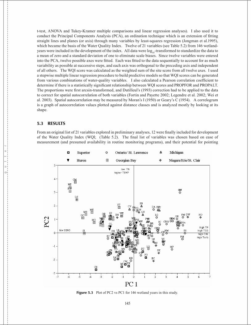
t-test, ANOVA and Tukey-Kramer multiple comparisons and linear regression analyses). I also used it to conduct the Principal Components Analysis (PCA), an ordination technique which is an extension of fi tting straight lines and planes (or axis) through many variables by least-squares regression (Jongman et al.1995), which became the basis of the Water Quality Index. Twelve of 21 variables (see Table 5.2) from 146 wetland-years were included in the development of the index. All data were log10-transformed to standardize the data to a mean of zero and a standard deviation of one to eliminate scale biases. Since twelve variables were entered into the PCA, twelve possible axes were fi tted. Each was fi tted to the data sequentially to account for as much variability as possible at successive steps, and each axis was orthogonal to the preceding axis and independent of all others. The WQI score was calculated as the weighted sum of the site score from all twelve axes. I used a stepwise multiple linear regression procedure to build predictive models so that WQI scores can be generated from various combinations of water-quality variables. I also calculated a Pearson correlation coeffi cient to determine if there is a statistically signifi cant relationship between WQI scores and PROPFOR and PROPALT. The proportions were fi rst arcsin-transformed, and Dutilleul’s (1993) correction had to be applied to the data to correct for spatial autocorrelation of both variables (Fortin and Payette 2002; Legendre et al. 2002; Wei et al. 2003). Spatial autocorrelation may be measured by Moran’s I (1950) or Geary’s C (1954). A correlogram is a graph of autocorrelation values plotted against distance classes and is analyzed mostly by looking at its shape.

5.3 RESULTS

From an original list of 21 variables explored in preliminary analyses, 12 were fi nally included for development of the Water Quality Index (WQI; (Table 5.2). The fi nal list of variables was chosen based on ease of measurement (and presumed availability in routine monitoring programs), and their potential for pointing

Figure 5.3 Plot of PC2 vs PC1 for 146 wetland years in this study.

146

TABLE 5.3.Summary of eigenvalues produced by PCA using standardized values of 12 water-quality variables for 146 wetland-years.

PC axis Eigenvalue Percentexplained

Cumulative Percent explained

1 5.6039 46.699 46.6992 1.5204 12.670 59.3693 1.1218 9.348 68.7184 0.9541 7.951 76.6695 0.7172 5.977 82.6456 0.6255 5.212 87.8587 0.4412 3.677 91.5358 0.3340 2.783 94.3179 0.2726 2.272 96.58910 0.2191 1.826 98.41511 0.1264 1.053 99.46812 0.0638 0.532 100.000

TABLE 5.4.Summary of correlation coefficients between principal components (PC) scores and environmental variables and loadings for each parameter in respective PC axes.

Variance explained (%)

Environmental Variable Loading r-value P-value

PC1 46.69 TPTURB

TSSTISSCHL

COND

0.370560.361750.346460.330310.322170.31942

0.8770.8560.8200.7820.7630.756

0.00010.00010.00010.00010.00010.0001

PC2 12.67 pHTEMP

TN

0.449200.44180

-0.37226

0.5540.545-0.459

0.00010.00010.0001

PC3

Cumulative

9.35

68.71

TEMPpH

COND

----

0.504680.390730.36816

0.5350.4140.390

----

0.00010.00010.0001

----

147

out unique information when included. Dissolved oxygen (DO) was initially included, but was subsequently dropped because this was the only variable that was extremely sensitive to the time of day at which it was measured (see Methods) and since it was not possible to standardize the time of sampling for all sites, a single reading could not be used to represent the full range of DO conditions encountered at that site. A more meaningful indicator of oxygen conditions may be a daily mean calculated from continous hourly measurements (Chow-Fraser, unpub. data).

The twelve variables from 146 wetland-years were entered into the Principal Components Analysis. Although the PCA fi ts as many axes as there are variables, the fi rst four axes explained 76% of all the variation in the dataset (Table 5.3). The fi rst axis, which explained 47% of the total variation, ordinated wetlands according to the degree of water-quality impairment, since it was highly correlated with, TP, TURB, TSS, ISS, CHL and COND (Table 5.4). A plot of the PC1 scores against respective PC2 scores for all wetland-years is a good way to show the ordination results (Figure 5.3). The most degraded wetlands, those that were highly turbid, nutrient-rich, and had high water conductivity (e.g. Old Woman Creek (OW) and Holiday Marsh (HO)) were located at the far right on Axis 1, while the least-impacted wetlands, those that had clear water, low nutrient and low water conductivity (e.g. Cloud Bay (CB) in Lake Superior and Port Rawson (RW), Longuissa Bay (LG) and Sandy Island (SI) in Georgian Bay) were located at the opposite end (Figure 5.3). The second axis, which accounted for an additional 13% of the variation, was signifi cantly correlated with temperature, pH and nitrogen concentrations (Table 5.4; Figure 5.3), which refl ected in part the large geographic distribution of wetlands throughout the fi ve Great Lakes and their associated differences in bedrock geology and latitude. The negative correlation between TN and PC2 is primarily driven by the nutrient-poor sites in Georgian Bay (Moon River Falls (MF) and Cormican Bay (CM)). The third axis was signifi cantly correlated with COND and pH (Table 5.3; Figure 5.4); the Georgian Bay sites with very soft water (Port Rawson (RW), Longuissa

Figure 5.4 Plot of PC3 vs PC1 for 146 wetland years in this study.

148

Figure 5.5 Wetlands with positive WQI scores are presented in descending order of rank. Years associated with the WQI scores appear to the right of the bars.

149

Bay (LG), Cormican Bay (CM) were clustered away from the more alkaline sites that occur in Lake Ontario and Erie (Figure 5.4).

Both PC1 and PC2 were strongly correlated with nutrients and suspended solids (Figure 5.3), and together explained almost 60% of the total variation. These axes effectively ordinated wetlands according to degree of water-quality impairment, regardless of lake of origin. For instance, sites designated by the IJC within Areas of Concern (AOC) (International Joint Commission 2003) in Lake Ontario (Jordan Harbour (JH), Niagara River RAP; Cootes Paradise (CP) and Grindstone Creek (GC; GF), Hamilton Harbour RAP; and Humber River (HM), Toronto and Region RAP) were positioned far to right of the less impacted wetlands in eastern Lake Ontario (Salmon River (SA); Sandy Creek (SC); Weller’s Bay (WB)). Similarly, the degraded wetlands that occur in western Lake Erie (Holiday Marsh (HO) and Old Woman Creek (OW)) occur far to the right of those high-quality wetlands of Long Point Marsh complex (LO, LP, TP). Even though most of the Georgian Bay wetlands were very good quality, AOC sites (Collingwood (CO) and Matchedash Bay (MB)) were positioned to the extreme right of the group. Although there was not as great a range of water-quality impairment for the Lake Superior wetlands, there were similar trends with degraded sites (Mission Island (MI) and Pine Bay (PB)) occurring to the right of pristine sites such as Cloud Bay (CB).

5.3.1 DERIVATION OF THE WATER QUALITY INDEX

In the initial stages of developing the Water Quality Index, I only included the fi rst four axes, since they together explained 76% of the total variability. A reviewer of an earlier draft of this paper argued that I needed to include the fi rst seven, which together explained 90% of the total variation. In the end, I opted to include all twelve axes, rather than risk losing any amount of useful information. Therefore, the Water Quality Index (WQI) score for any wetland was the weighted sum of all PC site scores (i.e. all twelve axes). That is, I multiplied the wetland score associated with a particular PC axis with the proportion of variation explained by the corresponding eigenvalue (i.e. PC1 * 0.46699; PC2 * 0.1267., etc; see Table 5.3), and summing the products for all twelve PC axes for each of the 146 wetland-years.

The highest score (interpreted as being the most pristine) calculated in this dataset was less than +3 (see Figure 5.5), while the lowest score was greater than –3 (interpreted as being the most degraded) (see Figure 5.6). For ease of interpretation, I arbitrarily divided the scale into six categories as follows:

WQI Score Category

+3 to +2+2 to +1

ExcellentVery good

+1 to 0 Good0 to -1-1 to -2

Moderately degradedVery degraded

-2 to -3 Highly degraded

There is no theoretical reason for choosing six categories. It should be considered a starting point, to be revised when a better scheme emerges. Wetlands originating from all fi ve Great Lakes were represented in the “Good” to “Excellent” categories (all positive scores; Figure 5.5), as well as the “Moderately degraded” to “Highly degraded” categories (all negative scores; Figure 5.6). Although there were disproportionately more Georgian Bay wetlands in the good categories (solid bars), the index was able to identify the AOCs (Collingwood and Matchedash Bay (Severn Sound AOC)) as being “Moderately degraded”. By comparison, almost all of the “Very degraded” and “Highly degraded” sites were from Lakes Erie and Ontario, while two wetlands were from Lake Michigan (blue bars), Long Tail Point in Green Bay and Kalamazoo River, which are both associated with AOCs (Figure 5.6).

5.3.2 USING THE WQI

The index was effective in tracking the improved health of Cootes Paradise Marsh, over the course of a marsh-wide carp exclusion program as part of the Hamilton Harbour Remedial Action Plan (Lougheed et al. 2004). In

150

Figure 5.6 Wetlands with negative WQI scores are presented in descending order of rank. Bars corresponding to Cootes Paradise Marsh (Lake Ontario) are indicated by arrows. Years associated with the WQI scores appear to the left of the bars.

151

1994, three years prior to the carp exclusion, the marsh had a very low WQI score, sharing the rank of “Highly degraded” with a handful of other wetlands (Old Woman Creek, Holiday Conservation Area, Grindstone Creek, Jordan Harbour, and Fifteen Mile Creek) (Figure 5.6). In 1998, one year following carp exclusion, the WQI score improved slightly, although it was still found within the “Highly degraded” category. In 2000 and 2001, the corresponding WQI scores continued to increase and placed the marsh in the “Very degraded” category. A key point is that these improvements in water quality have been accompanied by improved health of the zooplankton (Lougheed and Chow-Fraser 2002), plant, and fi sh communities (Lougheed et al. 2004).

To determine if WQI scores varied signifi cantly between years for 23 other wetlands, I used both a paired t-test and a Wilcoxon sign-rank test to compare 1998 WQI scores with those from 2000, 2001 or 2002. There were no signifi cant differences between years (two-tailed t test: P=0.6338, correlation=0.82439; Wilcoxon test: P=0.746), which indicated to me that data were reasonably well replicated through the fi ve years. It confi rmed the robustness of the indicator because the index is based on data collected during a single visit each summer. Of the 23 wetlands, 18 retained the same status, two worsened, while three improved, although it is not clear if these were due to management actions or to natural variation (Table 5.5). Nevertheless, if only 13% of the

TABLE 5.5.Comparison of ranks between 1998 and 2000,2001 or 2002 as determined by WQI scores.

Type of Change Wetland Rank in 1998

Rank in 2000, 2001 or 2002

None Cloud Bay Very good Very goodRondeau Bay Good GoodSpanish River Good GoodTurkey Point Good GoodWellers Bay Good GoodChippewa Park Good GoodEcho Bay Good GoodMadoma Creek Good GoodPresqu’ile Provincial Park Good GoodHay Bay Marsh Good GoodOliphant Bay Good GoodLong Point Big Creek Moderately degraded Moderately degradedMatchedash Bay Moderately degraded Moderately degradedFrenchman’s Bay Moderately degraded Moderately degradedPine Bay Moderately degraded Moderately degradedGrand River Marsh (Dunville) Very degraded Very degradedHumber River Very degraded Very degradedHurkett Cove Good Moderately degraded

Worsened Grindstone Creek Very degraded Highly degradedLittle Cataraqui Creek Good Very degraded

Improved Fifteen Mile Creek Highly degraded Very degradedBronte Creek Very degraded Moderately degradedMission Island Moderately degraded GoodCootes Paradise Marsh Highly degraded Very degraded

152

TABLE 5.6.Summary of regression equations to predict WQI scores

Eq. # Variables in model Associated r2-value

Predictive equation

1 All 12 variables: TURB, TSS, ISS, TPSRP, TAN, TNN, TN, COND, TEMP, pH, CHL

1.00 +10.0239684- 0.3154965 * log TURB-0.3656606 * logTSS -0.3554498 * log ISS -0.3760789 * log TP -0.1876029 * log SRP -0.0732574 * log TAN -0.2016657 * log TNN -0.2276255 * log TN -0.5711395 * log COND-1.1659027 * log TEMP -4.3562126 * log pH -0.2287166 * log CHL

2 TURB, TSS, TP, CONDTN

0.965 +5.2427978 -0.298509 * log TURB-0.865436 * log TSS-0.626229 * log TP -0.818190 * log COND-0.330760 * log TN

3 TURB, COND, TEMP, pH, TP, TN, CHL 0.964 +10.753047-0.946098* log TURB-0.837294 * log COND-1.319621 * log TEMP-4.604864 * log pH-0.387189 * log TP-0.353713 * log TN-0.337888 * log CHL

4 TP, TN, SRP, TNN, TAN, TSS, CHL 0.963 +3.8311461-0.629834 * log TP-0.271059 * log TN-0.083724 * log SRP-0.211261 * log TNN-0.119190 * log TAN-0.995406 * log TSS-0.243290 * log CHL

5 TURB, COND, TEMP, pH, SRP, TNN, TAN

0.947 +11.88597-1.147966 * log TURB-1.048255 * log COND-2.308968 * log TEMP-4.653771 * log pH-0.278112 * log SRP-0.324002 * log TNN-0.116383 * log TAN

153

wetlands examined showed an improvement since 1998, it is probably reasonable to conclude that the positive trend in Cootes Paradise since 1994 refl ects the effects of remedial actions rather than sampling error.

5.3.3 PREDICTIVE MODELS TO GENERATE WQI SCORES

Given that the WQI scores were calculated by summing PCA scores, I carried out a series of stepwise multiple regressions to derive predictive equations with which others could generate WQI scores from raw data (Table 5.6). Besides the 12-variable model that describes the total variation in WQI scores (Eq. 1), there are a number of predictive equations that only require fi ve to seven variables that are commonly collected in routine monitoring programs by environmental agencies. Since the r2-values associated with Eq. 2 to 6 inclusive are uniformly high (0.947 to 0.965), they should generate WQI scores that are comparable to each other. I have included Eq. 7 and 8, even though the associated r2-values are lower (0.90 and 0.85, respectively) because the parameters involved are commonly available.

5.3.4 RELATIONSHIP BETWEEN WQI AND BASIN-WIDE LAND USE

To determine if WQI scores are signifi cantly related to basin-wide land use, I conducted a Pearson correlation analysis. The land use variables I used were PROPFOR and PROPALT, which correspond to the proportion of forested and altered land (combination of both urban and agricultural land), respectively. Because the data were suspected to be spatially autocorrelated, spatial correlograms were used to identify the scales of variation in WQI and the land-use data. The distribution of Moran’s I indicate that the range of infl uence of autocorrelation for both independent variables were similar, at three distance units, while the water quality data were spatially autocorrelated at one distance unit, with one distance unit being approximately 1.3 decimal degrees. Since the data were spatially autocorrelated, Dutilleul’s (1993) correction had to be applied to the data prior to the correlation analysis (Wei et al. 2004). WQI scores were signifi cantly correlated with both arcsin PROPFOR (n=81, r=0.59049, P=0.04763) and arcsin PROPALT (n=64, r=-0.66026, P=0.02295). Had I not corrected for the spatial autocorrelation, the unadjusted P-values associated with the correlation coeffi cients for both would have been <0.0001 and the corresponding r-values would have been 0.64 and 0.72, respectively.

6 TURB, COND, TEMP, pH, TP, TN 0.947 +11.590154-1.073765 * log TURB-0.916011 * log COND-1.684796 * log TEMP-4.677050 * log pH-0.599127 * log TP-0.306512 * log TN

7 TURB, COND, TEMP, pH 0.898 +9.2663224-1.367148 * log TURB-1.577380 * log COND-1.628048 * log TEMP-2.371337 * log pH

8 TP, TN, COND, CHL 0.867 +5.2333056-0.832012 * log TP-0.313032 * log TN-0.982628 * log COND-0.583014 * log CHL

9 TP, TAN, TNN, TN, CHL 0.853 +3.5161294-0.985870 * log TP-0.195332 * log TAN-0.261192 * log TNN-0.171508 * log TN-0.599259 * log CHL

Figure 5.7 Relationship between WQI scores and a) arcsin proportion forested land (n=81) and b) arcsin proportion altered land (n=74). Data for Cootes Paradise (CP) from 1994 to 2001 are indicated.

154

155

Since both relationships were signifi cant even after correcting for spatial autocorrelation, I plotted WQI scores against arcsin PROPFOR and arcsin PROPALT to provide a means of predicting water-quality conditions from basin-wide land use information. Rather than fi tting a straight line through the PROPFOR data, I obtained a better fi t with a logarithmic regression (Figure 5.7a). If we assume that only negative WQI scores indicate degraded conditions, then the minimum amount of forested land in the watersheds should not drop below arcsin proportion of 0.50 (interpolated from the y-axis to the x-axis), which is approximately 48%. By comparison, the infl uence of developed land on water quality appears to be linear, indicating that there is no threshold effect (Figure 5.7b). Data for Cootes Paradise are indicated in both panels, and confi rm that management actions can effect substantial changes in water-quality conditions, irrespective of basin-wide changes in land use. Improved riparian conditions through provision of buffer strips (e.g. Snyder et al. 2003) probably account for some of the high WQI scores above the best-fi t line in Figure 5.7a and b, and future research should be devoted to this line of inquiry.

I regrouped the data into four categories based on dominant land use in the wetland catchment: mainly forested, mixed land-use development, mainly urban, or mainly agricultural (Figure 5.8). The was an uneven distribution among the four categories, with many more agricultural watersheds than any of the other types. Not surprisingly, mean WQI scores for the mostly undeveloped watersheds (forested) were highest, and the mean was not signifi cantly different from that of wetlands with mixed development (where the combined percentage of altered land did not exceed 50%). This is consistent with the earlier observation that good water-quality conditions tended to be maintained as long as the percentage of undeveloped land in the watershed remained above 50% (Figure 5.7a). Wetlands in primarily agricultural watersheds yielded the lowest mean WQI score (-1.009), and this was signifi cantly lower than the primarily urbanized wetlands, which had a mean WQI score of –0.2062.

5.3.5 COMPARISON OF WQI WITH OTHER INDICES

With the recent interest in indices development, I was able to assemble published information to compare with my ranks for 9 of the wetlands (Table 5.7). Five of these sites were ranked in more or less the same way in the published source as they were in this study (Bark Bay, Pentwater River, Mackinaw Bay, Mismer Bay and Wild Fowl Bay). However, for four of the wetlands, there were some notable differences. The greatest deviation was found for Matchedash Bay, which had been ranked by Minns et al. (1994) as being 68% “Good” and 24% “Fair”, but which was ranked in this study as being moderately degraded in all three years of sampling (1998, 2002, and 2003). One reason for this disparity may be that Minns et al’s data had been collected over a decade earlier (1990), and environmental conditions in the marsh have since deteriorated. An alternate explanation is that the

two studies do not share the same reference point, and hence, conditions considered moderately degraded in this study had been deemed to be good in theirs.

There were three other discrepancies in Table 5.7 that should be pointed out. The two Lake Michigan wetlands, Betsie and Lincoln River, were ranked as “Good” in Wilcox et al.’s study, but were ranked as “Moderately degraded” in this study. Another difference is that Betsie and Lincoln had identical total IBI scores (82; Table 9 in Wilcox et al. 2002), whereas in this study, Betsie had a substantially higher WQI score than did Lincoln (Figure 5.6). Unfortunately, without more site-specifi c information, it is virtually impossible to determine which index produced the more accurate assessment.

The last wetland I will mention is Cedarville, which had been identifi ed

Figure 5.8 Comparison of mean WQI scores for various land-use categories. Similar letters indicate that means are statistically homogeneous (ANOVA: P<0.0001; Tukey-Kramer multiple comparisons P>0.05). Numbers indicate the number of wetlands in each category.

156

TABL

E 5.

7.C

ompa

riso

n of

rank

s de

term

ined

by

vari

ous

indi

ces

for s

ubse

t of c

oast

al m

arsh

es in

this

stu

dy.

Rank

s th

at a

re in

bol

d in

dica

te th

at ra

nks

assi

gned

to

wet

land

s di

ffer

ed b

etw

een

stud

ies.

Lake

Wet

land

Sour

ceIn

dex

used

Rank

Supe

rior

Bar

k B

ayW

ilcox

et a

l. 20

02Pl

ant,

Fish

, Inv

erte

brat

e IB

IG

ood

Thi

s stu

dyW

QI

Goo

d

Mic

higa

nB

etsi

e R

iver

Wilc

ox e

t al.

2002

Plan

t, Fi

sh, I

nver

tebr

ate

IBI

Goo

dT

his s

tudy

WQ

IM

oder

atel

y de

grad

ed

Lin

coln

Riv

erW

ilcox

et a

l. 20

02Pl

ant,

Fish

, Inv

erte

brat

e IB

IG

ood

Thi

s stu

dyW

QI

Mod

erat

ely

degr

aded

Pent

wat

er R

iver

Wilc

ox e

t al.

2002

Plan

t, Fi

sh, I

nver

tebr

ate

IBI

Poor

Thi

s stu

dyW

QI

Poor

Hur

onC

edar

ville

Bay

Bur

ton

et a

l. 19

99In

vert

ebra

te I

BIM

oder

atel

y de

grad

ed

Thi

s stu

dyW

QI

Goo

d

Mac

kina

w B

ayB

urto

n et

al.

1999

Inve

rteb

rate

IBI

Mild

ly im

pact

ed

Thi

s stu

dyW

QI

Goo

d/M

oder

atel

y de

grad

edM

ism

er B

ayB

urto

n et

al.1

999

Inve

rteb

rate

IBI

Ref

eren

ce C

ondi

tion

Thi

s stu

dyW

QI

Goo

d

Wild

Fow

l Bay

Bur

ton

et a

l. 19

99In

vert

ebra

te I

BIM

ildly

impa

cted

Thi

s stu

dyW

QI

Mod

erat

ely

degr

aded

Geo

rgia

n B

ayM

atch

edas

h B

ayM

inns

et a

l. 19

94T

his s

tudy

Fish

IBI

WQ

IG

ood-

Fair

Mod

erat

ely

degr

aded

158

equipment. As is true for any index, parameters included in an initial derivation can be deleted and other more useful parameters added in subsequent versions. Therefore, the WQI may need to be modifi ed to account for the effect of water colour, especially when assessing dystrophic wetlands of upper Georgian Bay, where reduced light availability does not necessarily refl ect anthropogenic impact.

One of the major criticisms levied against the use of biotic indices to detect the effect of human disturbance in coastal wetlands is that the target communities (fi sh, macroinvertebrates, plants) are often simultaneously responding to other natural stressors such as water level in addition to anthropogenic impacts (see Figure 5.1), and hence, the resulting IBI scores may lead to erroneous conclusions (Wilcox et al. 2002). In the case of the Laurentian Great Lakes, differences in regional climatic conditions (Minc 1997) may also mask any effect of human disturbance when the indicator is applied throughout the basin (Seilheimer and Chow-Fraser unpub. data). Here, I am not arguing against the use of biological indicators per se, but rather I argue for more effort to be put towards developing indicators (chemical, physical or biological) that can be linked to a well-defi ned stressor, rather than to developing indicators of overall biological/community health (Goldstein et al. 2002).

The strength of a large-scale approach such as that used in this study is that managers have an opportunity to scale and rank wetlands in their jurisdiction against those that occur throughout the Great Lakes basin. But even if managers responsible for wetlands in Lake Erie and Ontario are not interested in comparing their wetlands

with those in Lake Superior, they can use the WQI to rank wetlands on a lake-by-lake basis. Wetlands sampled in the two lower Great Lakes were found in all except the “excellent” category (Figure 5.11), and this confi rms the general applicability of the WQI on both a regional and basin-wide scale. If they need to establish a more locally relevant ranking system, managers could use biotic indices such as the Wetland Zooplankton Index (Lougheed and Chow-Fraser 2002) to resolve small changes in food-webs resulting from site-level impacts that are not related to landscape-level alterations. Further effort should be devoted to documenting the relationship between biotic indices and the water-quality index so that individual metrics that are diagnostic of water-quality impairment can be identifi ed.

Many recent investigators have identifi ed the conversion of forested land in watersheds to be a primary cause of water-quality impairment in freshwater ecosystems (Field et al. 1996; Müller et al. 1998; Crosbie and Chow-Fraser 1999; Nelson and Booth 2002;

0

5

10

15

20

25

-3 -2 -1 0 1 2 3

y = 3.916x + 9.530r2 = 0.594 n = 87P<0.0001

Michigan

Georgian Bay

Huron

Niagara/Erie/St. Clair

St. Lawrence/Ontario

CO

ST

WEKE

ME

MO

GC

SI

MR

CM

RW

MF

0

5

10

15

20

25

-3 -2 -1 0 1 2 3

WQI score

y = 2.374x + 5.616r2 = 0.156 n = 44P=0.008

Superior

Michigan

Georgian Bay

Huron

CWCW

spec

ies

richn

ess

of s

ubm

erge

nts

WQI score

Above 45 No

Below 45 No

Figure 5.10 Relationship between species richness of submergent aquatic vegetation and WQI scores for two groups of wetlands, according to their location south or north of the 45°N Latitude.

Figure 5.11 WQI scores of Lakes Ontario and Erie in descending order of quality.

159

160

Houlahan and Findlay 2003). Others have noted that naturalized shorelines and presence of buffer strips can offset the delivery of nutrients and sediments into streams from altered landscapes (Lammert and Allan 1998; Meador and Goldstein 2003). This study is one of the largest efforts in linking water-quality impairment to basin-wide land use for Great Lakes coastal wetlands. Although there were potentially 110 wetlands that could have been included in the analysis, there was incomplete land-cover information and only 81 wetlands were included in the fi nal correlation analysis of proportion of forested land (Figure 5.7a) and 74 for proportion of altered land (Figure 5.7b). The lack of current land-cover data for both Canada and the United States also meant that outdated land-use maps had to be used in many instances, and this probably contributed to the considerable scatter in Figure 5.7. Despite these errors, however, the relationships between water-quality condition and land use were robust, and could be applied to all fi ve Great Lakes. I want to emphasize the importance of using appropriate spatial scale to examine the effects of basin-wide land use because on a lake-by-lake basis, land-use effects would not have been signifi cant for any of the upper lakes (L. Michigan, Huron and Superior) due to the restricted range in land use type. One of the management implications of these results is that watersheds should maintain at least 50% forested land to ensure that water quality does not become degraded (Figure 5.7a). On the other hand, the linear decline in WQI scores with increasing proportion of altered land suggests that the same deleterious effect on water quality would apply regardless of the proportion of land that is already developed (Figure 5.7b). Future studies should focus on determining possible thresholds of impervious areas such as that found for Alaskan streams (Ourso and Frenzel’s 2003). The data should also be re-examined with higher-resolution spatial information to determine ameliorating effects of buffer strips on downstream water quality in these coastal wetlands, and to differentiate among effects of different agricultural enterprises (soya versus corn, dairy production versus intensive hog farming, etc.).

This study also provided a rare opportunity to examine how water quality changed over the course of a restoration project, in the absence of substantial changes in basin-wide land use. In additon to nutrient and sediment enrichment from non-point sources, Cootes Paradise Marsh had also been degraded by a number of other stressors, including disturbance by the common carp (Cyprinus carpio), wind and wave resuspension, and discharge from a wastewater treatment facility (Chow-Fraser et al. 1998). Since carp disturbance was deemed to be one of the primary causes of marsh degradation (Chow-Fraser 1998), the restoration plan included a large-scale carp exclusion that eventually removed 90% of the carp in the marsh (Lougheed et al. 2004). Prior to the carp exclusion in1997 that removed close to 90% of the carp, the WQI score for Cootes Paradise indicated that the marsh was “Highly degraded” (CP94) (Figure 5.7). The fi rst year after the biomanipulation, water-quality conditions improved only slightly (CP98), but within the next four years (CP00 and CP02), the WQI score had increased from –2.20 to –1.06, indicating that the marsh was approaching the “moderately degraded” state. This type of water-quality improvement was accompanied by an increase in the species richness of the submergent community from 1 in 1994 to 7 in 1998. Unfortunately, when water levels remained low during the summer of 1999, many of the submergent species died back, and the emergent community has colonized much of the submergent habitat since that time (Chow-Fraser 2004). This points out the diffi culty in using biotic indicators to track remedial actions in the presence of overriding effects of natural stressors such as extreme interannual water-level fl uctuation.

Like all primary producers, one of the main determinants of macrophyte growth is availability of primary nutrients. Since aquatic plants obtain nutrients from both sediments and the water column, the nutrient content of the water can help determine the species composition and productivity of the wetland (Wisheu et al., 1992), especially when the substrate is naturally impoverished due to basin geology. In some of the Georgian Bay wetlands, where water is dystrophic, the extremely low TP and TN concentrations may limit the diversity of the plant community to only a few highly competitive species. When these wetlands occur in recreational lakes, increased nutrient loading from human activities, however, would tend to increase the species diversity and richness of the aquatic-plant community. This may explain why there were many more submergent species in Sturgeon Bay (ST) compared with Moon River (MR) or Sandy Island (SI) (Figure 5.9b) since the former is a heavily used recreational lake with a well developed cottage community and various campgrounds along the shoreline, whereas the latter two are essentially undeveloped. This apparent inverse relationship between species richness and WQI scores for the Georgian Bay wetlands is consistent with the observed increase in diversity of vascular plants along an upstream-downstream nutrient gradient of a weakly mineralized stream (Thiébaut and Muller 1998) and lakes with low alkalinity (Vestergaard et al. 2000). Thiébaut and Muller (1998) also demonstrated that the species composition of the downstream sites changed from one indicative of oligotrophic to one indicative of eutrophic conditions.

161

The WQI proved to be a valuable indicator of basin-wide land-use effects. It has the power to rank wetlands according to water quality across the entire Great Lakes basin, and was able to produce results that were generally consistent with published biotic indicators. It is suffi ciently sensitive to track changes within a site over the course of a marsh restoration project, and permitted a direct link between improved water quality and removal of carp from Cootes Paradise Marsh. The index is also robust, because it was well replicated between years for 18 of 23 wetlands examined between 1998 and 2002. Water Quality Index scores can be generated from a variety of multiple-regression equations, involving as few as fi ve fi eld variables. I believe the WQI is an effective indicator of human-induced land-use alterations, and suggest that future investigations use this abiotic indicator to help develop their biotic indices.

5.5 CONCLUSIONS

Many factors contribute to water-quality impairment in coastal wetlands of the Great Lakes. Among these are non-point source inputs of sediment and nutrient from agricultural and urban runoff, point-source pollution from municipal or industrial waste-treatment facilities, and carp bioturbation. Regardless of the pollution source, the resulting eutrophic and turbid conditions generally lead to a higher biomass of benthic algae, which can reduce the species richness of submergent plants, and which can in turn affect the species richness, species composition and size structure of higher trophic levels. In this paper, I use water-quality data collected from 110 widely distributed wetland complexes (146 wetland-years) to develop a “Water Quality Index” (WQI). The WQI scores were then statistically related to proportion of forested and altered land in wetland catchments and these scores were used to rank the degree of water-quality impairment in all 110 wetlands across the Great Lakes basin, and to track changes in Cootes Paradise Marsh over an 8-year period (1994-2001) before and after a carp-exclusion program. For a subset of wetlands, WQI scores compared well with published IBI ranks derived from benthic macroinvertebrate, plant and fi sh data. There was a signifi cant positive association between water quality (WQI scores) and higher trophic levels, including biomass of benthic algae and species richness of submergent plants. By directly linking biotic indicators to WQI and percentage land use, I show that the WQI is a reliable indicator of human-induced land use alterations, and should provide an independent and objective means of assessing anthropogenic impacts when developing indices of biotic integrity.

ACKNOWLEDGEMENTS

I thank all the students and volunteers who assisted in collecting, processing and analyzing the water-quality samples. They are too numerous to name here, but you know who you are. An earlier draft of the manuscript benefi ted from discussions with Anhua Wei, Sheila McNair and Titus Seilheimer, and I am especially grateful to Bob Goldstein for providing a balanced review and making suggestions for improvement. I acknowledge the fi nancial support of the Great Lakes Fishery Commission, the Ontario Ministry of Natural Resources under the Canada-Ontario Agreement, and the Natural Sciences and Engineering Research Council of Canada. Anhua Wei assisted with the GIS and spatial autocorrelation analysis.

REFERENCES

Adamus, P., T.J. Danielson, and A. Gonyaw. 2001. Indicators for monitoring biological integrity of inland, freshwater wetlands. A survey of North American Technical Literature (1990-2000). EPA843-R-01. U.S. Environmental Protection Agency, Offi ce of Water, Wetlands Division, Washington, D.C.

Anderson, D.J. and B. Vondracek. 1999. Insects as indicators or land use in three ecoregions in the prairie pothole region. Wetlands, 19, 648-664.

Angeler, D.G., P. Chow-Fraser, M.A. Hanson, and S. Sanchez-Carrillo. 2003. Biomanipulation: a useful tool for freshwater wetland mitigation? Freshwater Biology (In press).

APHA (American Public Health Association), American Water Works Association, and Water Environment Federation. 1992. Standard methods for examination of water and wastewater 18th edition. APHA, Washington D.C.

162

Arlinghaus, R., C. Engelhardt, A. Sukhodolov, and C. Wolter. 2002. Fish recruitment in a canal with intensive navigation: implications for ecosystem management. Journal of Fish Biology, 61, 1386-1402.

Backhurst, M.K. and R.G. Cole. 2000. Biological impacts of boating at Kawau Island, north-eastern New Zealand. Journal of Environmental Management, 60, 239-251.

Bartsch, L.A., W.B. Richardson, and M.B. Sandheinrich. 2003. Zebra mussels (Dreissena polymorpha) limit food for larval fi sh (Pimphales promelas) in turbulent systems: a bioenergetics analysis. Hydrobiologia, 495, 59-72.

Batzer, D.P., C.R. Pusateri, and R. Vetter. 2000. Impacts of fi sh predation on marsh invertebrates: direct and indirect effects. Wetlands, 20, 307-312.

Blossey, B., L.C. Skinner, and J. Taylor. 2001. Impact and management of purpose loosestrife (Lythrum salicaria) in North America. Biodiversity and Conservation, 10, 1787-1807.

Boylen, C.W., L.W. Eichler, and J.D. Madsen. 1999. Loss of native aquatic plant species in a community dominated by Eurasian watermilfoil. Hydrobiologia, 415, 207-211.

Brady, V.J., B.J. Cardinale, and T.M. Burton. 1995. Zebra mussels in a coastal marsh: the seasonal and spatial limits of colonization. Journal of Great Lakes Research, 21, 587-593.

Brazner, J. 1997. Regional, habitat, and human development infl uences on coastal wetland and beach fi sh assemblages in Green Bay, Lake Michigan. Journal of Great Lakes Research, 23, 36-51.

Burton, T.M., D.G. Uzarski, J.P. Gathman, J.A. Genet, B.E. Keas, and C.A. Stricker. 1999. Development of a preliminary invertebrate index of biotic integrity for Lake Huron coastal wetlands. Wetlands, 19, 869-882.

Chow-Fraser, P., D.O. Trew, D. Findlay, and M. Stainton. 1994. A test of hypotheses to explain the sigmoidal relationship between total phosphorus and chlorophyll a concentrations in Canadian lakes. Canadian Journal of Fisheries and Aquatic Sciences, 51, 2052-2065.

Chow-Fraser, P. 1998. A conceptual ecological model to aid restoration of Cootes Paradise Marsh, a degraded coastal wetland of L. Ontario, Canada. Wetland Ecology and Management, 6, 43-57.

Chow-Fraser, P. 1999. Seasonal, interannual and spatial variability in the concentrations of total suspended solids in a degraded coastal wetland of L. Ontario. Journal of Great Lakes Research, 25, 799-813.

Chow-Fraser, P. 2004. Ecosystem response to changes in water level of Lake Ontario marshes:lessons from the restoration of Cootes Paradise Marsh. Hydrobiologia (in press).

Chow-Fraser, P., B. Crosbie, D. Bryant and B. McCarry. 1996. Potential contribution of nutrients and polycyclic aromatic hydrocarbons from the creeks of Cootes Paradise Marsh. Water Quality Research Journal Canada, 31, 485-503.

Chow-Fraser, P. and D. Albert. 1999. Identifi cation of Eco-Reaches of Great Lakes Coastal Wetlands that have high biodiversity values. Discussion paper for SOLEC ’98. Environment Canada and US EPA, Great Lakes National Program Offi ce, Chicago, IL.

Chow-Fraser, P., V.L. Lougheed, B. Crosbie, V. LeThiec, L. Simser, and J. Lord. 1998. Long-term response of the biotic community to fl uctuating water levels and changes in water quality in Cootes Paradise Marsh, a degraded coastal wetland of L. Ontario. Wetland Ecology and Management, 6, 19-42.

Crosbie, B. and P. Chow-Fraser. 1999. Percent land use in the watershed determines the water- and sediment-quality of 21 wetlands in the Great Lakes basin. Canadian Journal of Fisheries and Aquatic Sciences, 56, 1781-1791.

Dodson, S.I., and R.A. Lillie. 2001. Zooplankton communities of restored depressional wetlands in Wisconsin, USA. Wetlands, 21, 292-300.

Dutilleul, P. 1993. Modifying the t-test for assessing the correlation between two spatial processes. Biometrics, 49, 305-314.

Engel, S. and Nichols, S.A. 1994. Aquatic macrophyte growth in a turbid windswept lake. Journal of Freshwater Ecology, 9, 97-109.

Euliss N.H., D.A. Wrubleski, and D.M. Mushet. 1999. Infl uence of agriculture on aquatic invertebrate communities of temporary wetlands in the prairie pothole region of North Dakota, U.S.A. Wetlands, 19, 578-583.

163

Eyles, N., M. Doughty, J.L. Boyce, M. Meriano, and P. Chow-Fraser. 2003. Geophysical and sedimentological assessment of urban impacts in a Lake Ontario watershed and lagoon: Frenchman’s Bay, Pickering, Ontario. Geoscience Canada. (In press).

Field, C.K., P.A. Siver, and A.-M. Lott. 1996. Estimating the effects of changing land use patterns on Connecticut Lakes. Journal of Environmental Quality, 25, 325-333.

Fortin, M.-J. and S. Paytte. 2002. How to test the signifi cance of the relation between spatially autocorrelated data at the landscape scale: a case study using fi re and forest map. Ecoscience, 9, 213-218.

Garland, R.D., K.F. Tiffan, D.W. Rondorf, L.O. Clark. 2002. Comparison of subyearling fall chinook salmon’s use of riprap revetments and unaltered habitats in Lake Wallula of the Columbia River. North American Journal of Fisheries Management, 22, 1283-1289.

Geary, R.C. 1954. The contiguity ratio and statistical mapping. Incorp. Statist., 5, 115-145.Goldstein, R., L. Wang, T.P. Simon, and P.M. Stewart. 2002. Development of a stream habitat

index for the Northern Lakes and Forests Ecoregion. North American Journal of Fisheries Management, 22, 452-464.

Hall, S.R., M.K. Pauliukonis, E.L. Mills, L.G. Rudstam, G.P. Schneider, S.J. Lary, and F. Arrhenius. 2003. A comparison of total phosphorus, chlorophyll a, and zooplankton in embayment, nearshore and offshore habitats of Lake Ontario. Journal of Great Lakes Research, 29, 54-69.

Harding, J.S., Benfi eld, E.F., Bolstad, P.V., Helfman, G.S. and Jones, E.B.D. III. 1998. Stream biodiversity: the ghost of land use past. Proceedings of the National Academy of Science, 95, 14843-14847.

Houlahan, J.E. and Findlay, C.S. 2003. The effects of adjacent land use on wetland amphibian species richness and community composition. Canadian Journal of Fisheries and Aquatic Sciences, 60, 1078-1094.

Hudon, C. 1997. Impact of water level fl uctuations on St. Lawrence River aquatic vegetation. Canadian Journal of Fisheries and Aquatic Sciences, 54, 2853-2865.

Hudon, C., Lalonde, S. and Gagon, P. 2000. Ranking the effects of site exposure, plant growth form, water depth, and transparency on aquatic plant biomass. Canadian Journal of Fisheries and Aquatic Sciences, 57 (Suppl. 1), 31-42.

Hughes, R.M. and Noss, R.F. 1992. Biological diversity and biological integrity: current concerns for lakes and streams. Fisheries, 17, 11-19.

International Joint Commission. 2003. Status of Restoration Activities in Great Lakes Areas of Concern. Final Report. 47 pp. http://www.ijc.org/php/publications/html/aoc_rep/english/report/index.html

Jongman, R.H.G., ter Braak, C.J.F. and van Tongeren, O.F.R. 1995. Data analysis in community and landscape ecology. Cambridge University Press, 299 pp.

Karr, J.R. 1981. Assessment of biotic integrity using fi sh communities. Fisheries 6: 21-27.Karr, J.R. 1991. Biological integrity: a long-neglected aspect of water resource management.

Ecological Applications 1: 66-84.Kashian, D.R. and Burton, T.M. 2000. A comparison of macroinvertebrates of two Great Lakes

coastal wetlands: testing potential metrics for an index of ecological integrity. Journal of Great Lakes Research, 26, 460-481.

Keddy, P.A. and Reznicek, A.A. 1986. Great Lakes vegetation dynamics: the role of fl uctuating water levels and buried seeds. Journal of Great Lakes Research, 12, 25-36.

Keddy, P.A., Lee, H.T. and Wisheu, I.C. 1993. Choosing indicators of ecosystem integrity: wetlands as a model system. In: Woodley, S., Kay, J. and Francis, G. (Eds). Ecological Integrity and the Management of Ecosystems. St. Lucie Press. p. 61-79.

Keough, J.R., Thompson, T.A., Guntenspergen, G.R., and Wilcox, D.A. 1999. Hydrogeomorphic factors and ecosystem responses in coastal wetlands of the Great Lakes. Wetlands, 19, 821-834.

Kohler, S.L., Corti, D., Slamecka, M.C. and Schneider, D.W. 1999. Prairie Floodplain Ponds: Mechanisms affecting invertebrate community structure. Pp. 711-730. In D.P. Batzer, R.B. Rader, and S.A. Wissinger (Eds.). Invertebrates in Freshwater Wetlands of North America: Ecology and Management. John Wiley and Sons, Inc., New York, NY.

164

Lammert, M. and Allan, J.D. 1999. Assessing biotic integrity of streams: effects of scale in measuring the infl uence of landuse/cover and habitat structure on fi sh and macroinvertebrates. Environmental Management, 23, 257-270.

Legendre, P., Dale, M. R. T., Fortin, M.-J., Gurevitch, J., Hohn, M. and Myers, D. 2002. The consequences of spatial structure for the design and analysis of ecological fi eld surveys. Ecogragphy, 25, 601-615.

Lewis, M.A., Boustany, R.G., Dantin, D.D., Quarles, R.L., Moore, J.C. and Stanley, R.S. 2002. Effects of a coastal golf complex on water quality, periphyton and seagrass. Ecotoxicology and Environmental Safety 53: 154-162.

Lougheed, V.L. and P. Chow-Fraser. 1998. Factors that regulate the community structure of a turbid, hypereutrophic Great Lakes wetland. Canadian Journal of Fisheries and Aquatic Sciences, 55, 150-161.

Lougheed, V.L., and Chow-Fraser, P. 2001. Spatial variability in the response of lower trophic levels after carp exclusion from a freshwater marsh. Journal of Aquatic Ecosystem Stress and Recovery, 9, 21-34.

Lougheed, V.L. and Chow-Fraser, P. 2002. Development and use of a zooplankton index to monitor wetland quality in the Laurentian Great Lakes basin. Ecological Applications, 12, 474-486.

Lougheed, V.L., B. Crosbie and P. Chow-Fraser. 1998. Predictions on the effect of carp exclusion on water quality, zooplankton and submergent macropytes in a Great Lakes wetland. Canadian Journal of Fisheries and Aquatic Sciences, 55, 1189-1197.

Lougheed, V.L., Crosbie, B. and Chow-Fraser, P. 2001. Primary determinants of macrophyte community structure in 62 marshes across the Great Lakes basin. Canadian Journal of Fisheries and Aquatic Sciences, 58, 1603-1612.

Lougheed, V.L., Theÿsmeÿer, T., Smith, T. and Chow-Fraser, P. 2004. Carp exclusion, food-web interactions and the restoration of Cootes Paradise Marsh. Journal of Great Lakes Research, 30, 44-57.

McCormick, P.V., M.B. O’Dell, R.B.E. Shuford, J.G. Backus, and W.C. Kennedy. 2001. Periphyton respones to experimental phosphorus enrichment in a subtropical wetland. Aquatic Botany, 71, 119-139.

McLaughlin, D.B. and Harris, H.J. 1990. Aquatic insect emergence in two Great Lakes marshes. Wetlands Ecology and Management, 1, 111-121.

McNair, S.A. and Chow-Fraser, P. 2003. Change in biomass of benthic and planktonic algae along a disturbance gradient for 24 Great Lakes coastal wetlands. Canadian Journal of Fisheries and Aquatic Sciences, 60, 676–689.

Meador, M.R. and Goldstein, R.M. 2003. Assessing water quality at large geographic scales: relations among land use, water physicochemistry, riparian condition, and fi sh community structure. Environmental Management 31: 504-517.

Miao, S., Newman, S. and Sklar, F.H. 2000. Effects of habitat nutrients and seed sources on growth and expansion of Typha domingensis. Aquatic Botany, 68, 297-311.

Mills, E.L., Chrisman, J.R., Baldwin, B., Owens, R.W., O’Gorman, R., Howell, T., Roseman, E.F., and Raths, M.K. 1999. Changes in the dreissenid community in the lower Great Lakes with emphasis on southern Lake Ontario. Journal of Great Lakes Research, 25, 187-197.

Minc, L.D. 1997. Great Lakes Coastal Wetlands: an overview of controlling abiotic factors, regional distribution, and species composition. A report submitted to Michigan Natural Features Inventory, Funded by EPA Great Lakes National Program Offi ce (Fed Grant GL9 95810-02), 307 pp.

Minns, C.K., Cairns, V.W., Randall, R.G., and Moore, J.E. 1994. An index of biotic integrity (IBI) for fi sh assemblages in the littoral zone of Great Lakes’ Areas of Concern. Canadian Journal of Fisheries and Aquatic Sciences, 51, 1804-1822.

Moran, P.A.P. 1950. Notes on continuous stochastic phenomena. Biometrika, 37, 17-23.Müller, B., Lotter, A.F., Sturm, M. and Ammann, A. 1998. Infl uence of catchment quality and

altitude on the water and sediment composition of 68 small lakes in Central Europe. Aquatic Sciences, 60, 316-337.

165

Murphy, J. and J. Riley. 1962. A modifi ed single solution method for the determination of phosphate in natural waters. Analytica Chimica Acta, 27, 31-36.

Nalepa, T.F., D.L. Fanslow, M.G. Lansing, and G.A. Lang. 2003. Trends in the benthic macroinvertebrate community of Saginaw Bay, Lake Huron, 1987 to 1996: responses to phosphorus abatement and the zebra mussel, Dreissena polymorpha. Journal of Great Lakes Research, 29, 14-33.

Nelson, E.J. and D.B. Booth. 2002. Sediment sources in an urbanizing, mixed land-use watershed. Journal of Hydrology, 264, 51-68.

Ourso, R.T. and S.A. Frenzel. 2003. Identifi cation of linear and threshold responses in streams along a gradient of urbanization in Anchorage, Alaska. Hydrobiologia, 501, 117-131.

Penczak, T., K. O’Hara, and J. Kostrzewa. 2002. Fish bioenergetics model used for estimation of food consumption in a navigation canal with heavy traffi c. Hydrobiologia, 479, 109-123.

Poff, N.L. and J.V. Ward. 1989. Implications of streamfl ow variability and predictability for lotic community structure: a regional analysis of streamfl ow patterns. Canadian Journal of Fisheries and Aquatic Sciences, 46, 1805-1818.

Poff, N.L. and J.D. Allan. 1995. Functional organization of stream fi sh assemblages in relation to hydrological variability. Ecology, 76, 606-627.

Randall, R.G. and C.K. Minns. 2002. Comparison of a Habitat Productivity Index (HPI) and an Index of Biotic Integrity (IBI) for measuring the productive capacity of fi sh habitat in nearshore areas of the Great Lakes. Journal of Great Lakes Research, 28, 24-255.

Randall, R.G., C.K. Minns, V.W. Cairns, and J.E. Moore. 1996. The relationship between an index of fi sh production and submerged macrophytes and other habitat features at three littoral areas in the Great Lakes. Canadian Journal of Fisheries and Aquatic Sciences, 53 (Suppl 1), 35-44.

Sager, P.E., S. Richman, H.J. Harris, and G. Fewless. 1985. Preliminary observations on the seiche-induced fl ux of carbon, nitrogen and phosphorus in a Great Lakes coastal marsh. Pp. 59-68 in H.H. Prince and F.M. D’Itri (Eds). Coastal Wetlands. Lewis Publishers, Inc., Chelsea, MI.

Smith, D.H., J.D. Madsen, K.L. Dickson, and T.L. Beitinger. 2002. Nutrient effects on autofragmentation of Myriophyllum spicatum. Aquatic Botany, 74, 1-17.

Smith, P.G.R., V. Glooschenko, and D.A. Hagen. 1991. Coastal wetlands of three Canadian Great Lakes: inventory, conservation initiatives and patterns of variation. Canadian Journal of Fisheries and Aquatic Sciences, 48, 1581-1594.

Snyder, C.D., J.A. Young, R. Villella, and D.P. Lemarié. 2003. Infl uences of upland and riparian land use patterns on stream biotic integrity. Landscape Ecology, 18, 647-664.

Suter, G.W. 2001. Applicability of indicator monitoring to ecological risk assessment. Ecological indicators, 1, 101-112.

Tangen, B.A., M.G. Butler, and M.J. Ell. 2003. Weak correspondence between macroinvertebrate assemblages and land use in prairie pothole region wetlands, U.S.A. Wetlands, 23, 104-115.

Tewksbury, L., R. Casagrande, B. Blossey, P. Häfl iger, and M. Schwarzländer. 2002. Potential for biological control of Phragmites australis in North America. Biological Control, 23, 191-212.

Thiebaut, G. and Muller, S. 1998. The impact of eutrophication on aquatic macrophyte diversity in weakly mineralized streams in the Northern Vosges mountains (NE France). Biodiversity and Conservation, 7, 1051-1068.

Thiet, R.K. 2002. Diversity Comparisons Between Diked and Undiked Coastal Freshwater Marshes on Lake Erie During a High-water Year. Journal of Great Lakes Research, 28, 285-298.

Thoma, R.F. 1999. Biological monitoring and an index of biotic integrity for Lake Erie’s nearshore waters. Pp. 417-461 in T.P. Simon (Ed). Assessing the sustainability and biological integrity of water resources using fi sh communities. CRC Press, Boca Raton, FL.

Tracy, M., J.M. Montante, T.E. Allenson, and R.A. Hough. 2003. Long-term response of aquatic macrophyte diversity and community structure to variation in nitrogen loading. Aquatic Botany, 77, 43-52.

U.S. EPA. 2002. Methods for Evaluating Wetland Condition: Introduction to Wetland Biological Assessment. EPA-822-R-02-014. U.S. Environmental Protection Agency, Offi ce of Water, Washington D.C. http://www.epa.gov/ost/standards

166

Van Dam, R.A., C. Camilleri, and C.M. Finlayson. 1998. The potential of rapid assessment techniques as early warning indicators of wetland degradation: a review. Environmental Toxicology and Water Quality, 13, 297-312.

Vestergaard, O. and K. Sand-Jensen. 2000. Aquatic macrophyte richness in Danish lakes in relation to alkalinity, transparency and lake area. Canadian Journal of Fisheries and Aquatic Sciences, 57, 2022-2031.

Wang, L., J. Lyons, P. Kanehl, and R. Bannerman. 2001. Impacts of urbanization on stream habitat and fi sh across multiple spatial scales. Environmental Management, 28, 255-266.

Wei, A., P. Chow-Fraser, and D. Albert. 2004. Infl uence of shoreline features on fi sh distribution in the Laurentian Great Lakes. Canadian Journal of Fisheries and Aquatic Sciences, 61, 1113-1123.

Weigel, B.M. 2003. Development of stream macroinvertebrate models that predict watershed and local stressors in Wisconsin. Journal of North American Benthological Society, 22, 123-142.

Wichert, G.A. 1995. Effects of improved sewage effl uent management and urbanization on fi sh associations of Toronto streams. North American Journal of Fisheries Management, 15, 440-456.

Wichert, G.A. and Rapport, D.J. 1998. Fish community structure as a measure of degradation and rehabilitation of riparian systems in an agricultural drainage basin. Environmental Management, 22, 425-443.

Wilcox, D.A. and J.E. Meeker. 1992. Iimplications for faunal habitat related to altered macrophyte structure in regulated lakes in northern Minnesota. Wetlands, 12, 192-203.

Wilcox, D.A., J.E. Meeker, P.L. Hudson, B.J. Armitage, M.G. Black, D.G. Uzarski. 2002. Hydrologic variability and the application of index of biotic integrity metrics to wetlands: a Great Lakes evaluation. Wetlands, 22, 588-615.

Wilcox, K.L., Petrie, S.A., and Maynard, L.A. 2003. Historical distribution and abundance of Phragmites australis at Long Point, Lake Erie, Ontario (In press).

Wisheu, C.,Keddy, P.A., Moore, D.R.J., McCanny, S.J. and Gaudet, C.L. 1992. Effects of eutrophication on wetland vegetation. In: Proceedings of the ‘Wetlands of the Great Lakes’ symposium, Niagara, New York, 1990.

Williams, D.C., and Lyon, J.G. 1997. Historical aerial photographs and a geographic information system (GIS) to determine effects of long-term water level fl uctuations on wetlands along the St. Marys River, Michigan, USA. Aquatic Botany, 58, 363-378.