4. The Grand Canonical Ensemble

1. Equilibrium between a System & a Particle-Energy Reservoir

2. A System in the Grand Canonical Ensemble

3. Physical Significance of Various Statistical Quantities

4. Examples

5. Density & Energy Fluctuations in the Grand Canonical Ensemble: Correspondence with Other Ensembles

6. Thermodynamic Phase Diagrams

7. Phase Equilibrium & the Clausius-Clapeyron Equation

4.1. Equilibrium between a System & a Particle-Energy Reservoir

0r rN N N const

System A immersed in particle-energy reservoir A.

A in microstate with Nr & Es 0

s sE E E const

0 01 1r rN N

N N

0 01 1s sE E

E E

with

, ,r s r sP N E 0 0,r sN N E E

0 0

0 0 0 0 ln lnln , ln ,r s r s

N N E E

N N E E N E N EN E

0 0 0 0 1ln , ln ,r s r sN N E E N E N E

kT kT

lnS k Using

d E Td S d N 1

N

ST

E

E

ST

N

0 0 0 0 1ln , ln ,r s r sN N E E N E N E

kT kT

0 0, ,r s r sP N N E E

, exp r sr s

N EP

kT kT

,T T A, A in eqm

kT

1

kT

,

1exp r s

r s

N EP

kT kT

Z

exp r sN E

,

exp r sr s

N E Z

4.2. A System in the Grand Canonical Ensemble

,,

r sr s

n N

Consider ensemble of N identical systems sharing

,,

,

!

!r sr s

r s

W nn

N

NN particles & energy EN

Let nr,s = # of systems with Nr & Es , then

,,

r s rr s

n N N N ,,

r s sr s

n E E N

Let W { nr,s } = # of ways to realize a given set of distribution { nr,s } .

Let { nr,s* } = most probable set of distribution, i.e., *, ,max ln lnr s r sW n W n

Method of Most Probable Values :

,

exp r sr s

N E Z *, 1

expr sr s

nN E

N Z

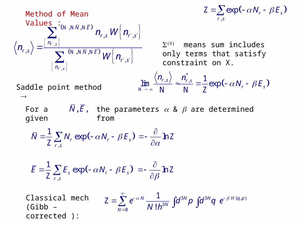
Method of Mean Values :

,

,

, ,

, ,

, , ,

,

r s

r s

N E

r s r sn

r s N E

r sn

n W n

nW n

N N N

N N N(X) means sum includes only terms that satisfy constraint on X.

Saddle point method

For a given , ,N E the parameters & are determined from

ln

Z

ln

Z

,

exp r sr s

N E Z

*

, , 1lim exp

r s r sr s

n nN E

N N N Z

,

1expr r s

r s

N N N E Z

,

1exps r s

r s

E E N E Z

Classical mech (Gibb –corrected ):

3 3 ( , )3

0

1

!N N N H q p

NN

e d p d q eN h

Z

4.3. Physical Significance of Various Statistical Quantities

The q-potential is defined as , , lnsq E Z

1 ln ln lns

s s

dq d d d EE

Z Z ZZ

,,

r s sr s

dq N d E d n d E N

lnN

Z lnE

Z

,r s

s

n N

, 1exp

r s

r s

nN E

N Z

,

exp r sr s

N E Z

,

ln 1exp r s

r ss

N EE

ZZ

dEs caused by dV.

E TS PV N

,,

r s sr s

dq N d E d n d E N

d q N E dq N d E d d N dE

,,

1r s s

r s

n d E d N dE

N

W dN dE

Q

1

kT

kT

Sq N E

k

1q N E T S

kT 1

N AkT

1G A

kT

lnPV

qkT

ZEuler’s eq.

,

exp r sr s

N E ZlnPV

qkT

Z

Fugacity /kTz e e ,

exprNs

r s

z E Z

,

ln exprNs

r s

q z E

0

ln , ,r

r

Nr

N

z Z N T V

0

ln ,r

r

r

NN

N

z Q T V

0, , 1Z T V

, ,z T VZ , ,T V Z ZVariable dependence : , ,z T VQ

Grand partition function

Note: Z is much easier to evaluate than Z,

especially for quantum statistics and/or interacting systems.

0

, ,r

r

Nr

N

z Z N T V

Grand Potential Approach

lnN

Z

lnE

Z F

Let F be the thermodynamic potential related to Z.

T

FN

, ,...F F T

lnF k T Z

kT

1

kT

FF

lnkT

Z

N N

Grand potentialParticle, heat reservoir

Suggestion from canonical ensemble :

T

F F F

T

F FT T

T T

lnE

ZF

F

kT

FT S N

2

dd dT

kT kT

T T

E F TS N U

Grand Potential See Reichl, §2.F.5.

Grand potential : lnF kT Z , ,F T V kT q

PV

d F S dT P dV N d

F U T S N

, ,F T V z

/ ,kTz e z T

,T

FP

V

F

V kT

qV

,T V

FN

/kT

T T

e

kT z

T

z

kT z

,

ln

T V

kT

Z

,

ln

T V

zz

Z

,T V

qz

z

lnU E

Z 2

,

ln

V z

kTT

Z 2

,V z

qkT

T

A N

A N F ln lnN kT z kT Z lnN

kTz

Z ln , ,kT Z N T V

Caution :

Prob 4.2

,V

FS

T

,

lnln

V

k kTT

ZZ

, , , ,

ln ln ln

V z V T V V

z

T T z T

Z Z Z

Using , , ,y z x y

f f f zf x y f x z x y

x x z x

we have

,

ln lnln

z V

zS k kT N

T T

ZZ

1

,,

lnexprN

r sr sT V

zN z E

z

ZZ

,

exprNs

r s

z E Z

N

z 2

,V

z z

T kT

lnz z

T

,

lnz V

qk q kT Nk z

T

4.4. Examples

Classical Ideal Gas :

1 ,, , ,

!

N

N

Q T VZ N T V Q T V

N

N ! = Correction for Indistinguishableness

1 ,Q T V V f TFreely moving particles

0

, , , ,r

r

Nr

N

z T V z Z N T V

Z

lnq zV f T Z

0 !

r

r

r

N

N

N r

V fz

N

exp zV f T

lnF kT kT zV f T Z

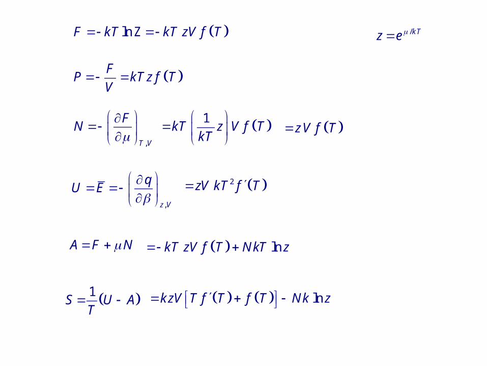
lnF kT kT zV f T Z

FP kT z f T

V

,T V

FN

1

kT z V f TkT

z V f T

/kTz e

,z V

qU E

2zV kT f T

A F N lnkT zV f T NkT z

1S U A

T lnk zV T f T f T Nk z

PV kT N

2 f TU NkT

f T

,

V

V N

UC

T

2

2 222

f T f T f TNk T T T

f T f T f T

FP kT z f T

V N zV f T 2U zV kT f T

nf T T

U NkT n

22 1VC Nk n n n n Nkn

1kT N UP

V n V

n = 3/2 : nonrelativistic gas.

n = 3 : relativistic gas.

Find A & S as functions of (T,V,N) yourself.

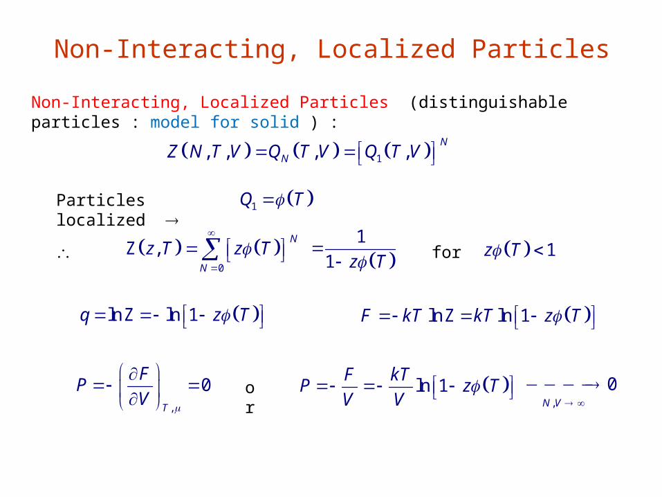
Non-Interacting, Localized Particles

Non-Interacting, Localized Particles (distinguishable particles : model for solid ) :

1, , , ,N

NZ N T V Q T V Q T V

Particles localized 1Q T

0

,N

N

z T z T

Z 1

1 z T 1z T for

ln ln 1q z T Z ln ln 1F kT kT z T Z

,

0T

FP

V

ln 1F kT

P z TV V

,

0N V

or

ln 1F kT z T

T

FN

/ln 1 kTkT e T

T

z F

kT z

1

z T

z T

z

qU E

2

1

z TkT

z T

A F N

1S U A

T

2

z

qkT

T

ln 1q z T

ln 1 lnkT z T NkT z

2 TNkT

T

ln 1 ln

1

NkT N NkT

N T

1

Nz T

N

ln 1 ln

1

z TkT k z T Nk z

z T

lnln

A NkT T O

N N

ln

lnTS N

T T ONk T N

See §3.8 11

2sinh2

T

Quantum 1-D oscillators:

kTT

Classical limit : 0

kT

Consider a substance in vapor-solid phase equilibrium inside a closed vessel .

g sz zg sT T g s i.e.,

g sV V V

g

gg

Nz

V f T

1s

ss

Nz

N T

1

T

Phase equilibrium

g

g

N f T

V T

g

g

N f T

V T

For ideal gas vapor :g

gg

NP kT

V

f T

kTT

For a monatomic gas :

nf T T

3

2U NkT

U nNkTIf

3/2f T T

From §3.5 13

1Qf T

V

Einstein model : solid ~ 3-D oscillators of same 3

1

12sinh

2

T

22

mkT

3

3/2 /3

1 12 2sinh

2kT

gP kT mkT eh

g

f TP kT

T 3

1f T

3

1

12sinh

2

T

( e / kT added by hand to account for the difference

between binding energies of the solid & gas phases. )

At phase equilibrium:

/

g

kT

N f T

V T e

Solid phase appears :

/kT

f TN

V T e

cT T

Pure vapor :

/ c

g ckT

c

N f TN

V V T e

s gN N N

Tc = characteristic TgN N

or

/ /c

ckT kT

c

f T f T

T e T e

Since f / e / kT increases with T , this means

/1 ( )s kTQ T e

Mathematica

4.5. Density & Energy Fluctuations in the Grand Canonical Ensemble:

Correspondence with Other Ensembles

,

1r sN E

rr s

N N e Z ,

r sN E

r s

e Zwith

2

, sE

NN

see §3.6

,T V

N

s sE E V

kT

,T V

NkT

,

ln 2s

nn n

n

E

N n

ZIn general

Particle density : N

nV

2 2

2 2

n N

n N

2

,T V

kT N

N

2,T V

NN kT

Particle volume : V

vN

2

22

,

/

/ T V

n V vkT

n V v

T

kT v

V

Euler’ s equation : U T S PV N

1st law : dU T d S P dV d N 0S dT V d P N d

d s dT v d P

22

1

T

n kT v

n V v P

Td vd P

T

kT

V T = isothermal

compressibility

22 T

n kT

n V

T

kT

vN

Relative root mean square of n

2

TnO

n N

~ 0 in the thermodynamic limit for finite T

At phase transition : / dT cT N , = critical exponents

d = dimension of system

Experiment on liquid-vapor transition : 0.63T cT N

2

2 nn N

n

root mean square of n0.63

0.82NN N

N

critical opalescence

Grand canonical canonical ensemble

Energy Fluctuations

2

, sE

EE

2

,z V

UkT

T

/

,

r s

kT

s s

N E

r s

z e e

U E

E E V

e

Z

, , , ,z V N V z V T V

U U N U

T T T N

,z z N T

Caution : N = N( P,T )

,

lnV

N

Z,

lnV

U

Z

2

, ,

lnV V V

N U

Z

2

, ,

1

z V V

N N

T kT

2

,

1

T V

U

kT

,

1

T V

U

T

2 2

,z V

UE kT

T

, , , ,z V N V z V T V

U U N U

T T T N

, ,

1

z V T V

N U

T T

, ,

1V

T V T V

U UC

T N

2 2

, ,

V

T V T V

U UE kT C kT

N

2, ,V V

N NN kT

§3.6 :

2 2V

can

E kT C

, , ,T V T V T V

U U N

N

2

,T V

NU

N kT

2

2 2 2

,grand can T V

UE E N

N

4.6. Thermodynamic Phase Diagrams

Phase diagram: Thermodynamic functions are analytic within a single phase,

non-analytic on phase boundaries.

Tt = 83.8 KPt = 68.9 kPa

TC = 150.7 KPC = 4.86 MPa

supercritical fluid

A = Triple pointC = Critical point

Ar

Co-existence lines :

S-LL-VS-V

Solid

Liquid

Vapor

ArTriple pointTt = 83.8 KPt = 68.9 kPa

Critical pointTC = 150.7 KPC = 4.86 MPa

supercritical fluid

Co-existence lines :

S-LL-VS-V

supercritical fluid

Co-existence lines :

S-LL-VS-V

supercritical fluid

Solid

Liquid

Vapor

4He

4He (BE stat) :Critical pointTC = 5.19 KPC = 227 kPa

T = 2.18 KPS = 2.5MPa

Superfluid characteristics (BEC) :

Viscosity = 0.

Quantized flow.

Propagating heat modes.

Macroscopic quantum coherence.

3He (FD stat) :Critical pointTC = 3.35 KPC = 227 kPa

PS = 30MPa

Superfluid below 10 mKdue to BCS p-wave pairing.

4.7. Phase Equilibrium & the Clausius-Clapeyron Equation

, ,G N P T U T S PV Gibbs free energy A PV N

= ( P,T ) = chemical potential

A BN N N

Consider vessel containing N molecules at constant T & P.

Let there be 2 phases initially: vapor (A) & liquid (B).

A BG G G A A B BN N

For a given T & P :, ,

A BA B

A BT P T P

G GdG dN dN

N N

A A B BdG dN dN

dG d N V dP S dT

A B Ad N

At equilibrium, G is a minimum 0dG for spontaneous changes

See Reichl §2.F

A B

0A B AdG d N T, P fixed for spontaneous changes

At coexistence so that NA can assume any value between 0 & N.

Coexistence curve in P-T plane is given by P P T

where , ,A BP T T P T T

Actual NA assumed is determined by U ( via latent heat of vaporization ).

A A A

P T

d P

dT T P T

B B B

P T

d P

dT T P T

d v d P s dT P

Ss

T N

T

Vv

P N

A A B B

P Ps v s v

T T

A A B B

P Ps v s v

T T

B A

B A

P s s

T v v

s

v

L

T v

Clausius-Clapeyron eq.( for 1st order transitions )

L T s Latent heat per particle.

Prob. 4.11, 4.14-6.

At triple pointA B C

Slopes ,AB AB

AB

P s

T v

,BC BC

BC

P s

T v

,CA CA

CA

P s

T v

are related

since 0AB BC CA B A C B A Cs s s s s s s s s

0AB BC CAv v v Prob. 4.17.