458 multispecies models (introduction to predator-prey dynamics) fish 458, lecture 26
TRANSCRIPT

458
Multispecies Models
(Introduction to predator-prey dynamics)
Fish 458, Lecture 26

458
Overview All of the models examined so far
ignore multispecies considerations. We can divide multispecies
considerations into biological and technological interactions.

458
Biological and Technological Interactions
Technological Interactions: linkage among species occurs because of their co-occurrence in catches.
Biological Interactions: linkage among species occurs because one eats the other or they compete for the same prey.
This lecture and the next lecture will focus on biological interactions.

458
Biological Interactions We will develop our models of biological
interactions using lumped differential equations (i.e. we are modelling the rate of change of population size / biomass).
Multi-species / eco-system models are, however, extremely complicated and we will quickly have to resort to numerical methods to make use of them.
458
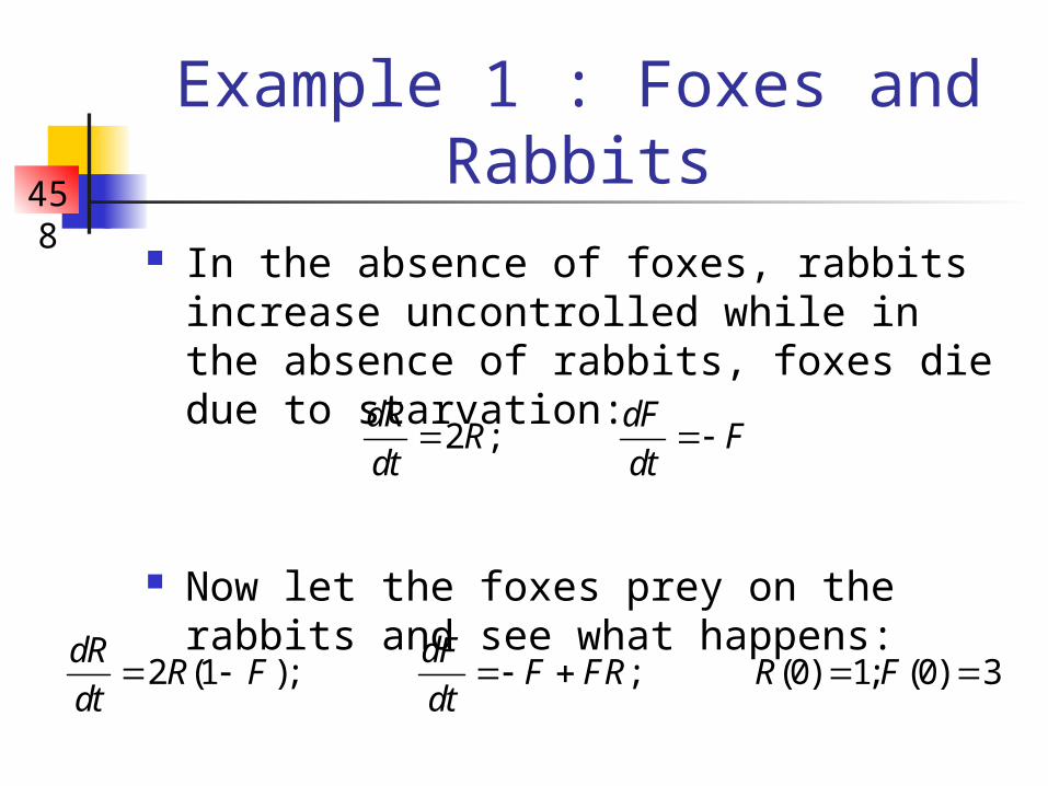
Example 1 : Foxes and Rabbits
In the absence of foxes, rabbits increase uncontrolled while in the absence of rabbits, foxes die due to starvation:
Now let the foxes prey on the rabbits and see what happens:
2 ;dR dF
R Fdt dt
2 (1 ); ; (0) 1; (0) 3dR dF
R F F FR R Fdt dt

458
Example 1 : Foxes and Rabbits
0
1
2
3
4
0 10 20 30 40 50
Time
Ab
un
da
nce
Rabbits
Foxes

458
How Did We Do That? Simple method:
Keep h very small. However, this simple approach can be very inaccurate.
I used the Runge-Kutta method – it is much more accurate (and pretty fast).
( )( ) ( ) ii i
dy ty t h y t h
dt
458
Understanding Predator-prey Dynamics
The properties of the predator-prey system can be worked out from the form of the differential equation – the phase diagram.
The population trajectories will often be strongly impacted by the initial conditions.
458
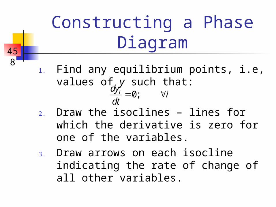
Constructing a Phase Diagram
1. Find any equilibrium points, i.e, values of y such that:
2. Draw the isoclines – lines for which the derivative is zero for one of the variables.
3. Draw arrows on each isocline indicating the rate of change of all other variables.
0;idy idt

458
Back to Foxes and Rabbits The equilibrium point is (F=1,R=1). The isoclines are defined by:
1; 1F R
0
1
2
3
4
5
0 1 2 3 4 5
Foxes
Ra
bb
its Isoclines

458
Adding in Rates of Change
0
1
2
3
4
5
0 1 2 3 4 5
Foxes
Ra
bb
its
Rabbits unchanging Foxes increasing

458
But Rabbit Populations don’t Grow Forever!
We will extend the model by allowing for some density-dependence in the growth rate for the rabbit population, i.e.:
2 (1 / 5) 2 ;
(0) 1; (0) 3
dR dFR R RF F FR
dt dtR F

458
This stablizes the population
0
1
2
3
4
0 10 20 30 40 50
Time
Ab
un
da
nce
Rabbits
Foxes

458
Computing the Phase Diagram We proceed as before
Compute the equilibrium point (R=1;F=0.8).
Compute the iscolines:
1 /5; 1F R R

458
The Phase Diagram-I
0
1
2
3
4
5
0 1 2 3 4 5
Foxes
Ra
bb
its
The point (R=1;F=0.8) is a stable equilibrium
t=0

458
The Phase Diagram-II
0
0.5
1
1.5
2
2.5
3
3.5
0 0.5 1 1.5 2 2.5 3
Rabbits
Fo
xes

458
Feeding Functional Relationships - I
The current model assumes that the amount consumed per capita is related linearly to the amount of the prey.
This may be realistic at low prey population size but there must be predator saturation.
We model this effect using feeding functional relationships

458
Feeding Functional Relationships - II
0
25
50
75
100
0 25 50 75 100
Prey Population Size
Co
sum
ptio
n r
ate
Type 1
Type 2
Type 3

458
Feeding Functional Relationships - III
2 (1 / 5) 2 ;0.6 0.6 0.6 0.6
(0) 1; (0) 3
dR R dF RR R F F F
dt R dt RR F
0
1
2
3
4
0 10 20 30 40 50
Time
Ab
un
da
nce
Rabbits
Foxes

458
Multispecies Models Advantages:
Predator-prey dynamics are clearly realistic!
Managers are often interested in “ecosystem considerations”.

458
Multispecies Models Disadvantages:
It is very difficult to select functional forms / the number of species.
The number of parameters in a multispecies model can be enormous (‘000s).
The results of multispecies models are often sensitive to their specifications.
The methods required to conduct the numerical integrations can be complicated and, if not done correctly, numerical integration impacts the results markedly.

458
Readings Press et al. (1988), Chapter 16. Starfield and Bleloch, Chapter 6.