4.3 ultrasonic computed tomography - purdue …malcolm/pct/cti_ch04.3.pdftransmittin transducer (4...

reconstruction in this study) to record total transmission loss for each ray in each projection. Then, in the positron emission study, the data for each ray can simply be attenuation compensated when corrected (by division) by this transmission loss factor. This method of attenuation compensation has been used in the PETT and other [Bro78] positron emission scanners.

There are other approaches to attenuation compensation in positron CT [Cho77]. For example, at 511-keV photon energy, a human head may be modeled as possessing constant attenuation (which is approximately equal to that of water). If in a head study the head is surrounded by a water bath, the attenuation factor given by (34) may now be easily calculated from the shape of the water bath [Eri76].

4.3 Ultrasonic Computed Tomography

When diffraction effects can be ignored, ultrasound CT is very similar to x-ray tomography. In both cases a transmitter illuminates the object and a line integral of the attenuation can be estimated by measuring the energy on the far side of the object. Ultrasound differs from x-rays because the propagation speed is much lower and thus it is possible to measure the exact pressure of the wave as a function of time. From the pressure waveform it is possible, for example, to measure not only the attenuation of the pressure field but also the delay in the signal induced by the object. From these two measurements it is possible to estimate the attenuation coefficient and the refractive index of the object. The first such tomograms were made by Greenleaf et al. [Gre74], [Gre75], followed by Carson et al. [Car76], Jackowatz and Kak [Jak76], and Glover and Sharp [Glo77].

Before we discuss ultrasonic tomography any further it should be borne in mind that the conventional method of using pulse-echo ultrasound to form images is also tomographic-in the sense that it is cross-sectional. In other words, in a conventional pulse-echo B-scan image (see Chapter 8), tissue structures aren’t superimposed upon each other. One may, therefore, ask: Why computerized ultrasonic tomography? The answer lies in the fact that with pulse-echo systems we can only see tissue interfaces, although, on account of scattering, there are some returns from within the bulk of the tissue. [Work is now progressing on methods of correlating (quantitatively) these scattered returns with the local properties of tissue [Fla83], [Kuc84]. This correlation is made difficult by the fact that the scattered returns are modified every time they pass through an interface; hence the interest in computed ultrasonic tomography as an alternative strategy for quantitative imaging with sound.]

From the discussion in a previous chapter on algorithms, it is clear that in computerized tomography it is essential to know the path that a ray traverses from the source to the detector. In x-ray and emission tomography these paths are straight lines (within limits of the detector collimators), but this isn’t always the case for ultrasound tomography. When an ultrasonic beam

MEASUREMENT OF PROJECTION DATA 147

propagates through tissue, it undergoes a deflection at every interface between tissues of different refractive indices. Carson et al. [Car771 have discussed some of the distortions introduced in a CT image by hard tissues such as bone. (For a computer simulation study of these distortions, see [Far78].) It has been suggested [Joh75] that perhaps we could correct for refraction by using the following iterative scheme: we could first reconstruct a refractive index tomogram ignoring refraction; rays could then be digitally traced through this tomogram indicating the propagation paths; these curved paths could then be used for a subsequent reconstruction, and the process repeated. Another possible approach is to use inverse scattering solutions to the problem [Iwa75], [Mue80]. Both of these approaches will be discussed in later chapters. The problem of tomographic imaging of hard tissues with ultrasound remains unsolved.

In this section we will assume that we are only dealing with soft-tissue structures. (The refraction effects are much smaller now and can generally be ignored.) An important application of this case is ultrasonic tumor detection in the female breast [Car78b], [Gre78], [Gregl], [Sch84].

Our review here will only deal with transmission ultrasound. Recently it has been shown theoretically that it is also possible to achieve (computed) tomographic imaging with reflected ultrasound [Nor79a], [Nor79b]. Clinical verification of this new technique has yet to be carried out. (See Chapter 8 for more information.)

4.3.1 Fundamental Considerations

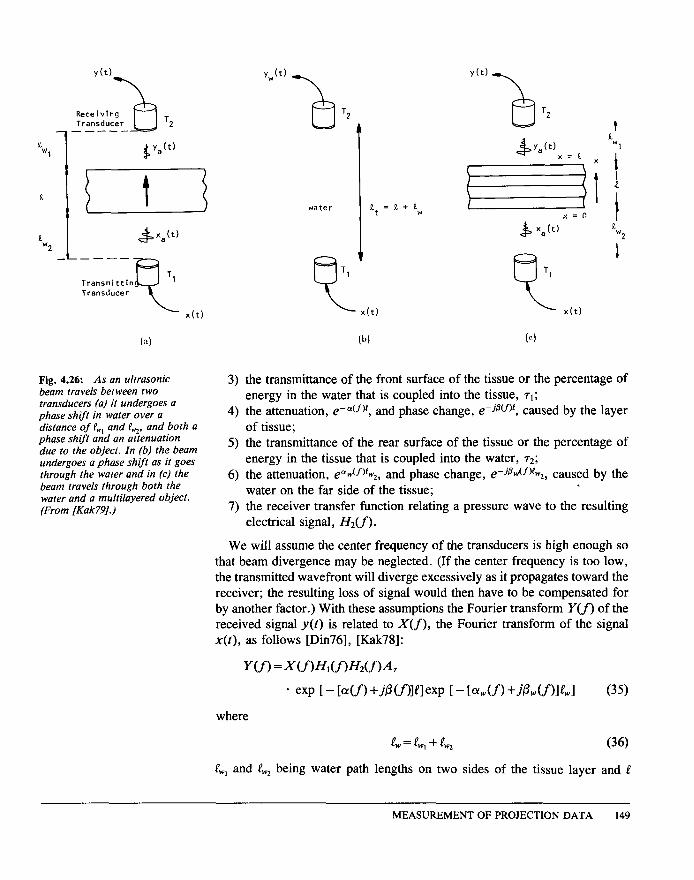
Like the x-ray case, first consider ultrasonic waves propagating from a transmitting transducer through a single layer of tissue and measured by a receiver on the far side of the tissue, as diagrammed in Fig. 4.26(a). Because ultrasonic waves in the range 1 to 10 MHz are highly attenuated by air, the tissue layer is immersed in water or another fluid. Water serves to couple the energy of the transducer into the object and provides a good refractive index match with the tissue. Ignoring the effects of refraction, here we will model the received waveform by considering only the direct path (or ray) between the two transducers.

If an electrical signal, x(t), is applied to the transmitting transducer as shown in Fig. 4.26(a), a number of effects can be identified that determine the electrical signal produced by the receiving transducer. We can write an expression for the received signal, y(t), by considering each of these effects in the frequency domain. Thus the Fourier transform of the received signal, Y(f), is given by a simple multiplication of the following factors:

1) the transmitter transfer function relating the electrical signal to the resulting pressure wave, N,(f);

2) the attenuation, e- olw(f)Pw,, and phase change, e-jpw(f)pw,, caused by the water on the near side of the tissue;

148 COMPUTERIZED TOMOGRAPHIC IMAGING

Transmittin Transducer

(4

Fig. 4.26: As an ultrasonic beam travels between two transducers (a) it undergoes a phase shift in water over a distance of PW, and t&, and both a phase shift and an attenuation due to the object. In (b) the beam undergoes a phase shift as it goes through the water and in (c) the beam travels through both the water and a multi layered object. (From [Kak79].)

v,(t)

a T2

water

6 Tl B T1 L x(t) L x(t)

(b) (cl

3) the transmittance of the front surface of the tissue or the percentage of energy in the water that is coupled into the tissue, 71;

4) the attenuation, e-OL(fjP, and phase change, e-ismr, caused by the layer of tissue;

5) the transmittance of the rear surface of the tissue or the percentage of energy in the tissue that is coupled into the water, 72;

6) the attenuation, e+Jf)tw,, and phase change, e-jfldf)C,, caused by the water on the far side of the tissue; .

7) the receiver transfer function relating a pressure wave to the resulting electrical signal, Hz(f).

We will assume the center frequency of the transducers is high enough so that beam divergence may be neglected. (If the center frequency is too low, the transmitted wavefront will diverge excessively as it propagates toward the receiver; the resulting loss of signal would then have to be compensated for by another factor.) W ith these assumptions the Fourier transform Y(f) of the received signal y(t) is related to X(f), the Fourier transform of the signal x(t), as follows [Din76], [Kak78]:

Y(f) =~m~df)~2m~7

* exp [ - b(f) +AWllWxp [ - [GU) +.A(.f)l~wl (35)

where

c = f&v, + &* (36)

C, and e,, being water path lengths on two sides of the tissue layer and 0


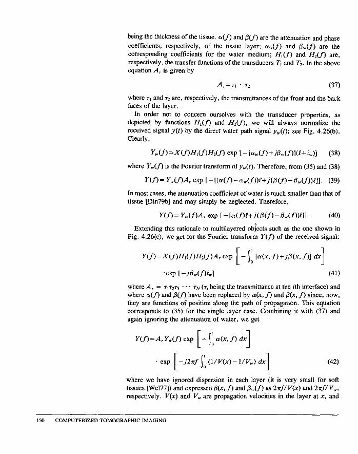
being the thickness of the tissue. a(f) and /3(f) are the attenuation and phase coefficients, respectively, of the tissue layer; a,(f) and P,,(f) are the corresponding coefficients for the water medium; Hi(j) and Hz(f) are, respectively, the transfer functions of the transducers T, and T2. In the above equation A, is given by

A~=T, * r2 (37)

where 7l and 72 are, respectively, the transmittances of the front and the back faces of the layer.

In order not to concern ourselves with the transducer properties, as depicted by functions H,(f) and Hz(f), we will always normalize the received signal y(t) by the direct water path signal y,(t); see Fig. 4.26(b). Clearly,

Y&f) =~(f)~d.f)~2(f) exp t - l%U) +AMf)l(f+ &)I (38)

where Y,(f) is the Fourier transform of y,(t). Therefore, from (35) and (38)

Y(f) = Ydf)A exp [ - [G-G) - %v(f))~+m(f) - Pwm)~ll. (39)

In most cases, the attenuation coefficient of water is much smaller than that of tissue [Din79b] and may simply be neglected. Therefore,

Y(f) = Y&%4, exp [ - M fY+.WW - ,&Lf))~ll. (40)

Extending this rationale to multilayered objects such as the one shown in Fig. 4.26(c), we get for the Fourier transform Y(f) of the received signal:

-exp [ -ALUYwl (41)

where A, = ~17273 * * * rN (7; being the transmittance at the ith interface) and where o(f) and /3(f) have been replaced by CY(X, f) and p(x, f) since, now, they are functions of position along the path of propagation. This equation corresponds to (35) for the single layer case. Combining it with (37) and again ignoring the attenuation of water, we get

* exp [ s

-j2rf ’ (l/V(x)- l/V,) dx 1 (42) 0

where we have ignored dispersion in each layer (it is very small for soft tissues [We177]) and expressed 0(x, f) and P,(f) as 2?rf/ V(x) and 2?rf/ V,, respectively. V(x) and V, are propagation velocities in the layer at x, and


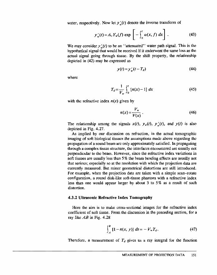
water, respectively. Now let y;(t) denote the inverse transform of

We may consider y;(t) to be an “attenuated” water path signal. This is the hypothetical signal that would be received if it underwent the same loss as the actual signal going through tissue. By the shift property, the relationship depicted in (42) may be expressed as

where

u(O=y:(t- Ted (44)

Ti=+ ip [n(x)-- 11 dx w 0

with the refractive index n(x) given by

VW n(x)=-. VW

(46)

The relationship among the signals x(t), y,,,(t), y:(t), and y(t) is also depicted in Fig. 4.27.

As implied by our discussion on refraction, in the actual tomographic imaging of soft biological tissues the assumptions made above regarding the propagation of a sound beam are only approximately satisfied. In propagating through a complex tissue structure, the interfaces encountered are usually not perpendicular to the beam. However, since the refractive index variations in soft tissues are usually less than 5 % the beam bending effects are usually not that serious; especially so at the resolution with which the projection data are currently measured. But minor geometrical distortions are still introduced. For example, when the projection data are taken with a simple scan-rotate configuration, a round disk-like soft-tissue phantom with a refractive index less than one would appear larger by about 3 to 5% as a result of such distortion.

4.3.2 Ultrasonic Refractive Index Tomography

Here the aim is to make cross-sectional images for the refractive index coefficient of soft tissue. From the discussion in the preceding section, for a ray like AB in Fig. 4.28

s ’ [I-n(x,y)] ds= -V,T,. A

Therefore, a measurement of T, gives us a ray integral for the function


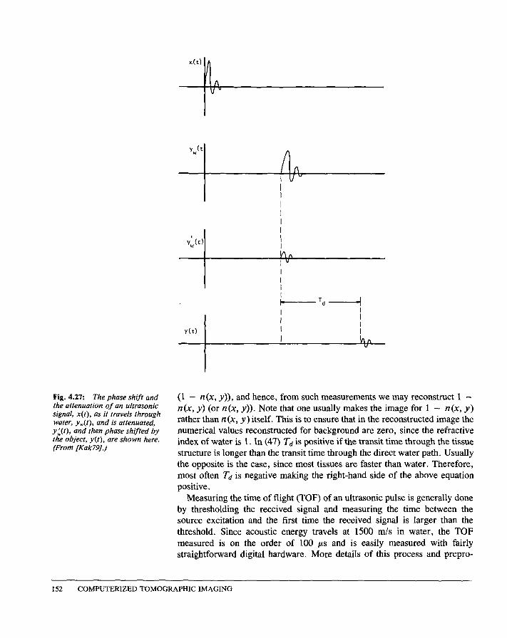
Fig. 4.27: The phase shift and the attenuation of an ultrasonic signal, x(t), as it travels through water, yW(t), and is attenuated, y;(t), and then phase shifted by the object, y(t), are shown here. (From [Kak79].)

(1 - n(x, y)), and hence, from such measurements we may reconstruct 1 - n(x, y) (or n(x, y)). Note that one usually makes the image for 1 - n(x, y) rather than n(x, y ) itself. This is to ensure that in the reconstructed image the numerical values reconstructed for background are zero, since the refractive index of water is 1. In (47) Td is positive if the transit time through the tissue structure is longer than the transit time through the direct water path. Usually the opposite is the case, since most tissues are faster than water. Therefore, most often Td is negative making the right-hand side of the above equation positive.

Measuring the time of flight (TOF) of an ultrasonic pulse is generally done by thresholding the received signal and measuring the time between the source excitation and the first time the received signal is larger than the threshold. Since acoustic energy travels at 1500 m/s in water, the TOF measured is on the order of 100 ps and is easily measured with fairly straightforward digital hardware. More details of this process and prepro-

1.52 COMPUTERIZED TOMOGRAPHIC IMAGING

y(t)

r

6 T2 ,A ‘1 !’

A

x(t)

Fig. 4.28: In ul trasound refractive index tomography the time it takes for an ul trasound pulse to travel between points A and B is measured. (From [Kak79].)

cessing algorithms that can be used to clean up the projection data are described in [Cra82].

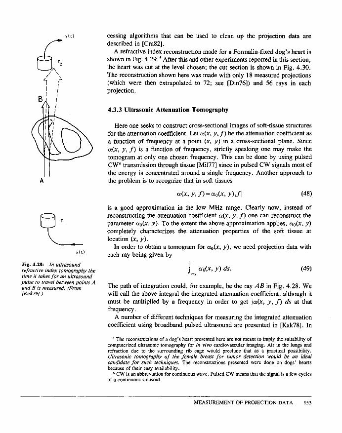
A refractive index reconstruction made for a Formalin-fixed dog’s heart is shown in Fig. 4.29. 5 After this and other experiments reported in this section, the heart was cut at the level chosen; the cut section is shown in Fig. 4.30. The reconstruction shown here was made with only 18 measured projections (which were then extrapolated to 72; see [Din76]) and 56 rays in each projection.

4.3.3 Ultrasonic Attenuation Tomography

Here one seeks to construct cross-sectional images of soft-tissue structures for the attenuation coefficient. Let CY(X, y, f) be the attenuation coefficient as a function of frequency at a point (x, y) in a cross-sectional plane. Since o(x, y, f) is a function of frequency, strictly speaking one may make the tomogram at only one chosen frequency. This can be done by using pulsed CW6 transmission through tissue [Mi177] since in pulsed CW signals most of the energy is concentrated around a single frequency. Another approach to the problem is to recognize that in soft tissues

4x9 Y9 f) = ~o(X9 Y)lfl (48).

is a good approximation in the low MHz range. Clearly now, instead of reconstructing the attenuation coefficient a(x, y, S) one can reconstruct the parameter oo(x, y). To the extent the above approximation applies, ao(x, y) completely characterizes the attenuation properties of the soft tissue at location (x, y).

In order to obtain a tomogram for (YO(X, y), we need projection data with each ray being given by

s ~o(X, Y) ds. (49) ray

The path of integration could, for example, be the ray AB in Fig. 4.28. We will call the above integral the integrated attenuation coefficient, although it must be multiplied by a frequency in order to get Ja(x, y, f) ds at that frequency.

A number of different techniques for measuring the integrated attenuation coefficient using broadband pulsed ultrasound are presented in [Kak78]. In

5 The reconstructions of a dog’s heart presented here are not meant to imply the suitability of computerized ultrasonic tomography for in vivo cardiovascular imaging. Air in the lungs and refraction due to the surrounding rib cage would preclude that as a practical possibility. Ultrasonic tomography of the female breast for tumor detection would be an ideal candidate for such techniques. The reconstructions presented were done on dogs’ hearts because of their easy availability.

6 C W is an abbreviation for continuous wave. Pulsed C W means that the signal is a few cycles of a continuous sinusoid.


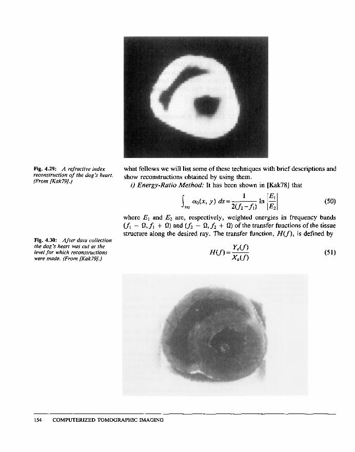
Fig. 4.29: A refractive index what follows we will list some of these techniques with brief descriptions and reconstntction of the dog

’

s

heart. (From [Kak79].)

show reconstructions obtained by using them. i) Energy-Ratio Method: It has been shown in [Kak78] that

s

1 aok Y) ds=

=aY w2 -fl)

Fig. 4.30: After data collection the dog

’

s

heart was cut at the level for which reconstructions were made. (From fKak79J.)

where El and E2 are, respectively, weighted energies in frequency bands (Jr - Q,.f, + 0) and (f2 - Q, f2 + Q) of the transfer functions of the tissue structure along the desired ray. The transfer function, H(f), is defined by

y&f 1 H(f) = - (51)

x7(f)


where Y,,(f) and X,(f) are Fourier transforms of the signals v,(t) and x,(t), respectively (Fig. 4.26(c)). One can show that in terms of the experimentally measured signals y(t) and v,,(t) [Din79b]:

(52)

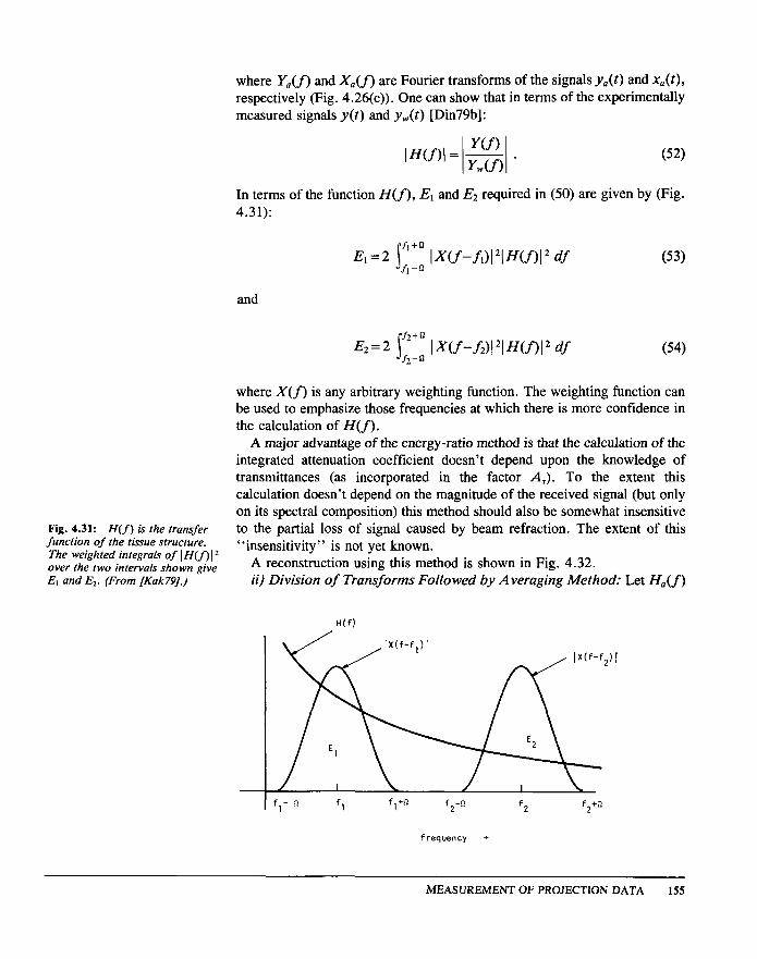
In terms of the function H(f), El and Ez required in (50) are given by (Fig. 4.31):

E,=2 1;;: IX(f-fJ121H(f)12 df (53) 1

and

E2=2 j;;; I~W-f2)121Wf)12 df 2

(54)

where X(f) is any arbitrary weighting function. The weighting function can be used to emphasize those frequencies at which there is more confidence in the calculation of H(f).

A major advantage of the energy-ratio method is that the calculation of the integrated attenuation coefficient doesn’t depend upon the knowledge of transmittances (as incorporated in the factor A,). To the extent this calculation doesn’t depend on the magnitude of the received signal (but only on its spectral composition) this method should also be somewhat insensitive

Fig. 4.31: H(J) is the transfer to the partial loss of signal caused by beam refraction. The extent of this function of the tissue structure. The weighted integrals of IH(f

“insensitivity” is not yet known. over the two intervals shown give A reconstruction using this method is shown in Fig. 4.32. El and E2. (From [Kak79].) ii) Division of Transforms Followed by Averaging Method: Let H,,(f)

H(f)

frequency -


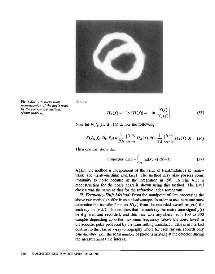
Fig. 4.32: An attenuation denote reconstruction of the dog

’

s

heart by the energy-ratio method. (From [Kak79].)

Y(f) HA(f)= -In IH(f -In - .

I I Y,(f) (55)

Now let F(fi, f2, Q,, Q2) denote the following:

F(h,fz, Ql, a,,=$ j;;: HA(f) df-& J;;l

’

HA(f) df. (56) 2 2 1 1

Then one can show that

projection data = s a,,(~, y) ds = F. (57) ray

Again, the method is independent of the value of transmittances at tissue- tissue and tissue-medium interfaces. The method may also possess some immunity to noise because of the integration in (56). In Fig. 4.33 a reconstruction for the dog

’

s

heart is shown using this method. The level chosen was the same as that for the refractive index tomogram.

iii) Frequency-Shift Method: From the standpoint of data processing the above two methods suffer from a disadvantage. In order to use them one must determine the transfer function H(f) from the recorded waveform y(t) for each ray and y,,,(t). This requires that for each ray the entire time signal y(t) be digitized and recorded, and this may take anywhere from 100 to 300 samples depending upon the maximum frequency (above the noise level) in the acoustic pulse produced by the transmitting transducer. This is in marked contrast to the case of x-ray tomography where for each ray one records only one number, i.e., the total number of photons arriving at the detector during the measurement time interval.

156 COMPUTERIZED TOMOCXAPHIC IMAGING

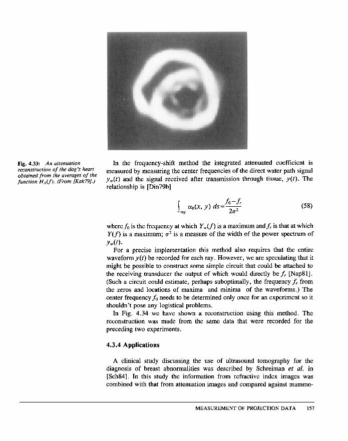
Fig. 4.33: An attenuation In the frequency-shift method the integrated attenuated coefficient is reconstruction of the dog

’

s

heart obtained from the averages of the

measured by measuring the center frequencies of the direct water path signal function H..,(f). (From [Kak791.) y,,,(t) and the signal received after transmission through tissue, y(t). The

relationship is [Din79b]

s ray ao(x, y) ds=fg (58)

where f. is the frequency at which Y,(f) is a maximum and fr is that at which Y(f) is a maximum; u2 is a measure of the width of the power spectrum of

YWW. For a precise implementation this method also requires that the entire

waveform y(t) be recorded for each ray. However, we are speculating that it might be possible to construct some simple circuit that could be attached to the receiving transducer the output of which would directly be fr [Nap8 11. (Such a circuit could estimate, perhaps suboptimally, the frequency fr from the zeros and locations of maxima and minima of the waveforms.) The center frequency f. needs to be determined only once for an experiment so it shouldn

’

t

pose any logistical problems. In Fig. 4.34 we have shown a reconstruction using this method. The

reconstruction was made from the same data that were recorded for the preceding two experiments.

4.3.4 Applications

A clinical study discussing the use of ultrasound tomography for the diagnosis of breast abnormalities was described by Schreiman et al. in [Sch84]. In this study the information from refractive index images was combined with that from attenuation images and compared against mammo-


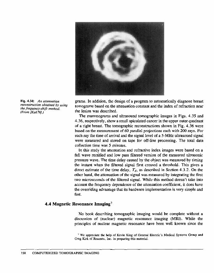
Fig. 4.34: An attenuation reconstruction obtained by using the frequency-shift method. (From [Kak79J.)

grams. In addition, the design of a program to automatically diagnose breast tomograms based on the attenuation constant and the index of refraction near the lesion was described.

The mammograms and ultrasound tomographic images in Figs. 4.35 and 4.36, respectively, show a small spiculated cancer in the upper outer quadrant of a right breast. The tomographic reconstructions shown in Fig. 4.36 were based on the measurement of 60 parallel projections each with 200 rays. For each ray the time of arrival and the signal level of a ~-MHZ ultrasound signal were measured and stored on tape for off-line processing. The total data collection time was 5 minutes.

In this study the attenuation and refractive index images were based on a full wave rectified and low pass filtered version of the measured ultrasonic pressure wave. The time delay caused by the object was measured by timing the instant when the filtered signal first crossed a threshold. This gives a direct estimate of the time delay, Td, as described in Section 4.3.2. On the other hand, the attenuation of the signal was measured by integrating the first two microseconds of the filtered signal. While this method doesn

’

t

take into account the frequency dependence of the attenuation coefficient, it does have the overriding advantage that its hardware implementation is very simple and fast.

4.4 Magnetic Resonance Imaging

’

No book describing tomographic imaging would be complete without a discussion of (nuclear) magnetic resonance imaging (MRI). While the principles of nuclear magnetic resonance have been well known since the

’ We appreciate the help of Kevin King of General Electric

’

s

Medical Systems Group and Greg Kirk of Resonex, Inc. in preparing this material.


4.3 ultrasonic computed tomography - purdue …malcolm/pct/cti_ch04.3.pdftransmittin transducer (4...

Documents