42-1Copyright 2010 McGraw-Hill Australia Pty Ltd PowerPoint slides to accompany Biology: An Australian focus 4e by Knox, Ladiges, Evans and SaintSlides prepared by Karen Burke da Silva, Flinders University

Chapter 42: Population ecology

42-2Copyright 2010 McGraw-Hill Australia Pty Ltd PowerPoint slides to accompany Biology: An Australian focus 4e by Knox, Ladiges, Evans and SaintSlides prepared by Karen Burke da Silva, Flinders University

What is a population? • ‘A number of organisms of the same species in a

defined geographical area’• Properties of populations include:

– number of individuals– area they occupy– age structure– sex ratio

• Different processes (e.g. fire, herbivory) may be important at different times in the life cycle (e.g. fire destroys adult golden wattle trees, but the seeds often need fire to germinate)

42-3Copyright 2010 McGraw-Hill Australia Pty Ltd PowerPoint slides to accompany Biology: An Australian focus 4e by Knox, Ladiges, Evans and SaintSlides prepared by Karen Burke da Silva, Flinders University

Distribution and abundance of populations• Biotic and abiotic factors control populations• A direct factor (e.g. water availability) may be

controlled by several indirect factors (e.g. temperature, rainfall; see Fig. 42.2a)

• The probability of occurrence of a species plotted against an environmental gradient defines the realised distribution, or niche, of the species in environmental space

• The realised niche is a subset of the fundamental niche

• Space and time also cause population fluctuations

42-4Copyright 2010 McGraw-Hill Australia Pty Ltd PowerPoint slides to accompany Biology: An Australian focus 4e by Knox, Ladiges, Evans and SaintSlides prepared by Karen Burke da Silva, Flinders University

Fig. 42.2a: Probability of occurrence of different eucalypts

42-5Copyright 2010 McGraw-Hill Australia Pty Ltd PowerPoint slides to accompany Biology: An Australian focus 4e by Knox, Ladiges, Evans and SaintSlides prepared by Karen Burke da Silva, Flinders University

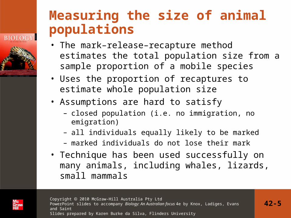
Measuring the size of animal populations• The mark–release–recapture method estimates

the total population size from a sample proportion of a mobile species

• Uses the proportion of recaptures to estimate whole population size

• Assumptions are hard to satisfy– closed population (i.e. no immigration, no emigration)– all individuals equally likely to be marked– marked individuals do not lose their mark

• Technique has been used successfully on many animals, including whales, lizards, small mammals

42-6Copyright 2010 McGraw-Hill Australia Pty Ltd PowerPoint slides to accompany Biology: An Australian focus 4e by Knox, Ladiges, Evans and SaintSlides prepared by Karen Burke da Silva, Flinders University

Density-independent population dynamics

• Population size changes are due only to birth, death, immigration and emigration

• When birth and death rates are not affected by population size, they are ‘density-independent’

• Closed populations have no immigration or emigration

42-7Copyright 2010 McGraw-Hill Australia Pty Ltd PowerPoint slides to accompany Biology: An Australian focus 4e by Knox, Ladiges, Evans and SaintSlides prepared by Karen Burke da Silva, Flinders University

Exponential population growth in discrete time• Number of females in a closed population at time

(t + 1) is N(t+1) and is related to the number at the previous time (t) by:

so

(where b and d are birth and death rates, respectively)

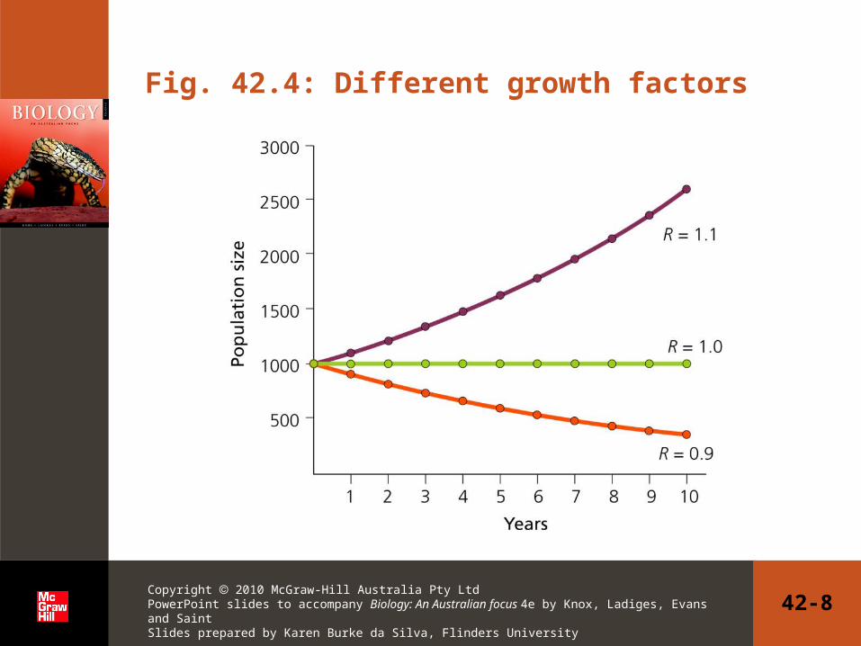
• If Rt, the growth factor each year, is constant

• Small changes in R have major effects on population size; see Fig. 42.4

)1(1 ttttt dNbNN

ttt NRN 1

0NRN tt

42-8Copyright 2010 McGraw-Hill Australia Pty Ltd PowerPoint slides to accompany Biology: An Australian focus 4e by Knox, Ladiges, Evans and SaintSlides prepared by Karen Burke da Silva, Flinders University

Fig. 42.4: Different growth factors

42-9Copyright 2010 McGraw-Hill Australia Pty Ltd PowerPoint slides to accompany Biology: An Australian focus 4e by Knox, Ladiges, Evans and SaintSlides prepared by Karen Burke da Silva, Flinders University

Environmental variability and exponential growth

• Mean exponential growth rate over several years is given by the geometric (not arithmetic) mean, called ‘R’

• To calculate R, find the nth root of the product of R values for n years

• A closed, density-independent population will either grow or reduce exponentially depending on whether R is >1 or <1 respectively

• If R = 1, the population size will remain constant

42-10Copyright 2010 McGraw-Hill Australia Pty Ltd PowerPoint slides to accompany Biology: An Australian focus 4e by Knox, Ladiges, Evans and SaintSlides prepared by Karen Burke da Silva, Flinders University

Table 42.1: Geometric mean and population size

42-11Copyright 2010 McGraw-Hill Australia Pty Ltd PowerPoint slides to accompany Biology: An Australian focus 4e by Knox, Ladiges, Evans and SaintSlides prepared by Karen Burke da Silva, Flinders University

Exponential population growth in continuous time• For organisms that breed throughout the year,

differential equations best describe population growth

• This gives the intrinsic rate of increase, denoted by a lower case ‘r’

• In the continuous time model of exponential growth, the intrinsic rate of growth r determines the fate of the population

ttt

rNNdbdt

dN )(

42-12Copyright 2010 McGraw-Hill Australia Pty Ltd PowerPoint slides to accompany Biology: An Australian focus 4e by Knox, Ladiges, Evans and SaintSlides prepared by Karen Burke da Silva, Flinders University

Range expansions• Initial expansion of a species is often exponential • The boundary often spreads at a constant rate• Rate of spread is proportional to the growth rate of

the population• This phenomenon has been observed for many

plant and animal species (e.g. mangrove Avicennia marina in New Zealand)

42-13Copyright 2010 McGraw-Hill Australia Pty Ltd PowerPoint slides to accompany Biology: An Australian focus 4e by Knox, Ladiges, Evans and SaintSlides prepared by Karen Burke da Silva, Flinders University

Fig. 42.6a: Expansion of a population of Avicennia marina

42-14Copyright 2010 McGraw-Hill Australia Pty Ltd PowerPoint slides to accompany Biology: An Australian focus 4e by Knox, Ladiges, Evans and SaintSlides prepared by Karen Burke da Silva, Flinders University

Fig. 42.6b: Avicennia estuary

Copyright © G R Roberts, Photo Library, New Zealand

42-15Copyright 2010 McGraw-Hill Australia Pty Ltd PowerPoint slides to accompany Biology: An Australian focus 4e by Knox, Ladiges, Evans and SaintSlides prepared by Karen Burke da Silva, Flinders University

Density-dependent population dynamics

Population size does not increase indefinitely…• Negative density-dependent population growth

results from lowered birth rate or higher death rate when a resource becomes limiting

• The logistic growth curve is S-shaped because resource limitation lowers the growth rate to zero where the curve levels out to an asymptote

• The value of the asymptote on the y-axis is the carrying capacity, K, of the population

42-16Copyright 2010 McGraw-Hill Australia Pty Ltd PowerPoint slides to accompany Biology: An Australian focus 4e by Knox, Ladiges, Evans and SaintSlides prepared by Karen Burke da Silva, Flinders University

Fig. 42.7a: Antechinus stuartii

Copyright © C A Henley/AUSCAPE

42-17Copyright 2010 McGraw-Hill Australia Pty Ltd PowerPoint slides to accompany Biology: An Australian focus 4e by Knox, Ladiges, Evans and SaintSlides prepared by Karen Burke da Silva, Flinders University

Fig. 42.7b: Population size of Antechinus stuartii

42-18Copyright 2010 McGraw-Hill Australia Pty Ltd PowerPoint slides to accompany Biology: An Australian focus 4e by Knox, Ladiges, Evans and SaintSlides prepared by Karen Burke da Silva, Flinders University

Fig. 42.8: Logistic growth

42-19Copyright 2010 McGraw-Hill Australia Pty Ltd PowerPoint slides to accompany Biology: An Australian focus 4e by Knox, Ladiges, Evans and SaintSlides prepared by Karen Burke da Silva, Flinders University

Density-dependent population dynamics (cont.)• Population approaches an equilibrium state at the

carrying capacity, K• The logistic growth equation is

• As N approaches K the growth rate decreases• When N = K, the growth rate is zero• Variability in environment may override the effect

of K, as the population size may never reach it

K

NrN

dt

dN1

Question 1:

42-20Copyright 2010 McGraw-Hill Australia Pty Ltd PowerPoint slides to accompany Biology: An Australian focus 4e by Knox, Ladiges, Evans and SaintSlides prepared by Karen Burke da Silva, Flinders University

Density-dependent factors have the greatest effect on population densities when:

a) Only birth rate changes in response to density

b) Only death rate changes in response to density

c) Diseases spread in populations at all densities

d) Both birth and death rates change in response to densities

e) Population densities fluctuate very little

42-21Copyright 2010 McGraw-Hill Australia Pty Ltd PowerPoint slides to accompany Biology: An Australian focus 4e by Knox, Ladiges, Evans and SaintSlides prepared by Karen Burke da Silva, Flinders University

Is density-dependent control important or not?

• This has been a controversial topic• Plants often do show density-dependent control • In animals, environmental conditions may be

primary control; density-dependence is less likely– vertebrates maintain fairly constant population sizes– invertebrates display density-vague population

dynamics; numbers fluctuate widely and resource limitation may be rare, e.g. locusts

42-22Copyright 2010 McGraw-Hill Australia Pty Ltd PowerPoint slides to accompany Biology: An Australian focus 4e by Knox, Ladiges, Evans and SaintSlides prepared by Karen Burke da Silva, Flinders University

Space-limited populations• Sessile (fixed) organisms may compete for space

more than food, e.g. mussels, barnacles (see Fig. 42.10) and plants

• Sessile populations live in habitats that experience disturbance

• These species have good dispersal ability• Successful recruitment depends on disturbance to

provide a new space to settle• Ecological disturbance results from death of

individuals or from any space-liberating process

42-23Copyright 2010 McGraw-Hill Australia Pty Ltd PowerPoint slides to accompany Biology: An Australian focus 4e by Knox, Ladiges, Evans and SaintSlides prepared by Karen Burke da Silva, Flinders University

Fig 42.10: Competition for space

Copyright © Paddy Ryan/ANT Photo Library

42-24Copyright 2010 McGraw-Hill Australia Pty Ltd PowerPoint slides to accompany Biology: An Australian focus 4e by Knox, Ladiges, Evans and SaintSlides prepared by Karen Burke da Silva, Flinders University

Self-thinning and the law of constant yield• Plant growth patterns often show self-thinning• Seedling growth rate depends on the initial sowing

density• Plant yield (biomass x density) is constant• The ‘law of constant yield’ is used to determine

optimal sowing density for a species• With time, plants in denser plots begin to die

according to the –3/2 self-thinning rule

42-25Copyright 2010 McGraw-Hill Australia Pty Ltd PowerPoint slides to accompany Biology: An Australian focus 4e by Knox, Ladiges, Evans and SaintSlides prepared by Karen Burke da Silva, Flinders University

Fig. B42.2: The rule of constant yield

42-26Copyright 2010 McGraw-Hill Australia Pty Ltd PowerPoint slides to accompany Biology: An Australian focus 4e by Knox, Ladiges, Evans and SaintSlides prepared by Karen Burke da Silva, Flinders University

Age- and size-structured population dynamics

• Age and/or size of an individual affects its fecundity (probability of giving birth) and survival

• Treating all members of a population as identical is unrepresentative of natural population structure

• Fig. 42.11b shows how an imbalanced initial age structure generates age and number cycles

• Life tables are used to show survivorship probability at each age, but long-term studies are the key to understanding population dynamics

42-27Copyright 2010 McGraw-Hill Australia Pty Ltd PowerPoint slides to accompany Biology: An Australian focus 4e by Knox, Ladiges, Evans and SaintSlides prepared by Karen Burke da Silva, Flinders University

Fig. 42.11a: Age-structured population dynamics: balanced

Question 2:

The best way to reduce the population of an undesirable species in the long term is to:

a) Reduce the carrying capacity of the environment for the species

b) Selectively kill reproducing adults

c) Selectively kill pre-reproductive individuals

d) Attempt to kill all individuals of all ages

e) Sterilise all individuals

42-28Copyright 2010 McGraw-Hill Australia Pty Ltd PowerPoint slides to accompany Biology: An Australian focus 4e by Knox, Ladiges, Evans and SaintSlides prepared by Karen Burke da Silva, Flinders University

42-29Copyright 2010 McGraw-Hill Australia Pty Ltd PowerPoint slides to accompany Biology: An Australian focus 4e by Knox, Ladiges, Evans and SaintSlides prepared by Karen Burke da Silva, Flinders University

Fig. 42.11b: Age-structured population dynamics: imbalanced

42-30Copyright 2010 McGraw-Hill Australia Pty Ltd PowerPoint slides to accompany Biology: An Australian focus 4e by Knox, Ladiges, Evans and SaintSlides prepared by Karen Burke da Silva, Flinders University

Australia’s human population dynamics• Study of ‘human demography’• Changes in human population size are mostly due

to behavioural changes, e.g. one-child policy in China

• Economists need to know the future age structure to enable the building of more nursing homes or schools in the right places

• The current trend is toward an ageing population• Growth rate of many western countries is now

below the replacement rate, so population numbers will slowly begin to level out and then fall

42-31Copyright 2010 McGraw-Hill Australia Pty Ltd PowerPoint slides to accompany Biology: An Australian focus 4e by Knox, Ladiges, Evans and SaintSlides prepared by Karen Burke da Silva, Flinders University

Bioeconomics: managing exploited populations• This theory addresses the problem of harvesting a

population for maximum economic and social benefit

• The maximum sustainable yield (MSY) is the harvesting rate that can be maintained indefinitely

• It is prudent to harvest below the MSY rate due to uncertainty about species’ biology and stochastic (unpredictable) events

• Highly mobile species may be hard to harvest when there are only a few left, but sessile species are vulnerable to extinction

42-32Copyright 2010 McGraw-Hill Australia Pty Ltd PowerPoint slides to accompany Biology: An Australian focus 4e by Knox, Ladiges, Evans and SaintSlides prepared by Karen Burke da Silva, Flinders University

Conservation strategy for Leadbeater’s possum• Gymnobelideus leadbeateri live in mountain ash

forests where they nest in old trees• Fire and logging both reduce availability of hollows• Lindenmayer and Possingham carried out a

detailed population viability analysis of the species• Included study of habitat attributes and dynamics• The data were used to develop a population

simulation model• Enabled a suitable management plan to be

implemented to ensure survival of the possum, even with environmental and demographic uncertainty

42-33Copyright 2010 McGraw-Hill Australia Pty Ltd PowerPoint slides to accompany Biology: An Australian focus 4e by Knox, Ladiges, Evans and SaintSlides prepared by Karen Burke da Silva, Flinders University

Fig. B42.4: Leadbeater’s possum (Gymnobelideus leadbeateri)

Copyright © Fredy Mercay/ANT Photo Library

42-34Copyright 2010 McGraw-Hill Australia Pty Ltd PowerPoint slides to accompany Biology: An Australian focus 4e by Knox, Ladiges, Evans and SaintSlides prepared by Karen Burke da Silva, Flinders University

Viable population sizes for conservation

• The minimum viable population size (MVP) is different for each species, and for each set of circumstances

• All species will eventually become extinct• Chance processes may cause extinction

– genetic stochasticity, i.e. sufficient heterozygosity is needed in the population

– demographic stochasticity, i.e. the random nature of births and deaths, can wipe out a small population

– environmental stochasticity and catastrophes, e.g. fire, drought, flood can unpredictably exterminate entire populations

42-35Copyright 2010 McGraw-Hill Australia Pty Ltd PowerPoint slides to accompany Biology: An Australian focus 4e by Knox, Ladiges, Evans and SaintSlides prepared by Karen Burke da Silva, Flinders University

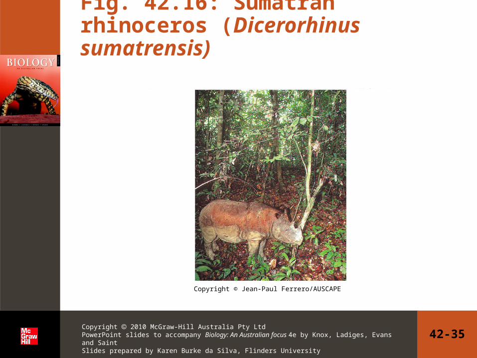
Fig. 42.16: Sumatran rhinoceros (Dicerorhinus sumatrensis)

Copyright © Jean-Paul Ferrero/AUSCAPE

Summary• Understanding the dynamics relating to distribution

and abundance of organisms is essential if natural populations are to be effectively managed

• Biotic and abiotic factors can influence the processes of population change: birth, death, immigration and emigration

• Population growth can be constrained by the availability of resources and by the space available

• The age structure of a population affects population growth

42-36Copyright 2010 McGraw-Hill Australia Pty Ltd PowerPoint slides to accompany Biology: An Australian focus 4e by Knox, Ladiges, Evans and SaintSlides prepared by Karen Burke da Silva, Flinders University