4. title and subtitle - university of texas
TRANSCRIPT

Technical Report Documentation Page 1. Report No.
FHWA/TX-04/0-4322-1 2. Government Accession No. 3. Recipient’s Catalog No.
4. Title and Subtitle DEVELOPMENT OF A NEW METHODOLOGY FOR CHARACTERIZING PAVEMENT STRUCTURAL CONDITION FOR NETWORK-LEVEL APPLICATIONS
5. Report Date October 2002 Revised August 2003
6. Performing Organization Code
7. Author(s) Zhanmin Zhang, Lance Manuel, Ivan Damnjanovic, Zheng Li 8. Performing Organization Report No.
Research Report 0-4322-1
10. Work Unit No. (TRAIS)
9. Performing Organization Name and Address Center for Transportation Research The University of Texas at Austin 3208 Red River, Suite 200 Austin, TX 78705-2650
11. Contract or Grant No. 0-4322
13. Type of Report and Period Covered Research Report (9/1/01-8/31/02)
12. Sponsoring Agency Name and Address Texas Department of Transportation Research and Technology Implementation Office P.O. Box 5080 Austin, TX 78763-5080
14. Sponsoring Agency Code
15. Supplementary Notes Project conducted in cooperation with the U.S. Department of Transportation, Federal Highway Administration, and the Texas Department of Transportation.
16. Abstract
Huge quantities of bituminous mix in the form of seal coats and HMAC thin overlays are applied by the TxDOT every year to improve ride quality and seal existing cracks, but these measures do not correct possible underlying weaknesses that will cause roughness or distress to quickly reappear. As a result, the overall pavement condition keeps deteriorating due to the structural deformation of pavement layers and the subgrade, even though surface treatments are applied periodically. The developed methodology introduces the Structural Condition Index (SCI). The SCI is based on the estimated effective Structural Number (SN), and its main purpose is to discriminate pavements that need structural reinforcement from the ones that are in sound structural condition. In addition, a contingent sampling procedure was developed to determine the minimum number of FWD tests required for each management section of pavements. The comprehensive guidelines were developed for using the SCI in the selection of the best maintenance and rehabilitation alternatives at network level. Finally, a pilot application of the SCI was carried out with several pavement rehabilitation projects to verify the validity of the developed SCI, with the intention that modifications would be made to the developed procedure if such a need is determined from the pilot application.
17. Key Words
pavement structural condition, Structural Number, pavement maintenance and rehabilitation
18. Distribution Statement No restrictions. This document is available to the public through the National Technical Information Service, Springfield, Virginia 22161.
19. Security Classif. (of report)
Unclassified 20. Security Classif. (of this page)
Unclassified 21. No. of pages
100 22. Price
Form DOT F 1700.7 (8-72) Reproduction of completed page authorized


Development of a New Methodology for Characterizing Pavement Structural Condition for Network- Level Applications
Zhanmin Zhang Lance Manuel
Ivan Damnjanovic Zheng Li
Research Report 0-4322-1
Research Project 0-4322 Develop a New Methodology for Characterizing
Pavement Structural Condition for Network-Level Application
Conducted for the Texas Department of Transportation
in cooperation with the U.S. Department of Transportation Federal Highway Administration
by the Center for Transportation Research
Bureau of Engineering Research The University of Texas at Austin
October 2002
Revised August 2003

iv

Disclaimers
The contents of this report reflect the views of the authors, who are responsible for the facts and accuracy of the data presented herein. The contents do not necessary reflect the official views or policies of the Federal Highway Administration or the Texas Department of Transportation. This report does not constitute a standard, specification, or regulation.
There was no invention or discovery conceived or first actually reduced to practice in the course of or under this contract, including any art, method, process, machine, manufacture, design or composition of matter, or any new and useful improvement thereof, or any variety of plant, which is or may be patented under the patent laws of the United States of America or any other country.
NOT INTENDED FOR CONSTRUCTION, BIDDING, OR PERMIT PURPOSES
Zhanmin Zhang, Ph.D. Research Supervisor
Acknowledgments
This project has been conducted under the guidance of, and has been directly assisted by the Project Director (PD) and the Project Monitoring Committee (PMC). We would especially like to acknowledge the following people who served on the Project Monitoring Committee.
Project Monitoring Committee
Dr. German Claros, P.E., Project Director, Research and Technology Implementation Office Mr. Bryan E. Stampley, P.E., Construction Division Dr. Andrew Wimsatt, P.E., Fort Worth District Dr. Magdy Mikhail, P.E., Construction Division Dr. Ahmed Eltahan, P.E., Construction Division
Research performed in cooperation with the Texas Department of Transportation, the U.S. Department of Transportation, and the Federal Highway Administration.

vii
Table of Contents
1. Introduction ............................................................................................................... 1
1.1 Background ..................................................................................................................1
1.2 Estimating Structural Condition of Pavements ............................................................1
1.3 Objectives and Scope of the Research .........................................................................2
1.4 Framework Used in the Analysis .................................................................................2 2. Overview of the Methods for Estimating Structural Condition of
Pavements from FWD Data .................................................................................. 5
2.1 Introduction ..................................................................................................................5
2.2 The Current Structural Index Used by TxDOT............................................................5
2.3 Method I – The Modulus and Deflection Ratios..........................................................6
2.4 Method II – The Modified Modulus and Deflection Ratios.........................................7
2.5 Method III – The Method Using Structural Number ...................................................9
2.6 Method IV – An Alternative Method for Determining SN from FWD Data.............................................................................................................................10
2.7 Method V – Simple Approach Method to Estimate the SN of Pavements ...............12
2.8 Summary of the Methods Being Reviewed................................................................13 3. Sensitivity Analysis of Pavement Structural Estimators to Condition
Indicators............................................................................................................. 15
3.1 Methodology ..............................................................................................................15 3.1.1 Pavement Deterioration Variables ................................................................15
3.2 Data Used in the Analysis ..........................................................................................18
3.3 Factorial Design .........................................................................................................20
3.4 Findings and Directions for Further Analysis ............................................................21 3.4.1 Qualitative Assessments of the Considered Methods...................................21
4. Sensitivity of the Structural Number (SN) From Method IV to the PMIS Score Values........................................................................................................ 25
4.1 Introduction ................................................................................................................25
4.2 Definition of Larger Data Set .....................................................................................25
4.3 Findings and Observations .........................................................................................26 4.3.1 Effect of Environmental Zones.....................................................................27
4.4 Validation of Methods IV SN Estimates Using SN from Backcalulated Moduli ........................................................................................................................27
5. Characterizing Structural Adequacy of Pavements ............................................. 31
viii
5.1 Concept of Structural Condition Index (SCI) ............................................................31
5.2 Using the Structural Condition Index (SCI)...............................................................31
5.3 The Overall Condition of the TxDOT PMIS Sections ...............................................32 6. Determining FWD Testing Frequency at Network Level ...................................... 37
6.1 Variability of Pavements ............................................................................................37 6.1.1 Structural Estimates of Pavements and Their Variability.............................37 6.1.2 Propagation of the Variance .........................................................................37 6.1.3 Representing Pavement Variability at the Network Level ...........................38
6.2 Statistical Inferences ..................................................................................................38 6.2.1 Controlling Only Type I Error ......................................................................39 6.2.2 Controlling Both Type I Error and Type II Error .........................................39
6.3 Determining Sample Size ...........................................................................................40
6.4 Findings and Recommendations ................................................................................43 6.4.1 Distribution of Coefficients of Variation (CV).............................................44
7. Implementation of the Methodology...................................................................... 47
8. Pilot Project – Validation of the Procedure........................................................... 51
8.1 Introduction ................................................................................................................51
8.2 Overview of the Section’s Pavement Structure..........................................................51
8.3 Section Analysis .........................................................................................................52 8.3.1 Section FM 762.............................................................................................52 8.3.2 Section FM 1463...........................................................................................56 8.3.3 Section FM 1640...........................................................................................58
8.4 Recommendations ......................................................................................................60 9. Conclusions and Recommendations .................................................................... 61
9.1 Conclusions ................................................................................................................61
9.2 Recommendations for Using the SCI .........................................................................62 References................................................................................................................... 63 Appendices.................................................................................................................. 65

ix
List of Figures
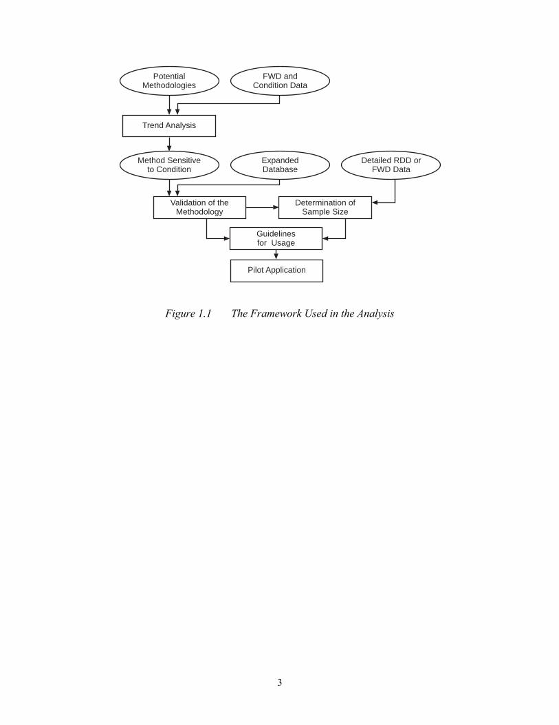
Figure 1.1 The Framework Used in the Analysis......................................................................3
Figure 2.1 Stress Distribution and Measured Deflection Bowl Beneath FWD Load [Rohde 1994] ...............................................................................................11
Figure 3.1 Deterioration Process of a Pavement Over Time...................................................16
Figure 3.2 Used vs. Not-Used Data Points From Initial Sample ............................................19
Figure 3.3 Correlation Between SN Estimates From Methods III and IV..............................22
Figure 3.4 Relationship of the Deflection Ratio (W7/W1) and Modulus Ratio Ep/Mr ......................................................................................................................23
Figure 3.5 Relationship of Pavement Modulus and Structural Number in Method III ...........................................................................................................................23
Figure 4.1 Environmental Zones and District Boundaries ......................................................26
Figure 4.2 Relationship of SN Using Method IV and SN Using Backcalculated Moduli for Selected ID Sections............................................................................29
Figure 5.1 Distribution of the ESALs .....................................................................................33
Figure 5.2 Distribution of Squared Resilient Subgrade Modulus (Mr) ...................................34
Figure 5.3 Distribution of the Structural Condition Index ......................................................36
Figure 6.1 The Trade-Off Between Testing Costs and Failure Rate.......................................40
Figure 6.2 Typical Limit of Accuracy Curve for All Pavement Variables Showing General Zones [AASHTO 1993] ............................................................41
Figure 6.3 Histogram of the CV for 60 Sections Considered in the Analysis ........................45
Figure 6.4 Histogram of the LOG CV for 60 Sections Considered in the Analysis ...............45
Figure 8.1 The Pavement Structures of the Subsections for FM 762 .....................................52
Figure 8.2 The SCI and Distress Score Values for Section FM 762.......................................53
Figure 8.3 Distribution of the SCI Values for Section FM 762 ..............................................54
Figure 8.4 Cumulative Distribution of the SCI Values for Section FM 762 ..........................54
Figure 8.5 Distribution of the SCI Values for the FM 762 Middle Subsection ......................55

x
Figure 8.6 Cumulative Distribution of the SCI Values for the FM 762 Middle Subsection..............................................................................................................55
Figure 8.7 The SCI and Distress Scores for Section FM 1463 ...............................................56
Figure 8.8 Distribution of the SCI Values for Section FM 1463 ............................................57
Figure 8.9 Cumulative Distribution of the SCI Values for Section FM 1463 ........................57
Figure 8.10 The SCI and Distress Score Values for Section FM 1640.....................................58
Figure 8.11 Distribution of the SCI Values for Section FM 1640 ............................................59
Figure 8.12 Cumulative Distribution of SCI Values for Section FM 1463 ..............................59

xi
List of Tables
Table 2.1 Coefficients for SN Versus SIP Relationship [Rohde 1994] .................................12
Table 3.1 Required Input Information and the Corresponding Structural Estimators for Each Method .................................................................................15
Table 3.2 Type of Pavements Description in TxDOT PMIS.................................................18
Table 3.3 Factorial Design Table...........................................................................................20
Table 3.4 Number of ID Sections Considered in the Analysis ..............................................21
Table 3.5 The Layer Coefficients Used in the Comparison Analysis....................................24
Table 3.6 Real SN Values and SN Values from Methods III and IV ....................................24
Table 4.1 Effects of the Environmental Zones on Yearly Ride Score Deterioration (dRS), Resilient Subgrade Modulus (Mr), Structural Number (SN), and ESALs .....................................................................................27
Table 4.2 Values of SN Using Method IV and From Backcalculated Layer Moduli....................................................................................................................28
Table 4.3 The Sections with the Accurate Total Thickness Information ..............................28
Table 5.1 Required SN for Different Categories of Accumulated ESAL Traffic and Mr. ...................................................................................................................35
Table 5.2 Alternative Limits of the Mr and 20-Year Accumulated Traffic in ESALs ....................................................................................................................35
Table 6.1 Summary of Mean, Standard Deviations and Coefficients of Variances of the Existing SN for 60 Sections.........................................................................43
Table 6.2 Average Standard Deviation for Asphalt Concrete Pavement Thickness From New Jersey ..................................................................................44
Table 6.3 Number of Samples for Different Confidence Levels (CI) and Allowable Error (e) on Half-Mile Sections ...........................................................46
Table 7.1 Coefficients for Determining the SN .....................................................................48
Table 7.2 Required SN for Different Categories of Accumulated ESAL Traffic and Mr ....................................................................................................................49


1
1. Introduction
1.1 Background Over the years many state highway agencies, including the Texas Department of
Transportation (TxDOT), in order to preserve the large highway network, have applied extensive seal coats, thin overlays, and other types of surface treatments to improve the surface conditions and seal existing cracks.
Those measures have provided a temporary improvement of surface conditions, but they did not provide the remedy to any structural deficiency associated with the pavements. Huge amounts of seal coats and thin overlays that had been applied every year have not prevented the problem from reoccurring. As a result, the overall pavement condition kept deteriorating due to the structural deformation of pavement layers and the subgrade, even though surface treatments were applied periodically.
To make proper decisions about the type of treatment needed, one should consider characterizing the pavement structural condition. The structural condition of the pavement can be assessed using several different measurements, but the most comprehensive approach would be using falling weight deflectometer (FWD) data. The FWD is widely used by the Texas Department of Transportation (TxDOT) as a type of non-destructive testing (NDT) for structural evaluation of pavements. The Pavement Management Information System (PMIS) stores this data. The falling weight deflectometer (FWD) measures deflections when known impulse loads have been induced on the pavement to be examined. FWD data are commonly used for backcalculation of the layer’s moduli.
Even though TxDOT collects and stores FWD data in the PMIS, this backcalculation procedure cannot be used because the PMIS does not contain the thickness information for the pavement layers at the present time. Instead, the PMIS has only an estimated total thickness for each section of the pavements [TxDOT 2000].
According to the statistics from the TxDOT PMIS, the ride score (RS) of the highway network in Texas is decreasing at an average of 0.3 score points a year. The decrease in the ride score is due to the increase in pavement roughness caused by the permanent deformation of the pavement structure. The deformations are the result of inadequate pavement strength for the existing traffic load. Therefore, there is an urgent need for an effective pavement structural index that could discriminate between pavements requiring additional strength through overlays, rehabilitation, or reconstruction and those for which surface treatments would be sufficient.
To overcome the problem of estimating the structural condition of the pavement using FWD data without information about the thickness of each layer, the TxDOT PMIS stores a structural screening parameter called the Structural Strength Index (SSI) [Scullion 1988]. Recent internal studies at TxDOT indicated that the SSI was not sensitive enough to discriminate between pavements that need structural reinforcement from those that do not.
1.2 Estimating Structural Condition of Pavements As more comprehensive studies were conducted in highway design and in pavement
design in particular, researchers have proposed a number of methodologies for estimating

2
the structural condition of pavements. The pavement structural condition is primarily characterized by the modulus of a pavement or by the Structural Number (SN) of a pavement.
The SN is a direct product resulting from the AASHO Road Test, the most comprehensive research on pavements conducted in the United States. Following the completion of the Road Test, the AASHO Design Committee developed the AASHO Interim Guide for the Design of Rigid and Flexible Pavements, where the Structural Number is used as the indicator of the strength of a pavement [AASHTO 1993].
1.3 Objectives and Scope of the Research The main objective of the research was to develop a structural index, based on the
FWD data, that would be able to discriminate between pavements requiring additional structural capacity and those for which surface treatments would be sufficient. The limiting requirement for such an index was that it should provide a general indication of the structural adequacy of a pavement based on the estimated total thickness of the pavement, as the actual layer-by-layer thickness of pavements was not available at TxDOT.
In addition, a contingent sampling procedure was developed to determine the minimum number of FWD tests required for each management section of pavements. Subsequently, comprehensive guidelines were developed for using the SCI in the selection of the best maintenance and rehabilitation alternatives at network level.
Finally, a pilot application of the SCI was carried out with several pavement rehabilitation projects to verify the validity of the SCI. The intention was to apply the modifications to the developed procedure if such a need was determined from the pilot application.
1.4 Framework Used in the Analysis The methodology is based on a sequential analysis process, as illustrated in Figure
1.1. First, an assessment of the potential methods that can be used for the structural evaluation of the pavements was considered, through the assessment of the input data that are available from the TxDOT PMIS. Second, the trend analyses were conduced and the conclusions about the sensitivity of the methods were made. Then the validation of the trends established in the previous step, along with the overall methodology validation, was conducted using an expanded database. Next, the statistical analysis process for determining sample size (sampling frequency) was developed. Finally, guidelines and recommendations for using the SCI were developed and validated with the real pilot project application.
3
PotentialMethodologies
FWD andCondition Data
ExpandedDatabase
Detailed RDD orFWD Data
Method Sensitiveto Condition
Trend Analysis
Validation of theMethodology
Determination ofSample Size
Guidelinesfor Usage
Pilot Application
Figure 1.1 The Framework Used in the Analysis


5
2. Overview of the Methods for Estimating Structural Condition of Pavements from FWD Data
2.1 Introduction Several existing methods for determining the structural condition of pavements were
reviewed for possible implementation in this study. These methods are discussed in more detail in the following sections. One of the key criteria in the selection process was the availability of data currently stored in the TxDOT PMIS. Such a criterion has helped reduce the number of feasible methods to those that require only the deflection data and total thickness of a pavement. The output of such methods was the modulus (Ep) or the Structural Number (SN) of the pavement.
Using the above defined criterion, five different methods were selected:
a) Method I – The Modulus and Deflection Ratios.
b) Method II – The Modified Modulus and Deflection Ratios.
c) Method III – The Method Using Structural Number.
d) Method IV – An Alternative Method for Determining SN from FWD Data.
e) Method V – Simple Approach Method to Estimation of Pavement Structural Capacity.
2.2 The Current Structural Index Used by TxDOT The current pavement structural index used in the TxDOT PMIS is the statistical
Structural Strength Index (SSI) developed by the Texas Transportation Institute (TTI) [Scullion 1988]. The SSI was developed based on the Surface Curvature Index (SCI) and the Falling Weight Deflectometer (FWD) deflection of Sensor 7 (W7), which is 72 inches away from the center of the applied FWD loading. The deflections are normally measured under an approximately 9,000 lb load with seven sensors (geophones) that are spaced 12 inches apart. The SCI is expressed as the difference between the deflection from the first sensor (W1) and that from the second sensor (W2):
SCI = W1 – W2
The SSI is calculated as a function of the SCI and W7 according to two tables, one for thin asphalt pavements and the other for intermediate and thick asphalt pavements [Scullion 1988]. The Statistical Structural Strength Index (SSIF) is then calculated by incorporating the rainfall factor (RF) and traffic factor (TF) into the index:
SSIF = 100 * SSI / (RF * TF)
The SSI was added to the Pavement Evaluation System (PES), which preceded PMIS, in October 1987. In April 2000, TxDOT conducted an internal study and applied

6
the SSI for two highways in Texas: US-79 in the Bryan District and US-77 in the Pharr District. US-79 was in very good condition as it was reconstructed; whereas, US-77 had substantial amounts of distress such as alligator cracking, pumping, and rutting. In other words, the conditions of the two highways were significantly different. However, the results from the study indicated that the calculated SSI values at an 85 percent confidence interval for the two highways were not very different: 90 for US-79 and 79 for US-77.
This means that the current SSI is not sensitive enough to discriminate one highway from another even if there is a significant difference in the structural capacity between the two highways. In other words, the SSI cannot be effectively used at the network level to identify pavement sections with structural deficiencies.
Furthermore, the SSI does not relate the FWD values to the structural capacity indicators, such as the Structural Number (SN), that are used for pavement design. Therefore, it is hard to decide whether a pavement needs strengthening or surface treatment just by looking at the SSI values. It is clear that an alternative method is needed in order to overcome the problems associated with the current structural index.
2.3 Method I – The Modulus and Deflection Ratios The modulus and deflection ratios method consists of two parts. The first part is the
analysis of the modulus of a pavement structure as a whole in relation to the subgrade modulus using the ratio of W1/W7, representing the ratio of pavement modulus and subgrade modulus. The deflection reading at the center of loading (W1) gives the stiffness of the pavement and the subgrade, and (W7) the stiffness of the subgrade only. The calculated modulus of the whole pavement is then compared to the required pavement modulus.
The second part of the method is intended to identify weak layers in pavements by using the ratios of FWD deflections such as W2/W1, W3/W2, W4/W3, W5/W4, W6/W5, and W7/W6. The minimum ratio would indicate a layer that is weaker than the other pavement layers. For example, a very small W3/W2 ratio indicates that the base layer is significantly weaker than the surface layer. The following equations for calculating the existing pavement modulus (Ep) are adopted from an unpublished TxDOT Technical Memorandum summarizing an internal study conducted by Claros in April 2000. The existing pavement modulus is calculated as follows:
a) Calculate the ratio of W7/W1 for each deflection basin.
b) Calculate the estimated subgrade resilient modulus [AASHTO 1993]:
Esubgrade = 0.24 * P/(W7 * 72) where Esubgrade = backcalculated subgrade resilient modulus in psi. P = applied load in pounds. W7 = deflection at sensor 7 in inches.
c) Calculate the ratio of the pavement modulus to the subgrade modulus using the regression equations provided by Wimsatt in (1998, 1999), where selection of the

7
equations is determined by the total thickness of the pavement. An example of the equation for a 21-inch pavement is given as the following:
Ep/Esubgrade = 516.94 * (W7/W1)5/2 – 214.46 * (W7/W1)2 + 159.56 * (W7/W1)3/2 –
6.143 * (W7/W1) + 1.0826 * (W7/W1)1/2
d) Calculate the existing pavement modulus Ep:
Ep = (Ep/Esubgrade) * (Esubgrade)
e) Determine the design pavement modulus:
Edesign = (500*DACP + 60*DFB + 45*DLT)/ DTotal where Edesign = the design modulus of the pavement, in ksi. DACP = the depth of the asphalt pavement layer, in inches. DFB = the depth of the flexible base layer, in inches. DLT = the depth of the lime-treated subbase layer, in inches. DTotal = the total depth of pavement layers, in inches.
f) Compare the existing pavement modulus (Ep) to the design pavement modulus (Edesign) for sections with inadequate structural capacity.
According to the TxDOT internal analysis, this method is sensitive enough to
differentiate pavements that need additional structural capacity from those that do not. However, certain improvements were needed for the method to be implemented for network-level applications. These improvements include:
a) Simplification is needed to reduce the fifth degree polynomial equations.
b) The layer thicknesses required for determining the design pavement modulus are not currently available. In addition, the required design pavement modulus should be a function of the existing traffic, future traffic and environmental conditions.
c) A ratio of the existing pavement modulus to the required design pavement modulus should be developed so that threshold values can be established to define pavements requiring additional strengthening.
2.4 Method II – The Modified Modulus and Deflection Ratios The modified modulus and deflection ratios method is a modification of the method
presented in the previous section. The procedure is composed of following steps:
a) Calculate the ratio of W7/W1 for each deflection basin.

8
b) Calculate the estimated subgrade resilient modulus (Esubgrade):
Esubgrade = 0.24 * P / (W7 * 72) where Esubgrade = backcalculated subgrade resilient modulus in psi. P = applied load in pounds. W7 = deflection at sensor 7 in inches.
c) Calculate the ratio of the pavement modulus to the subgrade modulus using the regression equations. An example of the equation for a 21-inch pavement is given as the following:
Ep/Esubgrade = - 1.8497 + 29.952 * (W7/W1)0.5 – 124.62 * (W7/W1) + 331.3 *
(W7/W1)1.5
d) Calculate the existing pavement modulus Ep:
Ep = (Ep/ Esubgrade) * (Esubgrade)
e) Determine the required design pavement modulus for the existing subgrade modulus and the expected future ESALs :
Erequired = 6.06 * 106 * [(ESAL)0.307/(Esubgrade)1.6881] where Erequired = the required design modulus of the pavement. ESAL = accumulated ESALs for the design period. Esubgrade = backcalculated subgrade modulus in psi at 85% CI.
f) Calculate the ratio of the existing pavement modulus (Ep) to the required design pavement modulus (Edesign) at 85 % confidence interval (CI).
Ratio (at 85% CI) = Mean Ratio – 1.04 * (Standard Deviation).
g) Determine the sections requiring additional structural capacity using the following criteria:
Ratio (at 85% CI) < 0.5: urgent strengthening is required. 0.5 ≤ Ratio (at 85% CI) < 1.0: strengthening may be needed in the future. Ratio (at 85% CI) ≥ 1.0: strengthening is not required.
It is clear that the modified method has several advantages over the original method. It is easier to calculate and it takes into consideration the required design modulus for the

9
ESALs and environmental conditions. The new ratio can be directly used to identify pavement sections requiring strengthening. As in the original method, the modified method can calculate the minimum values of deflection ratios to be used in identifying the potential weakness of the base layer. The main drawback of this modified method is that it does not relate to the SN value used in pavement design.
2.5 Method III – The Method Using Structural Number The analysis presented by Wimsatt (1998, 1999) is based on the assessment of the
modulus of the pavement structure as a whole in relation to the subgrade modulus using the ratio of W7 to W1 (W7/W1), which is the ratio of pavement modulus to subgrade modulus. The deflection underneath the loading plate W1 gives the stiffness of the pavement and the subgrade; whereas, the deflection 72 inches away from the plate (W7) gives the stiffness of the subgrade only.
The pavement to subgrade modulus ratio (Ep/Esubgrade) can be calculated from the regression equations developed by Wimsatt (1998). Such equations are functions of (W7/W1) and the subgrade modulus. Subgrade modulus can be estimated using the equation from the AASHTO Guide for Design of Pavement Structures.
Esubgrade = 0.24 * P/(W7 * 72)
where Esubgrade = backcalculated subgrade resilient modulus in psi. P = applied load in pounds. W7 = deflection at sensor 7 in inches.
The pavement to subgrade modulus ratio regression equation for 21-inch pavements
is presented below:
Ep/Esubgrade = 516.94 * (W7/W1)5/2 – 214.46 * (W7/W1)2 + 159.56 * (W7/W1)3/2 – 6.143 * (W7/W1) + 1.0826 * (W7/W1)1/2
where (Ep/ Esubgrade) = pavement to subgrade modulus ratio. W1 = deflection at sensor 1 in inches. W7 = deflection at sensor 7 in inches.
The existing pavement modulus Ep is calculated using following expression:
Ep = (Ep/Esubgrade) * (Esubgrade)
The calculated modulus of the whole pavement is then compared to the required
pavement modulus to see if the pavement is structurally adequate. This is a different approach from that presented in the AASHTO Guide for Design of
Pavement Structures, where the pavement modulus is calculated from an equation that can be solved only through numerical-iterative methods.

10
The use of a complicated iterative equation is a major setback in the implementation of such a procedure. For this reason, this research focused on using the equations developed by Wimsatt (1998). The programming required for the implementation of such a procedure would not constitute a significant problem.
With known values of pavement modulus and total thickness, one could estimate the structural number using the following relationship [AASHTO 1993]:
SNeff = 0.0045 * D * Ep
0.333
where D = total thickness of the pavement layers. Ep = existing pavement modulus of all layers above the subgrade.
Apparently, it is not feasible to characterize the adequacy of a pavement by using
only the estimated effective SN. In order to evaluate the pavement’s structural adequacy, one needs the required SN. With the required and the effective SN, the structural deficiency can be characterized as the difference between the required and the effective SN.
2.6 Method IV – An Alternative Method for Determining SN from FWD Data The peak deflection represented by an FWD bowl is a combination of the deflection
in the subgrade and the elastic compression of the pavement structure. Irwin (1983) suggested a rule based on the fact that 95 percent of the deflections measured on the surface of a pavement originate below a line deviating 34 degrees from the horizontal. This is illustrated in Figure 2.1.

11
OFFSET
SUBGRADE
FWD LOADPLATE
FWD SENSORS
SURFACE
BASE ANDPAVEMENTLAYERS
FWD STRESSDISTRIBUTION
FWD DEFLECTION BOWL
SIP
SIS
Hp
1.5 Hp
YO
450 mm
34˚
CL
Figure 2.1 Stress Distribution and Measured Deflection Bowl Beneath FWD Load [Rohde 1994]
With this simplification, Rohde (1994) concluded that the surface deflections measured at an offset of 1.5 times the pavement thickness originate entirely in the subgrade. By comparing this deflection with the peak deflection index (SIP), one can define the amount of deflection that originated from within the pavement structure only.
SIP = W1 – W1.5Hp
where SIP = structural index of pavement (microns, where 1 micron = 1/1000th of a
millimeter). W1 = peak deflection measured under a standard 9,000-lb FWD load (microns). W1.5Hp = surface deflection measured at offset of 1.5 times of Hp under a
standard 9,000-lb FWD load (microns). Hp = total pavement thickness (which does not include stabilized subgrade)
(mm).
The Structural Number of the pavement was calculated knowing the total pavement thickness and the value of SIP. The function below was used in the analysis.

12
SN = k1 * SIPk2 * Hp
k3 where SN = pavement structural number (in). SIP = structural index of pavement (microns). Hp = total pavement thickness (mm). k1, k2, k3 = regression coefficients, listed in Table 2.1.
Table 2.1 Coefficients for SN Versus SIP Relationship [Rohde 1994]
Surface Type k1 k2 k3 r2* n** Surface Seals 0.1165 -0.3248 0.8241 0.984 1944
Asphalt Concrete 0.4728 -0.4810 0.7581 0.957 5832 * Coefficient of Determination ** Sample Size
The procedure for calculating the Structural Number (SN) from the deflection data
using methodology based on the “two-third” rule is fairly simple and easily implementable in the PMIS. The overall accuracy of the method is discussed by Rohde (1994).
2.7 Method V – Simple Approach Method to Estimate the SN of Pavements This method proposed by Romanoschi and Metcalf (1999) gives a direct regression
relationship between the measured FWD deflection and the structural strength of the pavement, expressed as the pavement’s Structural Number (SN).
The Structural Number (SN) regression equations were expressed separately for pavement structures having granular base and subbase layers, and for pavement structures having a stabilized base layer.
a) For the pavement structure with cement treated layers:
SN = 6.45 – 3.676 * log(D0) + 3.727 * log(D1500) where SN = structural number. D0 = temperature corrected central deflection (microns). D1500 = deflection at an offset of 1500 mm (60 in). D1500 = D600 – 3 * D900 + 3 * D1200. where D600 = deflection at an offset of 600 mm (24 in). D900 = deflection at an offset of 900 mm (36 in). D1200 = deflection at an offset of 1200 mm (48 in).

13
The regression is relatively poor (R2 = 0.436), but the standard error of the SN estimation is 0.454.
b) For the pavement structure without cement treated layers:
SN = 6.96 – 0.196 * [(AREA) – 450 * (D1200)]0.5
where AREA = 25.48 * [4 * D0 + 6 * D200 + 5 * D300 + D450]. D0 = temperature corrected central deflection (microns). D200 = deflection at an offset of 200 mm (8 in). D300 = deflection at an offset of 300 mm (12 in). D450 = deflection at an offset of 450 mm (18 in).
The regression is relatively good (R2 = 0.762), and the standard error of SN
estimation is 0.273.
2.8 Summary of the Methods Being Reviewed In order to evaluate which of the proposed methods is the most suitable for the
implementation in the PMIS, further analyses are needed. Method I or Modulus and Deflection Ratios is not suitable since it requires the layer-by-layer thickness of the pavement. Such information was not available from data sources at the TxDOT. During the preliminary analysis, the estimates of SN from Method V did not fall under the normal range of the SN values. The method yielded negative or unrealistically big values of the SN, such as 100 or more. Consequently, the conclusion from the preliminary analysis was that Method V was also unsuitable for further evaluation.
Methods II, III and IV have satisfied all the data limitation from the problem statement, and showed reasonable estimates of SN in the preliminary analysis. Therefore, they were further examined with regard to suitability for the implementation in the PMIS as discussed in the following chapters in detail.


15
3. Sensitivity Analysis of Pavement Structural Estimators to Condition Indicators
3.1 Methodology In order to qualitatively characterize the proposed methods for describing the
structural condition of the pavement, it was necessary to conduct an analysis to determine how sensitive the structural estimators are to the condition measurements stored in the TxDOT PMIS. The Table 3.1 shows the required input information for each method and the structural estimator as an output.
Table 3.1 Required Input Information and the Corresponding Structural Estimators for Each Method
METHODS I II III IV V
W0 X X X X X W8 X X W12 X X W18 X X W24 X W36 X W48 X X W60 X X
FWD
W72 X X X X DT X X X Thickness Di X a X p X P X X X
INPU
T
Other
ESAL X X Ep X
Edesign X Ratio (Ep/Erequired) at 85 %
CI X
OU
TPU
T
SN X X X
3.1.1 Pavement Deterioration Variables In order to identify the best methodology for determining structural estimators that
can be used to qualitatively assess different pavement structural conditions, one has to consider the deterioration process of the pavement. The TxDOT PMIS stores three score values that describe the quality of pavements [TxDOT 2000]:

16
a) Distress Score. It describes the amount of visible surface deterioration pavement
distress. The values range from 1 (most distress) to 100 (least distress).
b) Ride Score. It describes a pavement’s roughness. The Ride Score ranges from 0.1 (roughest) to 5.0 (smoothest).
c) Condition Score. It describes a pavement’s overall condition in terms of distress and ride quality (SI values). Condition Score values range from 1 (worst condition) to 100 (best condition).
The surface condition of a pavement is implicitly correlated with the structural
condition. It is common knowledge that pavements become much more susceptible to the deterioration process when their structural condition is poor.
The deterioration process of a pavement represents the behavior of a non-linear system and it can be characterized by different rates of deterioration in different stages of the pavement service life. The typical deterioration of the PSI value of a pavement during the life cycle is shown in Figure 3.1.
Unit of Time
dPSI
dPSIPSI
Time
Unit of Time
Figure 3.1 Deterioration Process of a Pavement Over Time
It is known that the roughness of a pavement contributes significantly to the PSI values [AASHTO 1993]. The TxDOT PMIS does not use PSI values directly; rather it uses the Ride Score as the roughness measurement. It is fair to assume that the Ride Score is positively correlated to the PSI value.
Naturally, the true condition of a pavement at any moment can be described more accurately if the deterioration rate is known. Unfortunately, a mathematical solution to this problem is impossible because there are no models that can precisely represent the true deterioration process of a pavement. Even complicated mathematical models such as sigmoid forms can not be calibrated accurately enough to represent a true deterioration process. If the general mathematical formula describing the transition of a system from one state to another is not available, one can use the finite difference between the states. By

17
doing so, even though the estimate will not be very accurate, it will establish a general trend.
The yearly difference between score values, or the change over a unit time, represents the rate of deterioration. Furthermore, if the difference is normalized by its initial condition, it would give a more accurate picture of the pavement deterioration process. For example, a big drop in the score value at the beginning of the pavement life would represent different pavement structural conditions than one where the same drop occurred at the end of its life.
Another important factor in characterizing a pavement deterioration process is the traffic. For pavement design, traffic is generally expressed in terms of the Equivalent Single Axle Load (ESAL). An equal yearly drop in the condition score of a pavement subjected to different ESALs represents different structural conditions of the pavement. For example, without considering traffic, the same drop in score values for two different pavement sections would mean the same structural condition of the pavement; whereas in fact, the drop for one section was caused by much greater traffic loading. It is obvious that the pavement that carries more ESALs is structurally better than the other.
If the normalized drop in score values is divided with the yearly traffic in ESALs, a more accurate structural condition of the pavement at the time of the FWD testing can be obtained. This also can be viewed as a unit deterioration of the PMIS score values caused by a single ESAL load. It can be expected that the pavements with sound structural conditions would give smaller values of the Unit ESAL Deterioration (UED), than the ones that are not in sound structural conditions.
In the analysis conducted by the researchers, the Unit ESAL Deterioration (UED) is calculated as the normalized yearly drop in the PMIS scores (Ride, Condition and Distress Scores), caused by a single ESAL for a consecutive two-year period:
6
y10×
ESAL×DSdDS
=) Score Distress ( UED
6
y10×
ESAL×CSdCS
=) ScoreCondition ( UED
6
y10×
ESAL×RSdRS
=) Score Ride ( UED
where DS = Distress Score in initial year. RS = Ride Score in initial year. CS = Condition Score in Initial year. dDS = yearly drop in Distress Score. dCS = yearly drop in Condition Score. dRS = yearly drop in Ride Score. ESALy = estimated amount of ESALs in a year.

18
Structural deterioration is defined as any process that reduces the load-carrying capacity of the pavements. It can be observed that a structural failure occurs when the roughness starts progressing at a greater rate. Some pavements may have been constructed with a poor initial roughness condition, but with a perfect structural condition. Such scenarios suggest that the use of a UED would be more appropriate, since those pavements would experience a smaller rate of deterioration than the ones constructed with a poor structural condition.
3.2 Data Used in the Analysis An initial sensitivity analysis of the field condition measurements with respect to the
pavement’s structural estimators was performed using the PMIS database from the district with the most FWD data in PMIS−the Fort Worth district. The data set that was available in the study included the PMIS data from fiscal years 2000 and 2001.
Sections were identified by the highway PMIS code and the beginning and the ending location. Those sections that did not have complete information were eliminated. The required information for the analysis was the condition and the deflection measurements for at least two consecutive fiscal years.
The processing of the Fort Worth district PMIS yielded a database of 2,192 data points, with all the necessary information for the analysis. The database includes sections from more than 10 counties in the district.
Table 3.2 shows types of pavements and the corresponding specific codes. Most of the data used in the analysis came from detailed types: 04, 05, 06, 08, and 10. Since the objective of the project is to obtain structural estimators without prior knowledge of the thickness of the pavement layers, the researchers did not take into account the information about the particular type and thickness of layers. Table 3.2 shows the type of codes used in the PMIS. The only relevant information used was the definition of a pavement type. For example, for asphalt-concrete pavements, the code was A.
Table 3.2 Type of Pavements Description in TxDOT PMIS
Detail Detail Pavement Type Long Pavement 01 01 – Continuously Reinforced Concrete Pavement C 02 02 – Jointed Reinforced Concrete Pavement J 03 03 – Jointed Plain Concrete Pavement J 04 04 – Thick Asphalitc Concrete Pavement (greater then 5½") A 05 05 – Intermediate Thickness Asphaltic Concrete Pavement A 06 06 – Thin Surfaced Flexible Base Pavement (less than 2½") A 07 07 – Composite Pavement (Asphalt Surfaced Concrete Pavement) A 08 08 – Overlaid and/or Widened Old Concrete Pavement A 09 09 – Overlaid and/or Widened Old Flexible Pavement A 10 10 – Thin Surfaced Flexible Base Pavement (Surface Treatment) A

19
All the data points were from one environmental zone, defined as Wet-Cold, although the Fort Worth district neighbors two other zones: Mixed and Dry-Cold. The traffic was defined in ESALs and it ranged from 1,100 to 988,350 yearly loadings (CURRENT_18KIP_MEAS as defined in the database divided by 20).
In order to have analyses that yield more reliable results, the researchers needed to define the factors that influenced the behavior of variables. Ideally all of those variables needed to be recorded. Unfortunately the PMIS database did not have maintenance records for each section, so the researchers could not determine which sections received maintenance work. In order to overcome this, the difference in Ride Score for two consecutive years was used as an indicator. A positive difference in the Ride Score indicates (i.e., RS 2000 – RS 2001) with a great probability that the section did not receive any maintenance that was applied to improve the ride quality; whereas, a negative difference would indicate that some type of maintenance work was applied to the pavement. It is important to note that no information was available to detect maintenance actions that did not effect ride quality, like crack seals. Another important issue related to the approach is the accuracy of the measurements and the time frame of consecutive measurements. The average accuracy of Ride Score is about two units of measurements. A one-year time frame assures that if there were a drop in the Ride Score, the section did not receive any maintenance work. This is because it is highly unlikely that for one year a pavement that has received some maintenance work could deteriorate below its pre-intervention Ride Score value.
An initial data set was formed from the 2,192 data points. The reduction of the data was performed under the condition that the difference in Ride Score values has to be positive, providing a new data set for the analysis. Figure 3.2 shows the proportion of the data points used in the analysis and those excluded because of the negative difference in the condition scores.
NotUsed952
Used1,240
Figure 3.2 Used vs. Not-Used Data Points From Initial Sample

20
3.3 Factorial Design In order to obtain more reliable results that would indicate which of the methods is
the most sensitive to the field data, a factorial design was developed. Variables used for the factorial design were RS, dRS, dRS/RS, UED (RS), CS, dCS, dCS/CS, and UED (CS). The RS indicates the initial score value for the first of two consecutive years. Since the Distress Score showed almost an identical trend as the Condition Score, it was omitted from the factorial design. The response variables were structural estimators Ep and SN. To differentiate between various categories of pavements, the total thickness of pavements was used. Table 3.3 gives a summary of all the factors considered. The “X” indicates that a trend analysis was conducted for the particular factor. Therefore, the table shows that the trend analysis was conducted for the data stratified by the pavement thickness. The column marked as “ALL” indicates that the trend was plotted when data with different thicknesses was combined together.
Table 3.3 Factorial Design Table
Methods Existing Tool
Method II (Ep)
Method III (SN)
Method IV (SN)
SSI
Considered Total Thickness (inches)
RS 9 12 15 ALL 9 12 15 ALL 9 12 15 ALL 9 12 15 ALL
CS X X X X X X X X X X
dRS X X X X X X X X X X
dCS X X X X X X X X X X
dRS/RS X X X X X X X X X X
dCS/CS X X X X X X X X X X
UED (RS) X X X X X X X X X X
UED (CS) X X X X X X X X X X
Table 3.4 gives the number of data points available when each factor was stratified
by the total thickness obtained from the TxDOT PMIS..

21
Table 3.4 Number of ID Sections Considered in the Analysis
Thickness of ID Sections Stratification of Factorial Design 9 12 15 ALL
(dRS/RS) 747 407 86 1,240
(dCS/CS) 747 407 86 1,240
UED (RS) 747 407 86 1,240
UED (CS) 747 407 86 1,240
Method I or Modulus and Deflection Ratios was not included in the analysis because
it requires the thickness of each layer. Method II or Modified Modulus and Deflection Ratios was used up to a certain degree when the value of pavement modulus was determined. Further analysis using this method was not possible since the information about the design ESAL was not available. Method V gave the SN estimates that did not fall in the range of “reasonable” values (such as negative SNs or SNs values above 100), and therefore it was disregarded.
3.4 Findings and Directions for Further Analysis Different factors, such as dRS, dCS/CS or UED(RS) have shown different levels of
sensitivity to the structural estimators, but the outputs from all considered methods have shown some level of sensitivity to the UED values. As the deterioration increases, the structural estimators tend to produce smaller values. When the data were stratified by the thickness, it produced a better trend, but with a greater variance. The trend plots are summarized in Appendix A.
The factor defined as UED(RS) has shown the best trend for all methods. Among the three methods considered, Method III and Method IV yielded the best and very similar trends as illustrated by Figures A.1 to A.25 in Appendix A. The intention of the trend analyses were to visualize whether there was a trend between the deterioration variables, like Unit ESAL Deterioration (UED) of the PMIS score values, and the pavement structural estimators (Ep and SN). However, it was not intention of this study to quantify the correlation between them through regression analysis or other similar means.
In addition to these methodologies, the current index of estimating structural capacity of a pavement (SSI) was calculated. The SSI did not show any sensitivity to those factors considered in the analysis.
3.4.1 Qualitative Assessments of the Considered Methods Among the three methods, Method III and Method IV are directly related to the SN
values, and therefore can be easily used to evaluate maintenance or rehabilitation (M&R) options. For example, correction of a SN deficiency is an option in AASHTO design [ASSHTO 1993]. Having that in mind, the researchers focused on those two methods. The analysis has shown some correlation between SN estimates from two methods; however, one produced greater SN estimates than the other. The two methods demonstrate an almost

22
linear relationship. For example, if the relationship between the estimates of the SN is assumed linear, then the regression analysis shows that the estimate from Method IV is about 56 percent greater than that from Method III. The linear regression was performed with data excluding 3 sections with negative SN estimates, yielding the coefficient of determination (R2) of 0.92. This is shown in Figure 3.3.
16
14
12
10
8
6
4
2
0
-4 -2 0 2 4 6 8 10
Structural Number from Method III (SN) III
Str
uctu
ral N
umbe
r fr
om M
etho
d IV
,S
N (
IV)
SN (IV) = 1.5602 SN (III) - 0.0048
R2 = 0.92
Figure 3.3 Correlation Between SN Estimates From Methods III and IV
It can be observed from Figure 3.3 that Method III has yielded negative SN estimates for 3 sections. For W7/W1 deflection ratios smaller than 0.006, the polynomial regression equation for estimating the ratio of Pavement Modulus and Modulus of Subgrade (Ep/Mr) produced negative values. Subsequently, further calculations produced negative values of the Structural Number (SN). This is the case only for the 9-inch pavements regression equations. The relationship between W7/W1 and Ep/Mr is shown in Figure 3.4. Furthermore, the effects of Ep/Mr, with the fixed value of the resilient subgrade modulus of Mr = 7,000 psi, to the values of the Structural Number (SN) estimates from Method III, are shown in Figure 3.5. As a result, another version of the regression equation for 9-inch pavements was tested, giving consistent results and the values of estimated SN above 0. However, it is valid only for the ratios of Pavement Modulus and Modulus of Subgrade (Ep/Mr) between 0.5 and 25.

23
0.4
0.2
0.0
-0.2
-0.4
-0.6
-0.8
0.000 0.002 0.004 0.006 0.008 0.010 0.012
Deflection Ratio (W7/W1)
For W7/W1 ratios less then 0.006 (H=9 inch) => Negative Ep/Esg
Mod
ulus
Rat
io E
p/M
r
Figure 3.4 Relationship of the Deflection Ratio (W7/W1) and Modulus Ratio Ep/Mr
0.8
0.6
0.4
0.2
0.0
-0.2
-0.4
-0.6
-0.8
-1.0
-5000 -4000 -3000 -2000 -1000 0 1000 2000 3000
Str
uctu
ral N
umbe
r (S
N)
Modulus Ratio Ep/Mr
Mr = 7000 psi
Figure 3.5 Relationship of Pavement Modulus and Structural Number in Method III
In order to determine which method gives more accurate SN estimates, the researchers have obtained more elaborate and complete data for certain pavement sections that were just constructed. The complete information enabled the researchers to calculate the standard SN using the procedure defined in AASHTO Guide for Design of Pavement

24
Structures. Section FM0004 K was constructed with 2 inches of Asphalt Concrete Pavement (ACP), on one-half of an inch of a seal coat and 11 inches of Cement Treated Flexible Base (CTFB). Section FM0051 K was constructed with 5 inches of ACP on the top of the 9 inches of CTFB, whereas the structure of Section FM0917 K was composed of one-half of an inch of a seal coat, 2 inches of Asphalt Concrete Pavement (ACP) and 9 inches of CTFB. Section FM1810 K was constructed with 7.5 inches of ACP on the top of 6 inches of flexible base and 12 inches of cement stabilized subgrade. Finally, the structure of Section FM2280 K included 2 inches of ACP and 6 inches of flexible base. The layer coefficients used in the analysis were assumed as given in Table 3.5
Table 3.5 The Layer Coefficients Used in the Comparison Analysis
Layer Material Layer Coefficient (a) Asphalt Concrete Pavement (ACP) 0.40
Cement Treated Flexible Base (CTFB) 0.35 Flexible Base (FB) 0.14
Cement Stabilized Subgrade (CSS) 0.05
Calculated SN values were compared to the values yielded from Method III and Method IV. Table 3.6 summarizes the results.
Table 3.6 Real SN Values and SN Values from Methods III and IV
ID section Average SN from Method III
Average SN from Method IV
SN from AASHTO Guide
FM0004 K 3.09 4.63 4.65 FM0051 K 3.33 5.29 5.15 FM0917 K 1.88 3.64 3.95 FM1810 K 2.39 2.85 4.44 FM2280 K 2.00 2.54 1.64
It can be seen that the SN values from Method IV give a better estimation of the real
SN values calculated when the thickness and the conditions of the layers are known. However, the comparison should be treated as tentative for the reason that only 5 sections were used. In addition, there is a big discrepancy in the SNs for one of the sections. This could be due to the incomplete thickness information. The sum of all layer thickness above the subgrade does not always match the total thickness obtained from the PMIS.
With the results presented in Table 3.6, and the fact that Method III requires the use of complicated regression formulae, additional analyses had focused on the sensitivity of the Method IV SN estimates on a larger data set. Method IV is fairly simple and can be easily programmed into the current PMIS.

25
4. Sensitivity of the Structural Number (SN) From Method IV to the PMIS Score Values
4.1 Introduction Since the attention is given to the Method IV for the reasons described in Chapter 3,
more detailed analyses were needed to observe the performance of Method IV with a larger set of data. By doing this, the validity of the method can be tested against different kinds of environments. Since the data set from the Forth Worth district is the most complete set of data available, it was used as the benchmark data set for the initial screening of the methods under evaluation. The expanded data set that contains more districts was then used to validate the adopted method.
4.2 Definition of Larger Data Set The TxDOT PMIS database for the fiscal years 2000, 2001, and 2002 includes the
total of 13,522 sections with matching deflection and the condition data. Among them many sections have shown an actual increase in the PMIS score values, from the previous year to the next. Often, such an increase is an indicator that the sections have received some kind of maintenance action in between these two years. In order to obtain the data set usable for trend analyses, the initial expanded data set with a total of 13,522 sections was subjected to the same criteria as defined for the Fort Worth data set in Chapter 3. The only difference from the data set defined in Chapter 3 is that the expanded data set includes sections where the difference in the Ride Score for two consecutive years (dRS) is equal or greater than 0, as opposed to just being greater than 0. At the same time, the sections where the difference in the Condition Score (dCS) was less than 0 were excluded. Finally, a total of 7,460 sections have satisfied the above criteria and it was used in the validation procedure.
The condition for a difference in Condition Score greater than or equal to 0 indicates that the condition measurements of a particular pavement have actually decreased or stayed the same over a one-year time frame. The criterion was adopted in order to avoid the cases when the Ride Score condition has decreased over the one-year time frame, but at the same time for the same section, the Condition Score has increased.
The one-year time frame was defined as 2002 to 2001 and 2001 to 2000, as opposed to just 2001 to 2000 in the initial sensitivity analysis. This is because the initial data set from the Fort Worth district did not have the data for year 2002.
The new data set includes sections from all of the five Texas environmental zones, although some environmental zones include more sections than others.

26
The Texas environmental zones are illustrated in Figure 4.1 and defined as:
a) Wet-Warm. b) Dry-Warm. c) Dry-Cold. d) Wet-Cold. e) Mixed.
AMAAMAAMA
LBBLBBLBB
ABLABLABL
CHSCHSCHS WFSWFSWFS
ELPELPELPSJTSJTSJT
ODAODAODA BWD
AUS
SATSATSAT
LRDLRDLRD CRP
PHRPHRPHR
YKM
WAC
BRY
FTWFTWFTW
BMT
LFK
TYLTYLTYL
ATLATLATLPARPARPAR
DALDALDAL
HOUDry - Cold
Wet - Cold
Mixed
Dry - Warm
Wet - Warm
Figure 4.1 Environmental Zones and District Boundaries
4.3 Findings and Observations The analysis results of the larger data set reinforced the observed trends established
in the initial analysis. All UED variables demonstrated a positive trend in relation to the SN estimates from Method IV. For the SN values less than 2, unstable trends were observed. Yearly differences in ride scores (dRS) for many sections indicated very small values, consequently producing very small values of UED.
Therefore, when the researchers considered accuracy in the Ride Score estimates and reduced the data set by excluding sections with a difference in Ride Score smaller than the accuracy of 2 units (dRS > 0.2), the trends had improved.
The analyses were not intended to establish a regression relationship between the SN and the UED, but rather to test if the structural estimators are sensitive enough to the PMIS condition measurements. The sensitivity plots are summarized in the Figures 1 to 12 in Appendix B.

27
4.3.1 Effect of Environmental Zones The Texas Department of Transportation (TxDOT) has divided Texas into five
different environmental zones. Each zone has a specific climate condition [Scullion 1988]. It can be observed from the analyzed data that deterioration variables have shown a similar pattern of behavior for all five environmental zones.
Even though environmental zones did not show a direct impact on the way the deterioration variables behaved, it can be observed that some environmental zones have different distributions of ESALs, Structural Number (SN), resilient modulus of subgrade (Mr) and yearly deterioration (dRS) than others. This was expected since in Texas one could find different types of soils associated with different regions. The north and the coastal south regions have different types of subgrade materials. Also the sample sizes of data sets used in the analysis for each environmental zone were different. For example, there were 4,154 available sections in the “DRY COLD” zone, whereas the data set for “WET WARM” included only 1,396 sections. In addition, values of resilient modulus of subgrade (Mr) were corrected with a correction factor C (C = 0.33) as suggested in the 1993 version of the AAHSTO Guide for Design of Pavement Structures. Table 4.1 shows the average values of ESALs, Structural Number (SN), resilient modulus of subgrade (Mr) and yearly deterioration (dRS) stratified by each environmental zone. For some zones, such as for the “WET WARM” zone, the standard deviation at the level of 18987 was bigger than the mean.
Table 4.1 Effects of the Environmental Zones on Yearly Ride Score Deterioration (dRS),
Resilient Subgrade Modulus (Mr), Structural Number (SN), and ESALs
Environmental Zones
DRY COLD
WET COLD MIXED WET
WARM DRY
WARM dRS 0.23 0.25 0.25 0.24 0.25
Mr (psi) 8,832 7,071 9,727 14,497 8,652
SN 2.9 3.1 2.6 3.3 2.9
20 Year ESAL 1,769,195 2,521,228 2,015,941 2,629,288 3,866,887
It should be noted that the values of resilient subgrade moduli in Table 4.1 do not necessarily represent typical values of the resilient subgrade modulus for the region; rather, they represent an average of the resilient subgrade moduli from the data set that was available in the study.
4.4 Validation of Methods IV SN Estimates Using SN from Backcalulated Moduli
For two sections, BS 146 and SPR 501, the researchers have obtained more detailed information with the project-level FWD data. The FWD data files included deflection readings from FWD tests conducted with intervals of approximately 1/20 of a mile and with different sets of loading.
The Structural Number (SN) was calculated using Method IV for each of the stations where deflection data were available. The researchers have used deflection data for the

28
loading set of approximately 9,000 lb. In addition to this, for those stations the layer moduli were calculated using the backcalculation method. The backcalculation was performed using MODULUS 6.0 software. The layer moduli values were matched with the corresponding coefficients using the charts from AASHTO Guide for Design of Pavement Structures. Knowing the thickness of each layer, the SN values were calculated. Such SNs were referred to as the SNs from the backcalculated moduli.
The range of modulus values for the backcalculation procedure was set as the default. The default range of modulus values is stored in MODULUS software for each specific layer and the material used in such layers. In addition, for further calculation of the SN, the modulus for each layer was averaged. It is important to mention that some values of the layer moduli were out of the chart’s range as defined in the AAHSTO Guide for Design of Pavement Structures. For such cases, the coefficients were estimated by extrapolation. Also, the separate chart for the base layers treated with lime was not available and therefore the coefficients were taken from the cement treated base chart.
The values of SN were averaged for both Method IV and the backcalculation procedure. The averaged values were compared as shown in Table 4.2. It can be observed from Table 4.2, that section SPR 501 has a relatively big SN value, while section BS 146 has a relatively small SN value. The SN estimates from both Method IV and the backcalculation procedure yielded similar SN values. The document that followed the project level FWD data for these two sections indicated that, when the visual inspection was undertaken, the SPR 501 section showed no visible cracking of any kind; whereas, the BS 146 section had a substantial amount of cracking. In addition, section BS 146 has shown a weak base layer although it was treated with lime.
Table 4.1 Values of SN Using Method IV and From Backcalculated Layer Moduli
Section ID SN - Method IV SN from backcalculated layer moduli BS 146 2.69 2.61
SPR 501 3.78 3.90
In addition, for further validation of the SN estimates using Method IV, researchers used the data from the sections that had deflection readings with a spacing of one-half mile. For those sections the researchers have obtained the accurate information about the total thickness of a pavement. The thickness information was matched with the deflection readings from the PMIS. The counties from which the sections came and the corresponding layer information are shown in Table 4.3.
Table 4.2 The Sections with the Accurate Total Thickness Information
County ID Section ACP (in) Base (in) Lime-treated Subgrade (in)
Fort Bend FM 1952 2.5 7.0 8.0 Harris FM 865 5.0 19.0 -
FM 1942 3.5 9.0 7.0 Waller FM 529 2.0 8.0 6.0
FM 1887 5.0 6.0 -

29
The information about the total thickness of the pavement sections and the corresponding deflection readings were used to calculate the SN using Method IV. Moreover, known layer information has enabled researchers to calculate modulus of each layer using backcalculation software MODULUS. For obtaining layer moduli and the SN values, the researchers have followed the same procedure as described for the sections BS 146 and SPR 501. Results of SN estimates from Method IV and backcalculated moduli are shown in Figure 4.2.
Figure 4.2 shows a significant positive relationship between the SNs from backcalculated moduli and those from Method IV. Since the primary interest was to check if there is a correlation between them; rather then to establish the difference between them, simple linear regression was conducted. For the linear model shown in the Figure 4.2, the coefficient of determination (R2) is 0.90.
7
6
5
4
3
2
1
0
0 1 2 3 4 5 6 7 8
Structural Number (SN) from AASHTO (Backcalculated Moduli), SN (AASHTO)
Str
uctu
ral N
umbe
r (S
N)
from
Met
hod
IV, S
N (
IV)
SN (IV) = 0.7964 SN (AASHTO) + 0.4112
R2 = 0.90
Figure 4.2 Relationship of SN Using Method IV and SN Using Backcalculated Moduli for Selected ID Sections

31
5. Characterizing Structural Adequacy of Pavements
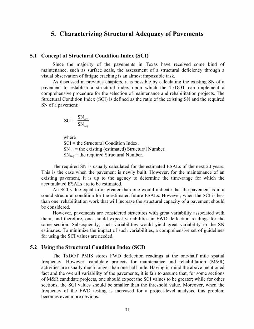
5.1 Concept of Structural Condition Index (SCI) Since the majority of the pavements in Texas have received some kind of
maintenance, such as surface seals, the assessment of a structural deficiency through a visual observation of fatigue cracking is an almost impossible task.
As discussed in previous chapters, it is possible by calculating the existing SN of a pavement to establish a structural index upon which the TxDOT can implement a comprehensive procedure for the selection of maintenance and rehabilitation projects. The Structural Condition Index (SCI) is defined as the ratio of the existing SN and the required SN of a pavement:
req
eff
SNSN
=SCI
where SCI = the Structural Condition Index. SNeff = the existing (estimated) Structural Number. SNreq = the required Structural Number.
The required SN is usually calculated for the estimated ESALs of the next 20 years. This is the case when the pavement is newly built. However, for the maintenance of an existing pavement, it is up to the agency to determine the time-range for which the accumulated ESALs are to be estimated.
An SCI value equal to or greater than one would indicate that the pavement is in a sound structural condition for the estimated future ESALs. However, when the SCI is less than one, rehabilitation work that will increase the structural capacity of a pavement should be considered.
However, pavements are considered structures with great variability associated with them; and therefore, one should expect variabilities in FWD deflection readings for the same section. Subsequently, such variabilities would yield great variability in the SN estimates. To minimize the impact of such variabilities, a comprehensive set of guidelines for using the SCI values are needed.
5.2 Using the Structural Condition Index (SCI) The TxDOT PMIS stores FWD deflection readings at the one-half mile spatial
frequency. However, candidate projects for maintenance and rehabilitation (M&R) activities are usually much longer than one-half mile. Having in mind the above mentioned fact and the overall variability of the pavements, it is fair to assume that, for some sections of M&R candidate projects, one should expect the SCI values to be greater; while for other sections, the SCI values should be smaller than the threshold value. Moreover, when the frequency of the FWD testing is increased for a project-level analysis, this problem becomes even more obvious.

32
Clearly using the average SCI value of the tested stations as the decision making criterion would not be suitable. This is due to the nature of the pavement variability. To address this problem, the researchers suggest using different and multiple criteria to define whether the project should be considered for M&R actions. For example, the use of two criteria would be more suitable. The first criterion is that at least 50 percent of stations where FWD testing is performed failed the SCI criterion to be greater than one. The second criterion would address the problem created when a selected M&R project is comprised of sections that are clearly in different structural conditions. For this case, researchers suggest the use of a threshold percentage (calibrated by the TxDOT) of tested stations whose SCI values are below the defined minimum SCI level. For example, if 20 percent or more of tested stations are below the minimum SCI value of 0.70, then the overall section is suitable for M&R activities.
Ultimately projects comprised of structurally different sections should be parceled into the sections that show similar structural conditions throughout the section. Selecting the particular type of rehabilitation work should follow the AASHTO Guide for Design of Pavement Structures for the calculated deficiency in the Structural Number (SN).
5.3 The Overall Condition of the TxDOT PMIS Sections For characterizing the overall condition of the TxDOT PMIS section, a total of
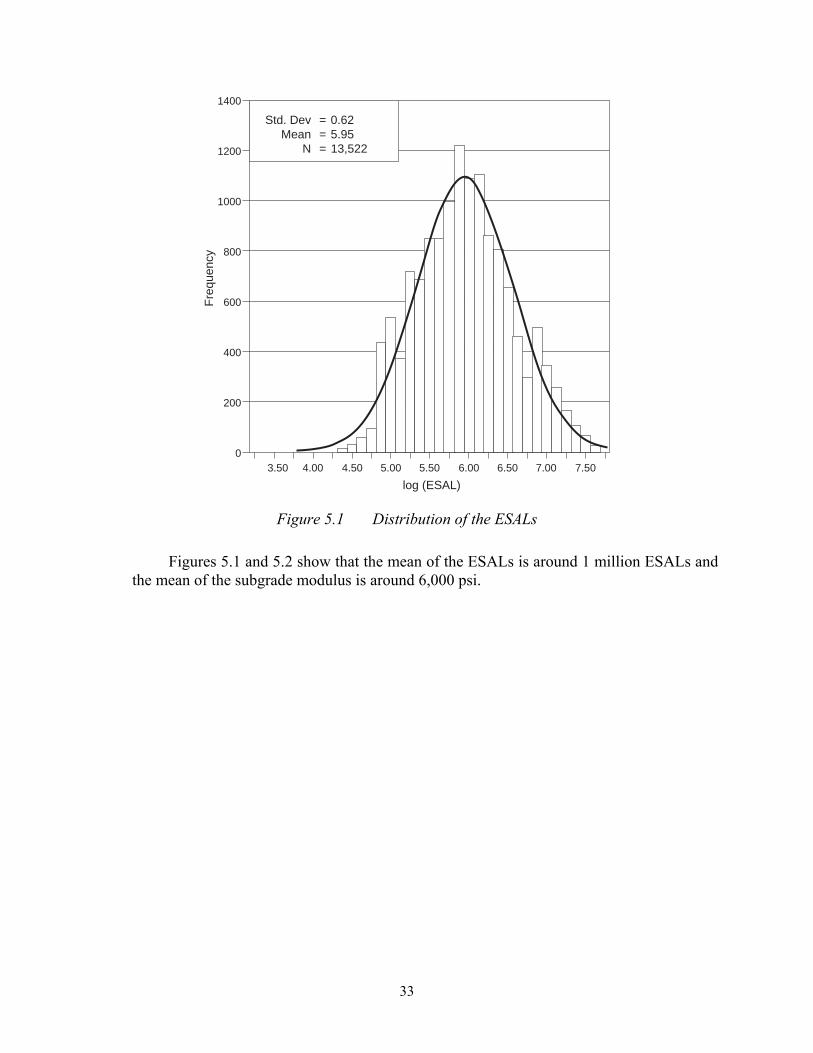
13,522 sections (of which, 7,460 sections were used for the validation analysis) were obtained from TxDOT PMIS. Those sections had different ESALs and subgrade modulus values. Figure 5.1 shows the distribution of the ESALs that have been normalized through a logarithmic transformation of the data; whereas Figure 5.2 shows a backcalculated subgrade modulus distribution that has been normalized by using the square root.
33
1400
1200
1000
800
600
400
200
03.50 4.00 4.50 5.00 5.50 6.00 6.50 7.00 7.50
log (ESAL)
Fre
quen
cy
Std. Dev = 0.62Mean = 5.95
N = 13,522
Figure 5.1 Distribution of the ESALs
Figures 5.1 and 5.2 show that the mean of the ESALs is around 1 million ESALs and the mean of the subgrade modulus is around 6,000 psi.

34
2000
1800
1600
1400
1200
1000
800
600
400
200
0
25 35 45 55 65 75 85 95 105 115 125 135
Square Root of Subgrade Modulus (Mr)
Fre
quen
cy
Std. Dev = 19.37Mean = 77.60
N = 13,522
Figure 5.2 Distribution of Squared Resilient Subgrade Modulus (Mr)
In order to portray the general structural condition of the pavements in the TxDOT PMIS, the SCI must be determined for each section. To do so, the required SN for the sections must be determined first. The required SN depends on the subgrade modulus and the 20-year accumulated ESALs. The subgrade modulus was divided into three categories and the 20-year accumulated ESALs, into five categories. Table 5.1 gives the values of the required SN for each category and it is calculated using design charts from the AASHTO Guide for Design of Pavement Structures 1993. The categories were represented with the average values. The limits of each Mr and 20-year accumulated ESAL level categories are set as preliminary values.

35
Table 5.1 Required SN for Different Categories of Accumulated ESAL Traffic and Mr.
20-Year Accumulated Traffic in ESALs Category Very Low Low Medium High Very High
Range 50,000 – 945,000
945,000 – 1,687,000
1,687,000 – 2,430,000
2,430,000 – 3,172,000
3,172,000 – 50,000,000
Category Range Average 498,000 1,316,000 2,059,000 2,801,000 26,586,000
Low 1,000 – 5,400 3,200 4.3 5.1 5.3 5.6 7.1
Medium 5,400 – 7,500 6,400 3.5 3.9 4.2 4.3 6.0
Mr (psi)
High 7,500 – 40,000 24,000 2.3 2.6 2.8 2.8 3.9
During the process of implementation the limits should be re-adjusted to conform
with the criteria TxDOT desires to set. For example, limits suggested by one of the project advisory members are as follows:
Table 5.2 Alternative Limits of the Mr and 20-Year Accumulated Traffic in ESALs
Mr (psi) Low: less than 8,000 Medium: 8,000 – 16,000 High: 16,000 and more
20-Year Accumulated Traffic in ESALs Very Low: less than 100,000 Low: 100,000 – 500,000 Medium: 500,000 – 3,000,000 High: 3,000,000 – 10,000,000 Very High: 10,000,000 and more
Having determined the required and effective SN using Method IV, one can easily
calculate the SCI values. The SCI distribution of the 7,460 sections from the TxDOT PMIS is presented in Figure 5.3. It can be observed that the average SCI for the assumed 20-year ESALs from the PMIS is 0.75.

36
1200
1000
800
600
400
200
00.2 0.4 0.6 0.8 1.0 1.2 1.4 1.6 1.8 2.0 2.2 2.4 2.6 2.8 3.0 3.2 3.4 More
Structural Condition Index (SCI)
Fre
quen
cyAverage: 0.75
Figure 5.3 Distribution of the Structural Condition Index

37
6. Determining FWD Testing Frequency at Network Level
6.1 Variability of Pavements Naturally, pavements inherit variabilities induced from various processes during the
construction. Even though the variability in pavement design was recognized in the early 1950s, the first analysis came with the AASHO Road Test (1956–1962). The conclusion was that even if the most rigorous control was put in place for every single process in highway construction, it would still be impossible to meet the specifications for many of the construction items [Carey 1966].
The most significant contributors to the pavement variability [Hughes 1996] are: a) Soil and aggregate material variability. b) Variability of asphalt concrete (AC) mix or Portland cement concrete (PCC). c) Variability of the construction process, like compaction or thickness consistency. d) Environmental conditions during the construction process. Recent studies have properly assessed pavement variabilities and have suggested
procedures for proper material specification and quality control of the construction process [Hughes 1996].
6.1.1 Structural Estimates of Pavements and Their Variability For the reasons stated in previous chapters, the SN estimates using Method IV were
chosen, and subsequently, the SCI is defined as the ratio of required to existing SN. Since the SCI is used as a screening tool to discriminate between pavements that need
structural reinforcement and those that do not, it is theoretically acceptable to use the variability of the SN as an indicator of pavement variability. Generally, the variability of the parameters computed from the deflection readings, such as a SN show greater variability than the initial deflection readings [Hossain 1992].
6.1.2 Propagation of the Variance The propagation of a variance of a multi-variable function can be portrayed using the
Taylor expansion. When a new random variable is introduced, the overall variance of a function increases. In the Method IV analysis, variance of FWD deflection readings is propagated to the SIP coefficient and, subsequently, to the SN estimate. Since the thickness is assumed to be uniform, variance of the SN depends only on the variance of the SIP coefficient. Naturally, the Structural Condition Index (SCI) variance is affected by the variance of existing SN. Under the assumption that the D(0) and D(1.5Hp) are independent, the following equations can be used to approximate propagation of the variance:
V [SIP] = V [D(0)] + V [D(1.5Hp)] V [SN] = (k1 * k2 * SIPk2-1*Hp
k3)2 * V [SIP]

38
V [SCI] = (1/SNreq) * V [SNeff]
Using the Structural Condition Index (SCI) as a screening tool for structural condition of the pavement at network level requires the establishment of confidence intervals. By doing so, the decision will not be influenced by the variability associated with the pavement structure. With that in mind, the agency’s interest was to set up the range of allowable or tolerable error for the SCI estimates. The allowable error will significantly influence the number of the sample size needed to satisfy a particular confidence interval.
Since the Structural Number (SN) varies from one pavement to another, depending on the structural condition of a pavement, normalized values of SNs should be used to set the allowable error. Therefore the allowable error should be set on the variance of SNs, in particular on the variance of the Coefficient of Variation (CV). For example, if one defines the allowable error to be 20 percent of the CV variance and the confidence level to be 80 percent and calculates the sample size, such sample size would insure that, with an 80 percent confidence level, the values of the SCI would be in the range of 20 percent from their true values.
6.1.3 Representing Pavement Variability at the Network Level The spatial distribution of the FWD data stored in the PMIS is based on tests
conducted with a frequency of one test for each half-mile section. However some half-mile sections contain deflection measurements with spacings of one-tenth of a mile. These sections allowed the researchers to conduct an in-depth assessment of the true variability associated with the pavements. It is understood that the variability also increases with age, but no data was available to characterize the impact of age on variability.
Sixty sections containing such data were selected and used in the analysis. Those sections are not uniform, but rather they represent pavements from different stages of their service life. In addition, those sections came from different functional categories of pavements. It is understood that the variability also increases with age, but no data was available to characterize the impact of age on variability.
As discussed briefly earlier, the sections considered were not adjacent to each other and the SN estimates for such sections were significantly different. Therefore, the Coefficient of Variation (CV) was used. The use of the CV has the advantage that the comparison of the variation can be conducted for different sections. The CV gives a relative variation that is normalized to the mean by expressing the standard deviation as a percentage of the mean.
6.2 Statistical Inferences It is a known statistical axiom that the accuracy for the estimated mean value of the
population increases with an increase in number of samples taken from the population. Therefore, standard error of sample means decreases by the square root of n, where n is a sample size. This represents the basis of the Central Limit Theorem.
There are many statistical methods for determining the sample size, such as the computer-intensive Bootstrap method, the Noether method and the risk-based method [Miller 1977]. The Bootstrap method is used in a situation where the form of the population is unknown, whereas the Noether method is more complicated and popular in

39
quantum physics. Among these methods, the risk-based method is the most effective and the one commonly adopted for engineering applications. The risk-based method produces the confidence intervals that imply that the mean of the population will be in a defined range.
The risk-based method considers two types of risks or errors. A type I error occurs whenever a product is rejected when it should have been accepted; whereas a type II error occurs whenever a product is accepted when it should be rejected. Therefore, there are two approaches for determining an adequate statistical sample size. One considers only the Type I error, and the other considers both the Type II and the Type I errors, with respect to the probabilities of erroneously rejecting or erroneously accepting a hypothesis. This is under the assumption that the distribution is gauss normal.
6.2.1 Controlling Only Type I Error Once the standard deviation is determined from the historical data, an engineer must
determine the desired level of confidence. The desired level of confidence is often expressed by probability in absolute terms, as
α−=≤− 1)|(| eyyP u
where y = sample mean.
uy = population mean. α = Type I error. e = tolerable error.
With the selection of a reasonable value for α (Type I error or producer’s risk) and e , which is called the margin of error or tolerable error, the required sample size can be determined by the following relationship:
2
22
2
e
Zn
σα
=
where n = sample size. Z 2α = the (1 − α / 2) percentile of the standard normal distribution.
σ = standard deviation. e = tolerable error.
6.2.2 Controlling Both Type I Error and Type II Error If it is the desire of the user to control both the Type I and Type II errors with the
selection of α (Type I error), β (Type II error), and a tolerable (allowable) error e, the required sample size can be determined using the following relationship:

40
2
22
2
e
ZZn
σβα
+
=
where n = sample size. α = Type I error. β = Type II error. Z
2α = (1 − α/2) percentile of the standard normal distribution.
βZ = the (1 − β ) percentile of the standard normal distribution. σ = standard deviation. e = tolerable (allowable) error.
In particular, when β = 0.5 (i.e., βZ = 0), the relationship would be identical to the one where only the Type I error is controlled.
6.3 Determining Sample Size It is a known fact that conducting more tests will yield more accurate results, but at
the same time, an increase in the number of tests will increase the cost of implementing such a procedure. In real life, economic constraints force engineers to keep the sample size as small as possible. Figure 6.1 shows the trade-off between the cost and failure rate from the perspective of testing frequency. Considering the vast highway network in Texas, it is very important that an appropriate testing frequency is used to balance between the level of confidence associated with maintenance decisions and the costs of conducting the tests.
Increasing Testing Frequency
Cos
ts D
ue to
Fai
lure
Failure Rate Costs
Test
ing
Cos
ts
Figure 6.1 The Trade-Off Between Testing Costs and Failure Rate

41
The AASHTO Guide for Design of Pavement Structures suggests limits in using accuracy curves for determining the sample size for a given confidence level and value of allowable error (R). The AAHSTO approach is identical to the approach presented above, when the Type I error is being controlled. In this study, instead of the letter R, the allowable or tolerable error is represented by the letter e. Given the circumstance that, in this case, the Type II error is very difficult to define, the analysis was conducted by considering only the Type I error. Having in mind the functional dependence of allowable error (R) and the required number of tests for the defined confidence interval, the allowable error was regionalized in three zones, shown in Figure 6.2.
n — Number of Tests/Measurements per Unit
±R V
alue
(U
nits
of P
aram
eter
)
Zone I
Zone II
Zone III
Figure 6.2 Typical Limit of Accuracy Curve for All Pavement Variables Showing General Zones [AASHTO 1993]
It can be observed that Zone I is characterized by the steep slope where the accuracy increases significantly with the number of tests, but yields a higher cost-benefit ratio. Zone III is a region with a relatively moderate slope where an increase in the number of samples will not result in a significant increase in accuracy. Zone II represents an optimal region for analysis, where the accuracy can be improved by a minimal increase in the number of tests [AASHTO 1993].
In the study conducted for the Kansas Department of Transportation (KDOT) [Hossain 1999], it was suggested that the “true” variation of the pavement could be obtained from deflection readings in increments of one-tenth of a mile. The analysis by Hossain suggested that for different control sections, the average allowable error was from 14 to 16 percent when the spatial test frequency was 3 tests per one mile. It also suggested that if the number of tests is increased to 5 tests per mile, the allowable error would be in range from 13 to 15 percent. An increase in FWD tests to 7 tests per mile would yield allowable error in the range from 12 to 13 percent. It is obvious that further increase in the number of tests will not yield a significant decrease in values of allowable error.

42
The Hossain assumption that “true” variability can be captured from the FWD tests with intervals of one-tenth of a mile is a fairly good assumption at network-level [Hossain 1999]. This holds for the nature of network-level analysis, where the interest is not in the specific pavement structures, but rather in the overall variability of the network.
Moreover, the sampling frequency of FWD tests at network level should not differentiate between the functional categories of the considered pavements, but rather the same policy should be adopted for the whole network. Considering the different construction procedures and quality control for different functional categories of the pavements in the highway network, one may overestimate the variability for pavements built with rigorous quality control. Such a phenomenon should not affect the procedure for determining the sample size, since the pavements with rigorous control come from the pavement category that is of higher importance to the network. Consequently, the confidence levels for such pavements would be higher−which is tolerable.
The mean values and the standard deviation of the existing SN were calculated for 60 different pavement sections in the PMIS. The length of the sections is one-half of a mile. As discussed above, different functional categories and conditions of pavements were represented in the sample. Coefficients of Variation (CV) were calculated for each section, and subsequently, the mean and the standard deviation of the CVs were obtained. Table 6.1 summarizes those results.

43
Table 6.1 Summary of Mean, Standard Deviations and Coefficients of Variances of the Existing SN for 60 Sections
Section Mean Standard Deviation CV (%) Section Mean Standard Deviation
CV (%)
1 7.45 0.61 8.24 31 1.60 0.71 44.55 2 4.73 0.94 19.97 32 1.43 0.27 19.02 3 0.86 0.01 1.28 33 1.59 0.36 22.61 4 8.28 0.52 6.30 34 1.35 0.24 17.85 5 4.57 1.20 26.27 35 1.84 0.48 25.91 6 7.29 1.14 15.63 36 2.21 0.70 31.71 7 5.38 2.20 40.79 37 2.12 0.69 32.74 8 3.95 2.34 59.29 38 1.68 0.08 4.83 9 4.84 0.83 17.22 39 2.05 0.59 28.76
10 5.82 1.45 24.93 40 1.58 0.11 7.13 11 3.43 0.88 25.80 41 1.44 0.26 18.07 12 3.36 0.80 23.88 42 1.35 0.10 7.59 13 3.73 1.03 27.65 43 1.49 0.46 31.07 14 1.14 0.05 4.31 44 1.44 0.27 18.92 15 2.14 0.73 34.33 45 1.66 0.24 14.21 16 2.48 0.36 14.57 46 2.54 2.28 89.76 17 2.93 0.25 8.65 47 1.00 0.08 8.16 18 2.80 0.39 14.03 48 1.09 0.10 8.78 19 2.91 0.24 8.29 49 1.05 0.04 3.86 20 2.92 0.25 8.56 50 1.02 0.03 3.00 21 2.60 0.43 16.48 51 1.10 0.07 6.06 22 2.60 0.88 33.84 52 1.03 0.05 4.56 23 1.96 0.76 38.71 53 1.12 0.05 4.28 24 2.13 1.01 47.75 54 1.01 0.05 4.94 25 1.61 0.23 14.00 55 0.93 0.05 5.81 26 1.60 0.09 5.57 56 0.96 0.06 5.84 27 2.78 1.47 53.00 57 0.97 0.07 6.73 28 1.57 0.19 12.26 58 0.92 0.05 5.95 29 1.77 0.51 29.02 59 1.07 0.14 13.30 30 1.55 0.97 62.69 60 1.00 0.09 9.20
Mean of CV = 20.14 %; Standard Deviation of CV = 17.29 %
6.4 Findings and Recommendations The information from Table 6.1 indicates that the mean and the standard deviation of
the CVs is 20 percent and 17 percent, respectively. However, for Sections 8, 27, 30 and 46, the relative variance is greater than 50 percent. It is interesting that for those sections some deflection readings indicated a very sound pavement, subsequently yielding very high values of existing SN. On the other hand, most of the other deflections indicated a poor structural condition. Basically, one deflection reading was very atypical for the section,

44
producing a large variance. Such an atypical deflection reading could be indicative of localized deep patching.
In a study conducted under the National Cooperative Highway Research Program’s (NCHRP) study [Hughes 1996], variabilities were classified by its source. The variabilities of soil, aggregate base, AC mix, and thickness were treated separately. The relative variability (CV) in pavement thickness from the NCHRP study corresponds to the values obtained under this study. Table 6.2 presents the CV values for different layers.
Table 6.2 Average Standard Deviation for Asphalt Concrete Pavement Thickness From New Jersey
Design Thickness (in) Average Thickness (in) Standard Deviation (in) CV (%) Surface, 1.5 1.73 0.26 15.0
Surface/Binder, 2.0 2.25 0.33 14.7 Surface/Binder, 3.0 3.37 0.42 12.5
Base, 4.0 4.00 0.56 14.0 Base, 6.0 5.99 0.56 9.3
6.4.1 Distribution of Coefficients of Variation (CV) The statistical inference and calculations of sample size were performed for two
cases. The assumption for the first case of the analysis is that the distribution of the CVs of the existing SN is normal. For the second case the assumption was that the CV of the existing SN is normally distributed if the data were transformed with the logarithm function. Figures 6.3 and 6.4 illustrate the histograms of the CVs for the 60 sections considered in the study. It can be observed that the distribution in Figure 6.4, after the data was transformed using logarithm function, is more similar to the normal gauss distribution than to the original distribution in Figure 6.3.

45
0
1
2
3
4
5
6
7
8
9
10
2 6 10 14 18 22 26 30 34 38 42 46 50 54 58 62 66 70 74 78 More
Coefficient of Variance
Freq
uenc
y
Figure 6.3 Histogram of the CV for 60 Sections Considered in the Analysis
0
1
2
3
4
5
6
7
8
0.1 0.3 0.5 0.7 0.9 1.1 1.3 1.5 1.7 1.9 2.1 2.3 2.5 2.7 2.9 More
Log (Coefficient of Variance (CV))
Freq
uenc
y
Figure 6.4 Histogram of the LOG CV for 60 Sections Considered in the Analysis

46
By setting different confidence levels and allowable error, one can estimate the approximate number of tests needed to satisfy those conditions. Table 6.3 summarizes those results. Table 6.3 shows that, by choosing the allowable error with a certain confidence level (1 − α/2), the agency can implement the sampling procedures. For example, if the agency defines the allowable error of the SN estimates to be 15 percent, and keeps the current sampling procedure, with one test per each half-mile section, the confidence level for such decisions is 80 percent.
Table 6.3 Number of Samples for Different Confidence Levels (CI) and Allowable Error (e) on Half-Mile Sections
NORMAL DISTRIBUTION Allowable Error (e)
Sample Size (n) 0.05 0.10 0.15 0.20 1 61 % 71 % 80 % 87 % 2 66 % 79 % 90 % 95 % 3 69 % 84 % 93 % 98 % 4 72 % 87 % 96 % 99 % 5 74 % 90 % 97 % ~100 %
LOG NORMAL DISTRIBUTION Allowable Error (e)
Sample Size (n) 0.05 0.10 0.15 0.20 1 55 % 60 % 65 % 70 % 2 57 % 64 % 71 % 77 % 3 59 % 67 % 75 % 82 % 4 60 % 70 % 78 % 85 % 5 61 % 72 % 81 % 88 %
This confidence level is considered to be low, even for the network-based decisions;
therefore, the agency should consider raising sampling frequency to two tests per half-mile section. This would produce a significant increase in the confidence level, from 80 to 90 percent.
If the distribution is being treated as a lognormal, the results will change, although the trends will remain the same. The same increase in the number of tests per half-mile section, from one test to two tests, will raise the confidence interval from 65 to 71 percent. If we consider the allowable error to be 20 percent, the confidence level would be increased from 70 to 77 percent.
It can be observed from Table 6.3 that the assumption on the distribution type highly affects the confidence intervals for the sample size. Further analysis in characterizing the type of the distribution of the SNs is therefore suggested.
Regardless of the type of the CV distribution, normal or lognormal, the results show an inadequate level of confidence for current M&R decision-making at the network level. It is recommended that the TxDOT increase the frequency of FWD tests to at least two tests per half-mile section.

47
7. Implementation of the Methodology
This chapter summarizes the equations and procedures needed to obtain the SCI. The developed methodology is fairly easy to implement, and the TxDOT PMIS stores all the information required for the implementation. The methodology consists of the following sequential steps:
1) Normalize measured FWD deflections to standard 9,000-lb load deflections.
2) Determine the deflection at an offset of 1.5 times the total pavement thickness (W1.5Hp). This requires interpolation among deflections measured at the fixed sensor positions. For this purpose, the following relationship can be used [Rohde 1994]:
DX = [(RX − RB)*(RX − RC)/(RA − RB)*(RA − RC)] * DA
+ [(RX − RA)*(RX − RC)/(RB − RA)*(RB − RC)] * DB
+ [(RX − RA)*(RX − RB)/(RC − RA)*(RC − RB)] * DC where DX = deflection at offset of RX. Di = deflection at sensor i. Ri = offset of Sensor i. i = A, B, C, the three closest sensors to Point X. X = point for which deflection is determined.
It should be noted that the above relationship is still valid even if the total thickness of a pavement is greater than 48 inches.
3) Determine the structural index of a pavement (SIP), using the following relationship:
SIP = W1 – W1.5Hp where SIP = structural index of pavement. W1 = peak deflection measured under a standard 9,000-lb FWD load (microns). W1.5Hp = surface deflection measured at offset of 1.5 times of Hp under a standard 9,000-lb FWD load (microns).
4) Determine the existing pavement structural number (SN) using the following relationship:
SNeff = k1 * SIPk2*Hp
k3 where

48
SNeff = existing pavement structural number (in). SIP = structural index of pavement (microns). Hp = total pavement thickness (mm). k1, k2, k3 = regression coefficients, listed in Table 7.1.
Since the information about the surface type of a pavement was not available in the PMIS, the researchers have assumed the asphalt concrete type of a surface, and consequently, the coefficients for that type should be used.
Table 7.1 Coefficients for Determining the SN
Surface Type k1 k2 k3 Surface Seals 0.1165 -0.3248 0.8241
Asphalt Concrete 0.4728 -0.4810 0.7581
5) Calculate the estimated subgrade resilient modulus (Mr): Mr = C*0.24*P/(W7*72) where Mr = backcalculated subgrade resilient modulus in psi. P = applied load in pounds. W7 = deflection at sensor 7 in inches. C = 0.33, as defined in the [AASHTO 1993].
6) For known values of the estimated subgrade resilient modulus (Mr) and the estimated future traffic in ESALs, determine the required SN using Table 7.2 that was developed according to the procedure discussed in Section 5.3. Of course, one could also use the SN equation from the AASHTO 1993 guides to calculate the required SN, even though it would make the implementation of the SCI procedure much more complicated.

49
Table 7.2 Required SN for Different Categories of Accumulated ESAL Traffic and Mr
20-Year Accumulated Traffic in ESALs Category Very Low Low Medium High Very High
Range 50,000 - 945,000
945,000 - 1,687,000
1,687,000 - 2,430,000
2,430,000 - 3,172,000
3,172,000 - 50,000,000
Category Range Average 498,000 1,316,000 2,059,000 2,801,000 26,586,000
Low 1,000 – 5,400 3,200 4.3 5.1 5.3 5.6 7.1
Medium 5,400 – 7,500 6,400 3.5 3.9 4.2 4.3 6.0
Mr (psi)
High 7,500 – 40, 000 24,000 2.3 2.6 2.8 2.8 3.9
7) For estimated values of the existing and the required SN, determine the Structural Condition Index (SCI) using the following relationship:
req
eff
SNSN=SCI
where SCI = the Structural Condition Index. SNeff = the existing (estimated) Structural Number. SNreq = the required Structural Number.


51
8. Pilot Project – Validation of the Procedure
8.1 Introduction Structural information on the three candidate projects scheduled for the rehabilitation
work was obtained from the Houston district. These projects are located on FM 762, FM 1463, and FM 1640. Each of those sections has experienced some fatigue (alligator) and longitudinal cracking. In order to assess the structural condition of the section, the SCI was calculated using the methodology developed under this study. The existing SN values were calculated using the Method IV described in previous chapters [Rohde 1994]. The advantage of this methodology is that it uses only total thickness and deflection readings as an input. Such information is available in the TxDOT Pavement Management Information System (PMIS). The required SN is estimated by using the methodology described in the AASHTO Guide for Design of Pavement Structures. The ESALs estimate for the calculation of the required SN was provided by the Houston district.
8.2 Overview of the Section’s Pavement Structure Generally, based on the information provided by the Houston district, the sections
considered have shown some fatigue (alligator) and longitudinal cracking. The results from the Ground Penetration Rader (GPR) testing have shown very few stripped areas in the bituminous layers.
Since FM 762 consists of different types of structural cross-sections, it was divided into four subsections that had a similar structure. Subsection 1 was defined from the intersection of FM 2759 SB for almost two miles. The surface and base layers constitute the total thickness of 13 - 14 inches. It is estimated that the subsection is characterized by 3 inches of Hot Mix Asphalt (HMA) over the 10-inch Asphalt Stabilized Base layer (ASB). The low-density layer at the bottom of the base is probably an old HMA layer (stripped or light-weight aggregate HMA). Subsection 2 was defined from Station 1 + 560 to 3 + 340 feet. It has the same structure as Subsection 1 (3 inches of HMA over 10 inches of base), but it does not have a thin layer at the bottom of the base layer. The base layer is possibly stabilized by asphalt cement, or it might have been treated by Portland cement (PC). Subsection 3 was defined from Station 3 + 340 to 10 + 370 feet. It is estimated for this subsection that the pavement structure has 6 - 8 inches of HMA over 10 - 12 inch base layer, with several full-depth HMA patches located between mileposts 8 and 9 offset from the start of the section. Subsection 4 was defined from Station 10 + 370 feet to the end of the section. It is estimated to have 3 - 4 inches of HMA over a 12-inch base layer. However, FWD deflection data was available only for the first 3 subsections and therefore, only these particular subsections were used in the analysis. In addition to this, the information provided by the Houston district suggests that this section has wet subgrade. In the analysis, the first two and the last two subsections were grouped, producing, for analysis purposes, subsections of 13 and 16 inches total thickness, respectively. The subsections of FM 762 are shown in the Figure 8.1.

52
3 inch
10 inch base(ASB)
3 inch
10 inch baseASB or CTB
6 inch HMA
10 inch base
3 inch HMA
10 inch base
IHp = 13"
0 + 000 1 + 560 3 + 340 10 + 370 15 + 388
IIHp = 13"
IIIHp = 16"
IVHp = 13"
Figure 8.1 The Pavement Structures of the Subsections for FM 762
The other two sections showed similar variability of the structural conditions and the total thickness. The total thickness of FM 1463 is estimated to be 13.5 inches, with 5.5 inches of asphalt concrete (AC) and an 8-inch base layer. In this analysis, the total thickness of FM 1640 is estimated to be 13 inches. The pavement structure of FM 1640 consisted of a 4-inch AC layer and a 9–inch flexible base layer.
Along with the available FWD deflection data, the total thickness of pavement information was used to calculate the existing SN using Method IV. Furthermore, the SCI values were calculated.
8.3 Section Analysis
8.3.1 Section FM 762 It was observed from an unpublished Memorandum provided by the Houston District
that FM 762 has alligator (fatigue) and longitudinal cracks, with a few spots where the stripping has occurred. The average SSI value for this section was 100. Figure 8.2 shows the calculated SCI values over the section station. In addition, distress score values of the section are shown above the SCI. The condition data for the section was also provided by the Houston district.

53
100
90
80
70
60
50
0 2 4 6 8 10 12
Station
Str
uctu
ral C
ondi
tion
Inde
x (S
CI) 2.0
1.5
1.0
0.5
0.0
Dis
tres
s S
core
Figure 8.2 The SCI and Distress Score Values for Section FM 762
It can be observed from the SCI - station graph that there are three distinct areas along the station. The first and the last subsections of the FM 762 section can be described as having a pavement structural condition that does not need any structural reconditioning, since the SCI values are well above the threshold value. The threshold value is indicated by the dashed line. On the other hand, the middle subsection (station from 2.5 to 7 mile post) does not have sufficient structural capacity based on the SCI values, and therefore needs structural reinforcement.
The FWD deflection data for the section FM 762 was also available to the researchers. The corresponding backcalculated moduli for each FWD test indicated a similar trend as the SCI. When the subsections are combined together as a project, it can be concluded that the section FM 762, as a whole section, needs reinforcement. In other words, the section is a good candidate for rehabilitation, which is consistent with the recommendation presented in the unpublished Memorandum that a 3-inch ACP overlay be applied to the section.
Figures 8.3 and 8.4 show the distribution and the cumulative distribution of the SCI for the section as a whole; whereas, Figures 8.5 and 8.6 show the distribution and the cumulative distribution for the middle subsection in the FM 762 section.

54
12
10
8
6
4
2
00.2 0.4 0.6 0.8 1.0 1.2 1.4 1.6 1.8 2.0
Structural Condition Index (SCI)
Fre
quen
cy
Figure 8.3 Distribution of the SCI Values for Section FM 762
100
80
60
40
20
00.2 0.4 0.6 0.8 1.0 1.2 1.4 1.6 1.8 2.0 More
Structural Condition Index (SCI)
Cum
ulat
ive
Per
cent
Figure 8.4 Cumulative Distribution of the SCI Values for Section FM 762

55
12
10
8
6
4
2
00.1 0.2 0.3 0.4 0.5 0.6 0.7 0.8 0.9 1.0 1.1 1.2 1.3 1.4 1.5 More
Structural Condition Index (SCI)
Fre
quen
cy
Figure 8.5 Distribution of the SCI Values for the FM 762 Middle Subsection
100
80
60
40
20
0
0.1 0.2 0.3 0.4 0.5 0.6 0.7 0.8 0.9 1.0 1.1 1.2 1.3 1.4 1.5 More
Structural Condition Index (SCI)
Cum
ulat
ive
Per
cent
Figure 8.6 Cumulative Distribution of the SCI Values for the FM 762 Middle Subsection
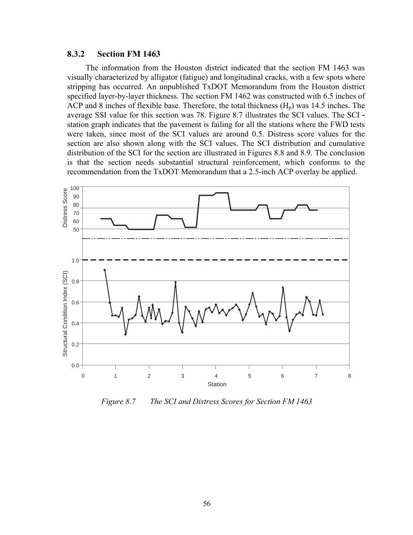
56
8.3.2 Section FM 1463 The information from the Houston district indicated that the section FM 1463 was
visually characterized by alligator (fatigue) and longitudinal cracks, with a few spots where stripping has occurred. An unpublished TxDOT Memorandum from the Houston district specified layer-by-layer thickness. The section FM 1462 was constructed with 6.5 inches of ACP and 8 inches of flexible base. Therefore, the total thickness (Hp) was 14.5 inches. The average SSI value for this section was 78. Figure 8.7 illustrates the SCI values. The SCI - station graph indicates that the pavement is failing for all the stations where the FWD tests were taken, since most of the SCI values are around 0.5. Distress score values for the section are also shown along with the SCI values. The SCI distribution and cumulative distribution of the SCI for the section are illustrated in Figures 8.8 and 8.9. The conclusion is that the section needs substantial structural reinforcement, which conforms to the recommendation from the TxDOT Memorandum that a 2.5-inch ACP overlay be applied.
100
90
80
70
60
50
0 1 2 3 4 5 6 7 8
Station
Str
uctu
ral C
ondi
tion
Inde
x (S
CI)
1.0
0.8
0.6
0.4
0.2
0.0
Dis
tres
s S
core
Figure 8.7 The SCI and Distress Scores for Section FM 1463

57
35
30
25
20
15
10
5
00.2 0.4 0.6 0.8 1.0 1.2 1.4 1.6 1.8 2.0
Structural Condition Index (SCI)
Fre
quen
cy
Figure 8.8 Distribution of the SCI Values for Section FM 1463
100
80
60
40
20
00.1 0.2 0.3 0.4 0.5 0.6 0.7 0.8 0.9 1.0 1.1 1.2 1.3 1.4 1.5
Structural Condition Index (SCI)
Cum
ulat
ive
Per
cent
Figure 8.9 Cumulative Distribution of the SCI Values for Section FM 1463

58
8.3.3 Section FM 1640 Like the other two sections, the information obtained from the Houston district
indicates that FM 1640 has visible distress, such as alligator and longitudinal cracking. The layer-by-layer thickness is: 4 inches of ACP 9 inches of flexible base, and 6 inches of stabilized subgrade. The stabilized subgrade was not considered in the total thickness. The average SSI value for this section was 86. As with the previous sections, the SCI values of FM 1640 vary for each station where the FWD deflection tests were performed. Figure 8.10 shows the SCI - station graph. It can be observed from the figure that the beginning of the section is characterized by large variability of the SCI values. Values of the SCI are in the range from 3.5 to 0.9. For the remaining stations, the SCI values did not exhibit such variability. The last two miles of the section indicate that the SCI values are solidly below the threshold value. The threshold value is represented by the dashed line. The general conclusion for this section is that it needs structural reinforcement. The results from the analysis conducted by the Houston district suggested 1.5-inch ACP overlay as the rehabilitation strategy. Figures 8.11 and 8.12 illustrate the SCI distribution and the cumulative distribution of the SCI values for the section.
807060504030
0.0 0.5 1.0 1.5 2.0 2.5 3.0 3.5 4.0
Station
Str
uctu
ral C
ondi
tion
Inde
x (S
CI)
3.5
3.0
2.5
2.0
1.5
1.0
0.5
0.0
Dis
tres
s S
core
Figure 8.10 The SCI and Distress Score Values for Section FM 1640

59
8
7
6
5
4
3
2
1
0
0.2 0.4 0.6 0.8 1.0 1.2 1.4 1.6 1.8 2.0 More
Structural Condition Index (SCI)
Fre
quen
cy
Figure 8.11 Distribution of the SCI Values for Section FM 1640
100
80
60
40
20
00.2 0.4 0.6 0.8 1.0 1.2 1.4 1.6 1.8 2.0 More
Structural Condition Index (SCI)
Cum
ulat
ive
Per
cent
Figure 8.12 Cumulative Distribution of SCI Values for Section FM 1463

60
8.4 Recommendations The evaluation of all three sections, using the developed SCI, shows that all sections
need some kind of structural reinforcement. The evaluations are consistent with the recommendations provided in Memorandums that were used as the information source in the analysis. The SCI shows different variability for each of the examined sections. To handle the variability, the researchers suggest the use of two criteria in the decision-making process. Such criteria were defined in Chapter 5. For the pilot project study, the researchers used the criteria that 50 percent of the stations were below the SCI threshold value of 1, and that the SCI values for more than 20 percent of the stations where the FWD tests were taken, were below 0.7. Under such criteria the examined sections were candidates for M&R. The specific type of M&R action should be selected for the average SN deficiency of the section.
Also, it is recommended that more sections from the TxDOT districts be used to further validate the SCI and corresponding procedures. In addition, the SSI values were calculated for each section and plotted together with the SCI values. The SSI values of the considered sections did not follow the trend of the distress score as the SCI did. Therefore, the SCI is a more reliable index to represent the structural capacity of a pavement section.

61
9. Conclusions and Recommendations
The objective of the project was to develop a methodology that could be used for discriminating between pavements requiring additional structural capacity and those for which surface treatments would be sufficient. This chapter presents the summary of the conclusions drawn from the research efforts and the recommendations for the use of the developed methodology.
9.1 Conclusions 1. A literature review of the potential methods for estimating structural condition
of pavements was undertaken. Different methods were evaluated. The key criterion for selecting a potential method was the availability of the data required by the potential method. The researchers have focused their attention on five different methods that have complied with such criterion. The output from these methods is either the estimated Structural Number (SN) of a pavement or the estimated moduli of the pavement layers.
2. Trend analyses were conducted to qualitatively characterize the proposed methods for evaluating the structural condition. The unit ESAL decrease (UED) of the PMIS condition scores was introduced as the variable for the sensitivity analysis. Such a variable has shown to be the best among all the considered deterioration descriptors. The methods considered showed different trends with respect to the UED. The best trends were established with Methods III and IV. Both of the methods give the estimated SN of a pavement as the result of the evaluation. The analysis was then undertaken to decide which method gave more accurate estimates, and which one was more suitable for the use in the PMIS. Since Method IV yielded better estimates of the SN than Method III, the researchers decided to use Method IV for the further development of the SCI. In addition, Method III requires the use of complicated regression-based formulas. The verification of the trends was conducted using the extended data set from the PMIS.
3. The Structural Condition Index (SCI) has been introduced as a screening tool to discriminate pavements that need structural reinforcement from those that do not. Furthermore, the guidelines for using such an index were developed. The SCI is defined as the ratio of the existing SN and the required SN of a pavement:
req
eff
SNSN
=SCI
where SCI = the Structural Condition Index. SNeff = the estimated existing Structural Number. SNreq = the required Structural Number.
62
4. A contingent sampling procedure was developed to determine the minimal
number of FWD tests required for each management section of pavements. Some half-mile sections stored in the PMIS contain FWD deflection measurements with spacings of one-tenth of a mile. These sections allowed the researchers to conduct an in-depth assessment of the variability associated with the pavements. Since the SN varies with the sections, the variability of the sections with respect to the SN was characterized by the Coefficient of Variation (CV) of the SN. Because of the variability of the SNs from one section to another, it has been concluded that the statistical inference for determining the sample size should be calculated using the mean and the standard deviation of the CVs. In addition, the researchers observed that, after the data were transformed using the logarithm function, the new distribution came to be closer to the normal gauss distribution than the original one. Regardless of the type of the CV distribution, normal or lognormal, the results show an inadequate level of confidence for current M&R decision-making at network level. It is recommended that the TxDOT increase the frequency of FWD tests to at least two tests per half-mile section.
9.2 Recommendations for Using the SCI Some recommendations for using the SCI are provided as follows:
1. The SCI index is sensitive to the UED pavement deterioration variables defined
in Chapter 3. The SCI should be used for each management section of the network. Clearly, using an average SCI value of the tested sections for the M&R project as the only criterion is not suitable, considering the general variability of the pavements. The researchers recommend the use of two criteria. The first criterion is that at least 50 percent of sections have a SCI value smaller than 1.0, and the second criterion is to use a threshold percentage (calibrated by the TxDOT) of sections tested with SCI values below the defined minimum SCI level. For example, if 20 percent or more of sections tested are below the minimum SCI value of 0.70, then the section as a whole should be budgeted for M&R activities. Also, it is recommended that such an M&R project be formed by aggregating sections that show similar structural conditions throughout the section.
2. Regardless of the type of the CV distribution, either normal or lognormal, the results show an inadequate level of confidence for the M&R decision-making at the network level. It is recommended that TxDOT increase the frequency of FWD tests to at least two tests per half-mile section.

63
References
[AASHTO 1993] AASHTO Guide for Design of Pavement Structures. AASHTO, Washington, DC, 1993.
[Carey 1966] Carey, W.N. Jr. and Shook, J.F., “The Need for Change in Construction Control Procedures,” Proceedings, National Conference on Statistical Quality Control Methodology in Highways and Airfield Construction, Charlottesville, VA, May 1966, pp 105-116.
[Hossain 1992] Hossain, M. and Zaniewski, J.P., “Variability in Estimation of Structural Capacity of Existing Pavements from Falling Weight Deflectometer Data,” Transportation Research Record 1355, TRB, Washington, DC, 1992, pp 17-26.
[Hosssain 1999] Hossain, M. and Chowdhury, T., “Use of Falling Weight Deflectometer Data for Assessing Pavement Structural Evaluation Values,” K-Tran KSU-96-4 Final Report, Kansas State University, Manhattan, KS, 1999.
[Hughes 1996] Hughes C.S., “Variability in Highway Pavement Construction,” NCHRP, Synthesis of Highway Practice 232, Washington, DC, 1996.
[Irwin 1983] Irwin, L.H., User’s Guide to Modcomp2, Version 2.1., Local Roads Program, Cornell University, Ithaca, NY, 1983.
[Miller 1977] Miller, I. and Freund, J.E., Probability and Statistics for Engineers, Prentice-Hall Inc., Englewood Cliffs, NJ, 1977.
[TxDOT 2000] Managing Texas Pavements, Texas Department of Transportation, Design Division, Pavements Section, November 2000.
[Rohde 1994] Rohde, G.T., “Determining Pavement Structural Number from FWD Testing,” Transportation Research Record 1448, Washington, DC, 1994.
[Romanoschi 1999] Romanoschi, S. and Metcalf, B., “Simple Approach to Estimation of Pavement Structural Condition,” Transportation Research Record 1652, Washington, D.C., 1999.
[Scullion 1988] Scullion, T., “Incorporating a Structural Strength Index into the Texas Pavement Evaluation System,” Research Report 409-3F, Texas Transportation Institute, Texas, April 1988.
[Wimsatt 1998] Wimsatt, A., “Improving the Texas Department of Transportation Pavement Rehabilitation Program,” Ph.D. Dissertation, The University of Texas at Austin, Austin, TX, May 1998.

64
[Wimsatt 1999] Wimsatt, A. “Direct Analysis Methods for Falling Weight Deflectometer Deflection Data,” Transportation Research Record, No. 1655, Washington, DC, 1999.

65
Appendix A

66

67
Figure A.1. Sensitivity of SN From Method III to the Yearly Change in Condition Score
Figure A.2. Sensitivity of SN from Method III to the Yearly Change in Normalized Condition Score
-4
-2
0
2
4
6
8
10
-80 -60 -40 -20 0 20 40 60 80 100 120
dCS
SN II
I
-4
-2
0
2
4
6
8
10
-6 -5 -4 -3 -2 -1 0 1 2
dCS/CS
SN II
I

68
Figure A.3. Sensitivity of SN From Method III to the UED of Condition Score
Figure A.4. Sensitivity of SN From Method IV to the Yearly Change in Condition Score
-4
-2
0
2
4
6
8
10
-500 -400 -300 -200 -100 0 100 200 300 400 500 600
UED (CS)
SN II
I
0
2
4
6
8
10
12
14
16
-80 -60 -40 -20 0 20 40 60 80 100 120
dCS
SN IV

69
Figure A.5. Sensitivity of SN From Method IV to the Yearly Change in Normalized Condition Score
Figure A.6. Sensitivity of SN From Method IV to the UED of Condition Score
0
2
4
6
8
10
12
14
16
-500 -400 -300 -200 -100 0 100 200 300 400 500 600
UED (CS)
SN IV
0
2
4
6
8
10
12
14
16
-6 -5 -4 -3 -2 -1 0 1 2
dCS/CS
SN IV

70
-500000
0
500000
1000000
1500000
2000000
2500000
3000000
3500000
-6 -5 -4 -3 -2 -1 0 1 2
dCS/CS
E p
Figure A.7. Sensitivity of Ep From Method II to the Yearly Change in Normalized
Condition Score
-500000
0
500000
1000000
1500000
2000000
2500000
3000000
3500000
-500 -400 -300 -200 -100 0 100 200 300 400 500 600
UED (CS)
E p
Figure A.8. Sensitivity of Ep From Method II to the UED of Condition Score

71
-4
-2
0
2
4
6
8
10
0 0.5 1 1.5 2 2.5 3 3.5
dRS
SN II
I
Figure A.9. Sensitivity of SN From Method III to the Yearly Change in Ride Score
-4
-2
0
2
4
6
8
10
0 0.1 0.2 0.3 0.4 0.5 0.6 0.7 0.8
dRS/RS
SN II
I
Figure A.10. Sensitivity of SN From Method III to the Yearly Change in Normalized Ride
Score

72
Figure A.11. Sensitivity of SN From Method III to the UED of Ride Score
Figure A.12. Sensitivity of SN From Method IV to the Yearly Change in Ride Score
-4
-2
0
2
4
6
8
10
0 10 20 30 40 50 60 70 80 90
UED (RS)
SN II
I
0
2
4
6
8
10
12
14
16
0 0.5 1 1.5 2 2.5 3 3.5
dRS
SN IV

73
0
2
4
6
8
10
12
14
16
0 0.1 0.2 0.3 0.4 0.5 0.6 0.7 0.8
dRS/RS
SN IV
Figure A.13. Sensitivity of SN From Method IV to the Yearly Change in Normalized Ride
Score
Figure A.14. Sensitivity of SN From Method IV to the UED of Ride Score
0
2
4
6
8
10
12
14
16
0 10 20 30 40 50 60 70 80 90
UED (RS)
SN IV

74
-500000
0
500000
1000000
1500000
2000000
2500000
3000000
3500000
0 0.1 0.2 0.3 0.4 0.5 0.6 0.7 0.8
dRS/RS
E p
Figure A.15. Sensitivity of Ep From Method II to the Yearly Change in Normalized Ride
Score
-500000
0
500000
1000000
1500000
2000000
2500000
3000000
3500000
0 10 20 30 40 50 60 70 80 90
UED (RS)
E p
Figure A.16. Sensitivity of Ep from Method II to the UED of Ride Score

75
-4
-2
0
2
4
6
8
10
0 10 20 30 40 50 60 70 80 90
UED (RS)
SN II
I T9T12T15
Figure A.17. Sensitivity of SN from Method III to the UED of Ride Score Stratified by
Thickness
0
2
4
6
8
10
12
14
16
0 10 20 30 40 50 60 70 80 90
UED (RS)
SN IV
T9T12T15
Figure A.18. Sensitivity of SN From Method IV to the UED of Ride Score Stratified by
Thickness

76
-4
-2
0
2
4
6
8
10
-500 -400 -300 -200 -100 0 100 200 300 400 500 600
dCS/(CS*Traffic)*10^6
SN II
I T9T12T15
Figure A.19. Sensitivity of SN From Method III to the UED of Condition Score Stratified
by Thickness
0
2
4
6
8
10
12
14
16
-500 -400 -300 -200 -100 0 100 200 300 400 500 600
dCS/(CS*Traffic)*10^6
SN IV
T9T12T15
Figure A.20. Sensitivity of SN From Method IV to the UED of Condition Score Stratified
by Thickness

77
-4
-2
0
2
4
6
8
10
12
14
16
0 10 20 30 40 50 60 70 80 90
UED (RS)
SN
SN IIISN IV
Figure A.20. Sensitivity of SNs From Methods III and IV to the UED of Ride Score
Figure A.21. Relationship Between Yearly Differences of Ride and Condition Score
-80
-60
-40
-20
0
20
40
60
80
100
120
0 0.5 1 1.5 2 2.5 3 3.5
dRS
dCS

78
0
20
40
60
80
100
120
-6 -5 -4 -3 -2 -1 0 1 2
dCS/CS
SSI
Figure A.22. Sensitivity of SSI to the Yearly Change in Normalized Condition Score
0
20
40
60
80
100
120
0 0.1 0.2 0.3 0.4 0.5 0.6 0.7 0.8
dRS/RS
SSI
Figure A.23. Sensitivity of SSI to the Yearly Change in Normalized Ride Score

79
Figure A.24. Sensitivity of SSI to the UED of Condition Score
Figure A.25. Sensitivity of SSI to the UED of Ride Score
0
20
40
60
80
100
120
-500 -400 -300 -200 -100 0 100 200 300 400 500 600
UED (CS)
SSI
0
20
40
60
80
100
120
0 10 20 30 40 50 60 70 80 90
UED (RS)
SSI

80

81
Appendix B

82

83
0
2
4
6
8
10
12
0 0.5 1 1.5 2 2.5 3 3.5 4 4.5
dRS
SN IV
Figure B.1. Sensitivity of SN From Method IV to the Yearly Change of Ride Score
0
2
4
6
8
10
12
0 20 40 60 80 100 120
dCS
SN IV
Figure B.2. Sensitivity of SN From Method IV to the Yearly Change of Condition Score

84
0
2
4
6
8
10
12
0 20 40 60 80 100 120
dDS
SN IV
Figure B.3. Sensitivity of SN From Method IV to the Yearly Change of Distress Score
Figure B.4. Sensitivity of SN From Method IV to the Yearly Change of Normalized Ride Score
0
2
4
6
8
10
12
0 0.1 0.2 0.3 0.4 0.5 0.6 0.7 0.8 0.9 1
dRS/RS
SN IV

85
0
2
4
6
8
10
12
0 0.2 0.4 0.6 0.8 1 1.2
dDS/DS
SN IV
Figure B.5. Sensitivity of SN From Method IV to the Yearly Change of Normalized Distress Score
Figure B.6. Sensitivity of SN From Method IV to the UED of Ride Score
0
2
4
6
8
10
12
0 20 40 60 80 100 120UED (RS)
SN IV

86
Figure B.7. Sensitivity of SN From Method IV to the UED of Condition Score
Figure B.8. Sensitivity of SN From Method IV to the UED of Distress Score
0
2
4
6
8
10
12
0 50 100 150 200 250 300
UED (DS)
SN IV
0
2
4
6
8
10
12
0 50 100 150 200 250 300
UED (CS)
SN IV

87
Figure B.9. Sensitivity of SN from Method IV to the UED of Ride Score, When Less Than 20
Figure B.10. Sensitivity of SN From Method IV to the UED of Ride Score, When dRS
Greater Than 0.2
0
2
4
6
8
10
12
0 5 10 15 20 25UED (RS)
SN IV
UED (RS) < 20
0
2
4
6
8
10
12
0 20 40 60 80 100 120 UED
SN IV
2635 data points: dRS>0.2

88
Figure B.11. Sensitivity of SN From Method IV to the UED of Ride Score, when dDS Greater Than 0 and dRS Greater Than 0.2
Figure B.12. Sensitivity of SN From Method IV to the UED of Distress Score, When dDS Greater Than 0 and dRS Greater Than 0.2
0
2
4
6
8
10
12
0 20 40 60 80 100 120
UED (RS)
SN IV
1311 data points:dDS>0 ; dRS>0.2
0
2
4
6
8
10
12
0 50 100 150 200 250 300
UED (DS)
SN IV
1311 data points:dDS>0 ; dRS>0.2