4-1

4. The Discrete Fourier Transform and Fast Fourier Transform

• Reference: Sections 8.0-8.7 of Text

Note that the text took a different point of view towards the derivation andthe interpretation of the discrete Fourier Transform (DFT). Our derivationis more “direct”.

• In many situations, we need to determine numerically the frequencyresponse of an analog system or the spectrum of an analog signal. Let ( )x tbe the signal under consideration. Then the procedure usually adopted is

1. Select a suitable sampling fequency 1/sf T= according to the Nyquistsampling criterion.

2. Sample ( )x t at time t nT= to obtain the discrete time (DT) signal [ ]x n .

3. If the discrete time signal is infinitely long, truncate it to a suitablelength, say N samples. Call the resultant signal ˆ[ ]x n .

4. Compute the Fourier transform (assuming a casual signal)

( )1

0

ˆ ˆ[ ]N

j j n

n

X e x n eω ω−

−

=

= ∑ (1)

at the desired frequencies. Note that if there is no need to truncate thesignal, then

( ) ( ) 1ˆ j jaX e X e X j

T Tω ω ω = =

4-2

where ( )aX jΩ is the Fourier transform of the analog signal ( )x t . Ingeneral,

( ) 1ˆ jaX e X j

T Tω ω ≈

• If the signal whose spectrum we want to deterime is a discrete time signal,then Steps 1 & 2 in the above procedure is no longer needed.

• This chapter is concerned with the efficient computation of Eqn (1) atdiscrete frequencies

2 / ; 0,1,..., 1k N k Nω π= = −

For convience, we will drop the sign ^ associated with ( )ˆ jX e ω and simply

use ( )jX e ω instead.

4.1 The Discrete Fourier Transfomr (DFT)

• The DFT of a finite duration (and casual) signal is defined as

( ) ( )1

2 /2 /

0

1

0

[ ] [ ]

[ ] ; 0,1,..., 1

Nj k N nj

k Nn

Nkn

Nn

X k X e x n e

x n W k N

πωω π

−−

==

−

=

= =

= = −

∑

∑

4-3

where2 /j N

NW e π−=

• In addition to being a sample of the FT at 2 /k Nω π= , the DFT coefficient[ ]X k also represents a sample of the ZT on the unit circle.

• The inverse discrete Fourier transform (IDFT) is

1

0

1[ ] [ ] ; 0,1,..., 1

Nkn

Nk

x n X k W n NN

−−

=

= = −∑

Proof:

1 1 1

0 0 0

1 1( )

0 0

1 1[ ] [ ]

1 [ ]

N N Nkn km kn

N N Nk k m

N Nk m n

Nm k

X k W x m W WN N

x m WN

− − −− −

= = =

− −−

= =

=

=

∑ ∑ ∑

∑ ∑

But

( ) (2 / )( )1( )

( ) (2 / )( )0

1 11 1

0

m n N j N m n NNk m n N

N m n j N m nk N

W eW

W e

N m n

m n

π

π

− − −−−

− − −=

− −= =− −

== ≠

∑

So

4-4

1

0

1[ ] [ ]

Nkn

Nk

X k W x nN

−−

=

=∑

• The DFT and the IDFT pair can also be represented in matrix form as

1 2 1

2 4 2( 1)

( 1) ( 1)2 ( 1)( 1)

1 1 1 1[0] [0]

1[1] [1]

1[2] [2]

1[ 1] [ 1]

NN N N

NN N N

N N N NN N N

X x

W W WX x

W W WX x

W W WX N x N

−

−

− − − −

= − −

LLL

M M M L MM ML

or=X Wx

where

1 2 1

2 4 2( 1)

( 1) ( 1)2 ( 1)( 1)

1 1 1 1[0] [0]

1[1] [1]

, , 1

[ 1] [ 1]1

NN N N

NN N N

N N N NN N N

x XW W W

x XW W W

x N X NW W W

−

−

− − − −

= = = − −

x X W

LLLM M M M M L ML

Note that

1 †1N

− =W W

where ( )†i denotes the Hermitian (or conjugate) transpose of a matrix.

4-5

• We can deduce from the matrix representation of the DFT that itscomputational complexity is in the order of ( )2O N .

• The Fast Fourier Transform (FFT) is an efficient algorithm for thecomputation of the DFT. It only has a complexity of ( )logO N N .

• From the DFT coefficients, we can compute the FT at any frequency.Specifically

( )1

0

1 1

0 0

1 1( 2 / )

0 0

( 2 / )1

( 2 / )0

[ ]

1 [ ]

1 [ ]

1 1 [ ]

1

1 [ ]

1

Nj j n

n

N Nkn j n

Nn k

N Nj k N n

k n

j k N NN

j k Nk

j N

X e x n e

X k W eN

X k eN

eX k

N e

e X k

N

ω ω

ω

ω π

ω π

ω π

ω

−−

=

− −− −

= =

− −− −

= =

− −−

− −=

−

=

= =

−=

−−

=−

∑

∑ ∑

∑ ∑

∑1

2 /0

N

j j k Nk e eω π

−

−=

∑

• Since the FT is the ZT evaluated on the unit circle, this means we can alsoobtain the ZT from the DFT coefficients by replacing the term je ω in theabove equation by z . In other word

4-6

( )1

1 2 /0

1 [ ]1

N N

j k Nk

z X kX z

N z e π

− −

−=

−=−∑

4.1.1 Convolution of Sequences

• Let 1[ ]x n and 2[ ]x n be two DT signals of duration N samples. We want toobtain their convolution:

1 2[ ] [ ] [ ]y n x n x n= ⊗

• Direct convolution leads to a complexity in the order of ( )2O N . With theavailability of the FFT, it is possible to perform the same task with acomplexity of only ( )logO N N .

The idea is to first multiply the DFT coefficients of the two signals togetherand then take an IDFT of the product.

This ideal, although simple, has to be exercised carefully.

• Let ( )1jX e ω , ( )2

jX e ω , and ( )jY e ω be the FTs of 1[ ]x n , 2[ ]x n , and [ ]y n

respectively. Then

( ) ( ) ( )1 2j j jY e X e X eω ω ω=

4-7

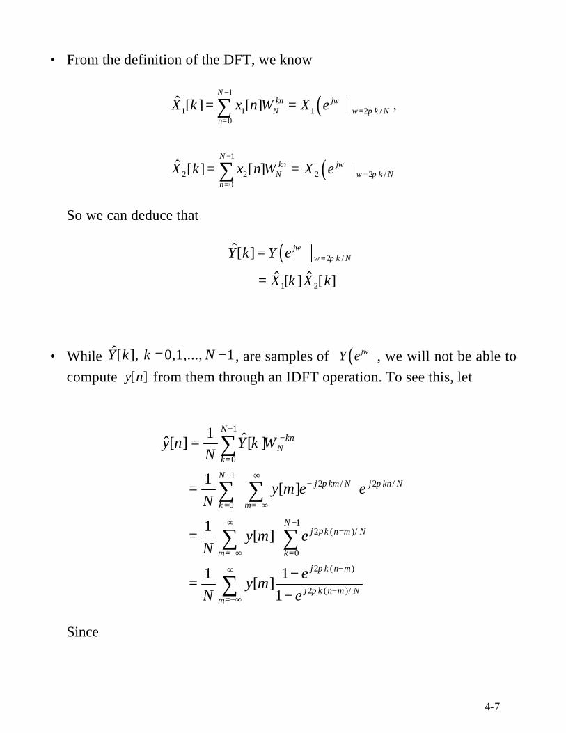
• From the definition of the DFT, we know

( )

( )

1

1 1 1 2 /0

1

2 2 2 2 /0

ˆ [ ] [ ] ,

ˆ [ ] [ ]

Nkn j

N k Nn

Nkn j

N k Nn

X k x n W X e

X k x n W X e

ωω π

ωω π

−

==

−

==

= =

= =

∑

∑

So we can deduce that

( ) 2 /

1 2

ˆ[ ]

ˆ ˆ [ ] [ ]

jk NY k Y e

X k X k

ωω π==

=

• While ˆ[ ], 0,1,..., 1Y k k N= − , are samples of ( )jY e ω , we will not be able tocompute [ ]y n from them through an IDFT operation. To see this, let

1

0

12 / 2 /

0

12 ( )/

0

2 ( )

2 ( )/

1 ˆˆ[ ] [ ]

1 [ ]

1 [ ]

1 1 [ ]

1

Nkn

Nk

Nj km N j kn N

k m

Nj k n m N

m k

j k n m

j k n m Nm

y n Y k WN

y m e eN

y m eN

ey m

N e

π π

π

π

π

−−

=

− ∞−

= =−∞

∞ −−

=−∞ =

−∞

−=−∞

=

= =

−=−

∑

∑ ∑

∑ ∑

∑

Since

4-8

2 ( )

2 ( ) /

10 otherwise1

j k n m

j k n m N

N m n rNe

e

π

π

−

−

= +− = − ,

the above becomes

ˆ[ ] [ ]r

y n y n rN∞

=−∞

= +∑

In other word, ˆ[ ]y n is an aliased version of [ ]y n .

• Example : Let

1 2

1 0 3[ ] [ ]

0 otherwise

nx n x n

≤ ≤= =

.

Then [ ]y n is a triangular signal

and ˆ[ ] 4y n = , n = 0,1,2,3.

1

3322

4

1n

0 1 2 3 4 5 6

4-9

• The cause for aliasing in ˆ[ ]y n is the lack of sufficient DFT coefficients inits construction. Note that [ ]y n is of duration 2 1N − samples so we need asmany DFT coefficients to capture all the information about the signal.

• To eliminate aliasing, we first treat 1[ ]x n and 2[ ]x n as signals with aduration of

2M N=

samples, where 1 2[ ] [ ] 0x n x n= = when 2 1N n N≤ ≤ − . Note that ingeneral, M can be any number as long as it is not smaller than the durationof [ ]y n .

We then take the M-point DFTs of 1[ ]x n and 2[ ]x n to obtain

( )

( )

1

1 1 1 /0

1

2 2 2 /0

[ ] [ ] ,

[ ] [ ] ,

Mnk j

M k Nn

Mnk j

M k Nn

X k x n W X e

X k x n W X e

ωω π

ωω π

−

==

−

==

= =

= =

∑

∑

After this, we form the product

( )1 2 /[ ] [ ] [ ] , 0,1,..., 1jk NY k X k X k Y e k Mω

ω π== = = −

Finally, we calculate the IDFT

4-10

1

0

1[ ] [ ] [ 2 ]

Mkn

Mk r r

Y k W y n rM y n rNN

− ∞ ∞−

= =−∞ =−∞

= + = +∑ ∑ ∑

Since the duration of [ ]y n is 2 1N − , which is less than M , the term[ 2 ]y n rN+ in the above equation equals to 0 for any 0r ≠ . Consequently

1

0

1[ ] [ ]

Mkn

Mk

Y k W y nN

−−

=

=∑

and there is no more aliasing.

4.1.2. Cicular Convolution and Aliasing

• We show in Section 4.1.1 that if we take the IDFT of the productcoefficients 1 2

ˆ ˆ ˆ[ ] [ ] [ ]Y k X k X k= , 0,1,..., 1k N= − , we obtain

ˆ[ ] [ ]r

y n y n rN∞

=−∞

= +∑ , (2)

which is an aliased version of [ ]y n .

• We will arrive at the same result through circular convolution of periodicsignals constructed from 1[ ]x n and 2[ ]x n .

4-11

• Let

( )1 1[ ]N

x n x n = %

and

( )2 2 [ ] ,N

x n x n = %

where ( )Nn is the modulo-N value of the integer n.

Because of the property of the modulo-N operation, the signals 1[ ]x n% and

2[ ]x n% are periodic with a period of N. Specifically,

1 1[ ] [ ], 0,1,..., 1x m rN x m m N+ = = −%and

2 2[ ] [ ], 0,1,..., 1x m rN x m m N+ = = −%

for any integer r .

• Conversely, the signals 1[ ]x n and 2[ ]x n can be obtained from 1[ ]x n% and

2[ ]x n% according to

1 1[ ] [ ] [ ]Nx n x n R n= %and

2 2[ ] [ ] [ ]Nx n x n R n= % ,where

1 0 1[ ]

0 otherwiseN

n NR n

≤ ≤ −=

4-12

is a rectangular windowing function.

• The circular or periodic convolution of 1[ ]x n% and 2[ ]x n% is defined as

1

3 1 20

[ ] [ ] [ ]N

m

x n x m x n m−

=

= −∑% % %

Clearly, 3[ ]x n% is a periodic signal with a period of N.

4-13

• We want to show that the signal ˆ[ ]y n in Eqn (2) is simply one period of

3[ ]x n% , i.e.

3ˆ[ ] [ ] [ ]Ny n x n R n= %

Proof:

- Since the signal 3[ ]x n% is periodic, we resctrict our attention to timeindices n between 0 and N-1.

- Since 0 1m N≤ ≤ − , the term 1[ ]x m% in the circular convolution is

simply 1[ ]x m .

- The index n m− of the term 2[ ]x n m−% can be as small as 1 N− or aslarge as 1N − . When 0n m− ≥ ,

2 2[ ] [ ]; 0x n m x n m n m− = − − ≥%

On the other hand when n m− is negative, then

2 2[ ] [ ]; 0x n m x N n m n m− = + − − <%

- The circular convolution can now be rewritten as:

1

3 1 20

1

1 2 1 20 1

1

1 2 1 20 1

[ ] [ ] [ ]

[ ] [ ] [ ] [ ]

[ ] [ ] [ ] [ ]

N

m

n N

m m n

n N

m m n

x n x m x n m

x m x n m x m x n m

x m x n m x m x N n m

−

=−

= = +−

= = +

= −

= − + −

= − + + −

∑

∑ ∑

∑ ∑

% % %

% % % %

4-14

1 1( )

1 20 0 0

1 1 1( )

1 21 0 0

1 1(

1 220 0

1 1ˆ ˆ [ ] [ ]

1 1ˆ ˆ [ ] [ ]

1 ˆ ˆ [ ] [ ]

n N Nkm r n m

N Nm k r

N N Nkm r N n m

N Nm n k r

N Nnr

N Nk r

X k W X r WN N

X k W X r WN N

X k X r W WN

− −− − −

= = =

− − −− − + −

= + = =

− −−

= =

=

+

=

∑ ∑ ∑

∑ ∑ ∑

∑∑ )

0

1 1 1( ) ( )

1 220 0 1

1 1 1( )

1 220 0 0

1 ˆ ˆ [ ] [ ]

1 ˆ ˆ [ ] [ ]

nr k m

m

N N Nn N r r k m

N Nk r m n

N N Nnr r k m

N Nk r m

X k X r W WN

X k X r W WN

−

=

− − −− + −

= = = +

− − −− −

= = =

+

=

∑

∑∑ ∑

∑∑ ∑

But

1( )

0

0 otherwise

Nr k m

Nm

N r kW

−−

=

==

∑

So

1

3 1 20

1 2

1 ˆ ˆ[ ] [ ] [ ]

ˆ ˆ IDFT [ ] [ ]

ˆ [ ]

Nnk

Nk

x n X k X k WN

X k X k

y n

−−

=

=

=

=

∑%

for 0 1n N≤ ≤ −

- We will discuss more about circular convolution in the section onOFDM modulation.

4-15

4.1.2 The DFT of an infinite-duration signal

• The DFT is defined only for a finite duration signal. As mentioned earlier,when the signal is of infinite duration, we must first truncate the signal to asuitable length before taking DFT. Truncation is equivalent to multiplyingthe infinitely long signal by the rectangular window function

1 0 1[ ]

0 otherwise

n Nw n

≤ ≤ −=

• Let [ ]x n and [ ] [ ] [ ]y n x n w n= be the signals before and after truncation. Asshown in Chapter 2, the FT of [ ]y n is

( ) ( ) ( )( )12

j j jY e X e W e dπ

ω θ ω θ

π

θπ

−

−

= ∫ ,

where ( )jX e ω and ( )jW e ω are respectively the FTs of the signal [ ]x n andthe windowing function [ ]w n .

• The DFT coefficients of the signal [ ]y n are

( )

1

0

1

0

2 /

[ ] [ ]

[ ]

; 0,1,..., 1

Nkn

Nn

Nkn

Nn

jk N

Y k y n W

x n W

Y e k Nωω π

−

=

−

=

=

=

=

= = −

∑

∑

4-16

• Since ( ) ( )j jY e X eω ω≠ , so the [ ]Y k s are not exactly the samples of

( )jX e ω at 2 /k Nω π= .

The spectral distortion can be reduced by using a longer truncation lengthand/or a different windowing function.

• Some commonly used windowing functions are

1. Hamming,2. Hanning,3. Kaiser, and4. Blackman

We will talk more about them in the Chapter on FIR filter design.

• Example : Let the original signal be

[ ] [ ]nx n a u n= .

where the parameter a is real, positive, and less than 1. The FT of thissignal is

( ) 11

j

jX e

aeω

ω−=−

Now, if we truncate this signal to N samples, we obtain the signal

[ ] 0 1[ ]

0 otherwisex n n N

y n≤ ≤ −

=

4-17

The DFT coefficients of this signal is

( )

( )

( ) ( )

1 1 12 /

0 0 0

2 /

2 /

2 /

2 /

[ ] [ ]

1

11

1 1

N N Nnkn n kn j k N

N Nn n n

Nj k N

j k N

N

j k N

N jk N

Y k y n W a W ae

ae

aea

ae

a X e

π

π

π

π

ωω π

− − −−

= = =

−

−

−

=

= = =

−=

−−=

−= −

∑ ∑ ∑

4.1.4 The DFT of a 2-sided signal

• In the definition of the DFT, the signal is implicitly assumed casual. In thiscase,

( )1

2 /0

[ ] [ ] ; 0,1,..., 1N

kn jN k N

n

X k x n W X e k Nωω π

−

==

= = = −∑

What happens when the signal is not casual, like the discrete-time versionof the SQRC pulse used in our project?

• Let [ ]x n be a non-casual signal time-limited to the range 2 2, 1N N− − ,where the duration N is assumed to be an even number.

One possible definition of the DFT of this signal is

4-18

[ ]

( )

1

20

12 /

20

12 ( /2 ) /

20

/ 2 12 /

/ 2

2 /

ˆ [ ]

NknN

Nn

Nj kn NN

n

Nj k n N N j kN

n

Nj km N j k

m N

j k jk N

X k x n W

x n e

x n e e

x m e e

e X e

π

π π

π π

π ωω π

−

=

−−

=

−− − −

=

−− −

=−

−=

= −

= −

= −

=

=

∑

∑

∑

∑.

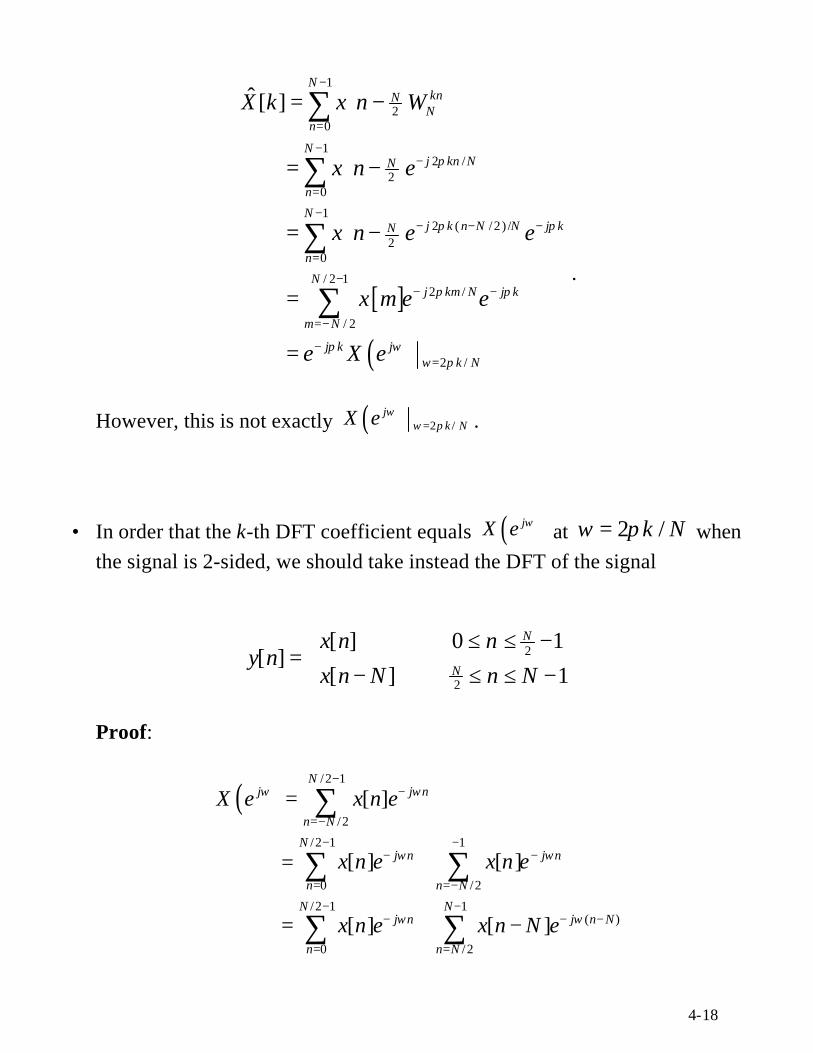
However, this is not exactly ( ) 2 /j

k NX e ωω π= .

• In order that the k-th DFT coefficient equals ( )jX e ω at 2 /k Nω π= whenthe signal is 2-sided, we should take instead the DFT of the signal

2

2

[ ] 0 1[ ]

[ ] 1

N

N

x n ny n

x n N n N

≤ ≤ −= − ≤ ≤ −

Proof:

( )/2 1

/2

/2 1 1

0 /2

/2 1 1( )

0 /2

[ ]

[ ] [ ]

[ ] [ ]

Nj j n

n N

Nj n j n

n n N

N Nj n j n N

n n N

X e x n e

x n e x n e

x n e x n N e

ω ω

ω ω

ω ω

−−

=−

− −− −

= =−

− −− − −

= =

=

= +

= + −

∑

∑ ∑

∑ ∑

4-19

Evaluating the above at 2 /k Nω π= yields

( )/ 2 1 1

2 / 2 ( )/2 /

0 /2

/ 2 1 1

0 / 2

1

0

[ ] [ ]

[ ] [ ]

[ ]

[ ]

N Nj j kn N j k n N N

k Nn n N

N Nkn kN

N Nn n N

Nkn

Nn

X e x n e x n N e

x n W x n N W

y n W

Y k

ω π πω π

− −− − −

== =

− −

= =−

=

= + −

= + −

=

=

∑ ∑

∑ ∑

∑

• In summary, for a 2-sided signal, we should first attach the negative-timeportion of the signal to the positive-time portion before taking DFT. Forexample, if the original signal is

then after manupulation, we have

4−n

2− 1− 0 1 2 33−

[ ]x n

n0 1 2 3 4 6 75

[ ]y n

4-20

4.2 The Decimation-in-Time FFT Algorithm

• Reference: Sections 9.1-9.3 of Text

• As discussed in the last section, the direct method of computing the DFTcoefficients has a complexity of 2N complex multiplications and ( )1N N −

complex additions.

Each complex multiplication itself requires 4 real multiplications and 2 realadditions.

Each complex addition involves two real additions.

So the total number of real multiplications is 24N and the total number ofreal addition is 24 2N N− .

• By decomposing the original N-point DFT into successively smaller DFTs(a divide-and-conquer approach), the amount of computations can bedramatically reduced. In this process, the properties of the complexexponential function

2 /j NNW e π−=

are exploited. Specifically, we notice that

1. ( )*( )k N n kn knN N NW W W− −= = (complex conjugate symmetry)

2. ( ) ( )kn k n N n k NN N NW W W+ += = (periodicity in n and k).

The resultant algorithms are collectively known as Fast Fourier Transform(FFT).

4-21

• We will focus in this section on the derivation of the decimation-in-timeFFT algorithm. For convenience, we assume

2vN =

where v is an integer. The idea, however, can be generalized to any othercomposite (i.e. non-prime) value of N .

• The DFT coefficients are given by

1

0

[ ] [ ] ; 0,1,..., 1N

knN

n

X k x n W k N−

=

= = −∑

Since 2vN = is an even number, we can express the above as the sum oftwo terms, one involving the even-numbered [ ]x n s, and the other involvingthe odd-numbered [ ]x n s:

even odd

/ 2 1 / 2 12 (2 1)

0 0

/ 2 1 / 2 12 2

0 0

[ ] [ ] [ ]

[2 ] [2 1]

[2 ] [2 1]

kn knN N

n n

N Nkr r k

N Nr r

N Nkr k kr

N N Nr r

X k x n W x n W

x r W x r W

x r W W x r W

− −+

= =

− −

= =

= +

= + +

= + +

∑ ∑

∑ ∑

∑ ∑

• The term 2krNW can be written as

2 2 (2 )/ 2 /( /2)/ 2

kr j kr N j kr N krN NW e e Wπ π− −= = =

4-22

Consequently [ ]X k can be rewritten as

/ 2 1 / 2 12 2

0 0

/ 2 1 / 2 1

/ 2 / 20 0

[ ] [2 ] [2 1]

[2 ] [2 1]

[ ] [ ]

N Nkr k kr

N N Nr r

N Nkr k kr

N N Nr r

X k x r W W x r W

x r W W x r W

G k H k

− −

= =

− −

= =

= + +

= + +

= +

∑ ∑

∑ ∑

where/ 2 1

/ 20

[ ] [2 ] ; 0,1,..., 1N

krN

r

G k x r W k N−

=

= = −∑and

/ 2 1

/ 20

[ ] [2 1] ; 0,1,..., 1N

krN

r

H k x r W k N−

=

= + = −∑

• Since

( /2)/ 2 / 2m N r mr

N NW W+ = ,

this means

[ /2] [ ]; 0,1,... / 2 1G m N G m m N+ = = −

and[ /2] [ ]; 0,1,... / 2 1H m N H m m N+ = = − .

Moreover, the [0], [1],..., [ / 2 1]G G G N − are the DFT coefficients of thesubsequence [2 ]x n . Similarly, [0], [1],..., [ / 2 1]H H H N − are the DFTcoefficients of the subsequence [2 1]x n + .

4-23

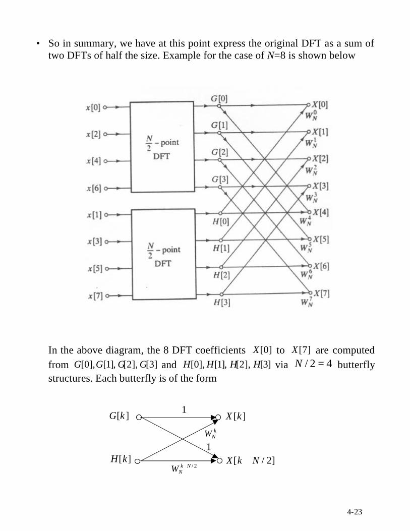
• So in summary, we have at this point express the original DFT as a sum oftwo DFTs of half the size. Example for the case of N=8 is shown below

In the above diagram, the 8 DFT coefficients [0]X to [7]X are computedfrom [0], [1], [2], [3]G G G G and [0], [1], [2], [3]H H H H via / 2 4N = butterflystructures. Each butterfly is of the form

/ 2k NNW +

kNW

1

1[ ]G k

[ / 2]X k N+

[ ]X k

[ ]H k

[ ]G k

4-24

• The butterfly used in the computation of the DFT is an example of a signalflow graph (essentially a computational structure).

In general, a signal flow graph would consist of a set of nodes or states (asrepresented by the circles in the butterfly structure) interconnected by a setof directed branches. The weights (as represented by the parameters 1, 1,

kNW , and / 2k N

NW + in the butterfly) associated with the branches are calledtransmittances. The transmittance from node j to node k might be denotedby jkt in general.

Associated with each node in the signal flow graph is a variable or nodevalue. The value associated with node k might be denoted by ks and isequal to

1

L

k j jkj

s s t=

= ∑

• The butterfly shown in the previous page requires 2 complexmultiplications and 2 complex additions. But since

/ 2k N kN NW W+ = − ,

the number of multiplications can be reduced to 1 if the following structureis adopted instead

1[ ]G k

kNW

1

1[ ]G k

[ / 2]X k N+

[ ]X k

[ ]H k

[ ]G k

1−

4-25

So in total, the complexity of the 4 butterflies in the above example is 4complex multiplications (CM) and 8 complex additions (CA). In general,there are / 2N CMs and N CAs.

• Since 2vN = , / 2N is also an even number. This means each of the two/ 2N -point DFT in the above example can be expressed in terms of two/ 4N -DFTs. For example, we show below the computation of

[0], [1], [2], [3]G G G G from [0], [2], [4], [6]x x x x .

The overall computational structure now takes on the form shown in thediagram in the next page. The two / 2N -point DFTs are now replaced by 4butterflies.

Since the number of butterflies in the second stage (from the right) is thesame as that in the first stage, the computational complexities of bothstages are identical and equal to 4 CMs and 8 CAs.

In general, (when 2vN = ,) there are always / 2N butterflies at each stage.

4-26

• Each of the four / 4N -point DFTs in the above example can be computedusing the following butterfly

Notice that there is actually no need to perform any multiplication. Forsimplicity though, we assume the complexity of this butterfly is the same asthe one that we presented earlier, i.e. 1 CM and 2 CAs.

1

02 1W =

1 / 22 1N

NW W= = −

1[ ]G k

4-27

• It is evident that when 2vN = , there will be altogether v stages in theoverall computational structure, with / 2N butterflies at each stage.

4-28

The total number of complex multiplications is thus

2

11 log ( )

2 2M

Nn v N N= × × =

The total number of additions is

22 log ( )A Mn n N N= = .

In conclusion, the complexity of this decimation-in-time algorithm is in theorder of logN N , which is much smaller than 2N for large N.

• It is observed from the 8N = example that the input data needed to beshuffled before being any computation can be take place. This can be donethrough the bit-reversal algorithm.

Let

( )[0], [1],..., [ ],..., [ 1]a a a n a N= −A

be the array containing the shuffled data. In the 8N = example, this vectoris ( )[0], [4], [2], [6], [1], [5], [3], [7]x x x x x x x x=A . Furthermore, let

( )1 2 0, ,..., ; 0,1v v jb b b b− −= ∈B

be the natural binary representation of the integer n , i.e.

1

0

2v

jj

j

n b−

=

= ∑Then

[ ] [ ]a n x m=

4-29

where1

1

0

2v

v jj

j

m b−

− −

=

= ∑

is the decimal equivalent of the binary vector

( )0 1 1, ,...,r vb b b −=B .

• Exercise: Show that if [ ] [ ]a n x m= , then [ ] [ ]a m x n= , i.e. the samples arepair-wise interchanged.

• In-place computations

The FFT algorithm computes the DFT coefficients in stages.The input data at the (m-1)-th stage ( 0 to m v= from left to right) aretransformed into another set of data that will be used in the computations inthe m-th stage.

Clearly, we can store the data to be computed in one array and those usedin the computation in another array. This requires a total of 2N storage.

However, the FFT algorithm we just described can be used to implementin-place computations. This will essentially reduce the storage to about50%.

Let us first index the data at the m-th stage in the signal flow graph as[ ]mX l , where 0,1,..., 1N= −l (from top to bottom), then it can be easily

shown that the pair

( )[ ], [ ]m mX p X q

4-30

can be computed exclusively from the pair

( )1 1[ ], [ ]m mX p X q− −

using the butterfly

This means as far as data storage is concerned, we need only one array ofN samples (and a temporary buffer of 2 samples). At the beginning of them-th stage, this array stores all the 1[ ]mX − l , 0,1,..., 1N= −l . As soon as

[ ]mX p and [ ]mX q are computed, the corresponding entries in the array arethen updated.

• There are other versions of FFT that do not require re-ordering of the input;see Fig. 9.14-9.16 of Text. Some of these algorithms, however, have thedisadvantage that computations can not be implemented in place. Others,on the other hand, requires re-ordering of the output (see for example thedecimation-in-frequency FFT algorithm described in Section 9-4).

• Algorithms for general value of N may have more complicated indexingproblem.

1[ ]mX q−

1[ ]G k

rNW

1

1[ ]G k1[ ]mX p−

1−

[ ]mX p

[ ]mX q

4-31

4.3 Application of FFT in OFDM

• References:

1. Chapter 12 of the book by J. G. Proakis, Digital Communicaitons,McGraw Hill, 4th Edition, 2001.

2. IEEE Standard 802.11a-1999, Part 11: Wireless LAN Medium AccessControl (MAC) and Physical Layer (PHY) Specifications – High SpeedPhysical Layer in the 5 GHz Band.

3. ADSL Tutorial at

http://www.rad.com/networks/1997/adsl/AdslMainPage.htm

• Orthogonal Frequency Division Multiplexing (OFDM) is a parallelmodulation format. Instead of transmitting data serially at a high speedwith a single carrier, an OFDM modem organizes the data into N lower-rate substreams and transmit the data in the different substreams at differentcarrier frequencies.

Conventional serial modem

High rate data

cf

QAM Modulator ( )z t%Bit duration

4-32

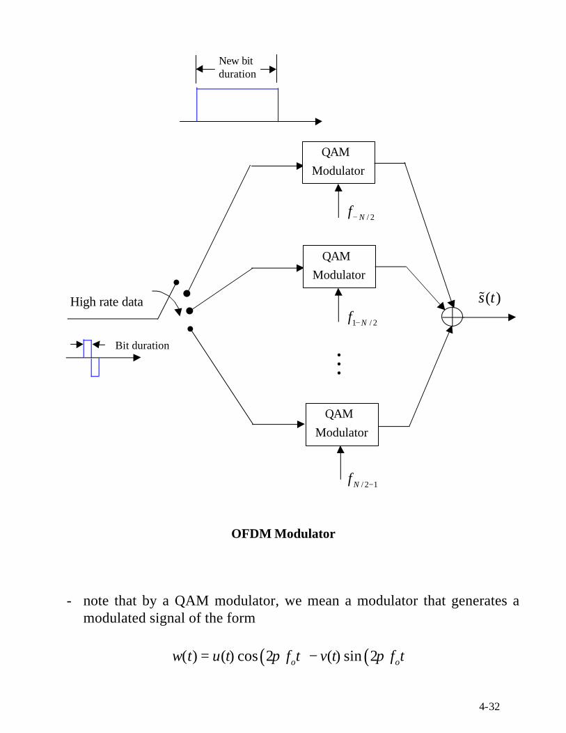
OFDM Modulator

- note that by a QAM modulator, we mean a modulator that generates amodulated signal of the form

( ) ( )( ) ( ) cos 2 ( ) sin 2o ow t u t f t v t f tπ π= −

New bitduration

High rate data ( )s t%

Bit duration

/ 2 1Nf −

1 / 2Nf −

/ 2Nf−

QAM

Modulator

QAM

Modulator

QAM

Modulator

M

4-33

from the input data. Here ( )u t and ( )v t are baseband pulse-amplitudemodulated (PAM) signals. Example of a QAM modulator is QPSK.

- Spectral characteristics of conventional serial modulation and OFDM

Spectral characteristics of conventional serial modem. sT is thesymbol duration of the signal ( )z t% .

Spectral characteristics of the OFDM signal ( )s t% . T is the symbolduration in the subchannels and 1/ aT is the frequency separationbetween adjacent subchannels.

cff

1/ sT

1/T

1/ aT

••••

f

cf

4-34

• Why OFDM?

In many applications, the communication channel is not ideal, i.e. itsfrequency response is not flat (nor linear phase) over the transmission band.

A nonideal channel causes severe intersymbol interference (ISI) in serialmodems.

By dividing the entire transmission band into subchannels, then as long asthe frequency response over a subchannel is flat (and linear phase), thatsubchannel is ideal.

• The subchannel spacing (and the number of subchannels) is thus a functionof the coherent bandwidth of the channel.

4.3.1 The Basic OFDM Signal Structure

• Data in an OFDM system is organized into frames. In the basic OFDMsystem, each frame is of duration aT sec, where 1/ aT is the symbol rate ofeach subchannel.

• Without loss in generality, we can focus on the frame in the interval [0, ]aT .The OFDM signal in this interval can be written as

/ 2 1

/ 2

1( ) ( ); 0

N

k ak N

s t s t t TN

−

=−

= ≤ ≤∑% %

where

4-35

( ) ( )( ) [ ]cos 2 [ ]sin 2k k ks t X k f t Y k f tπ π= −%

is the output signal of the k-th QAM modulator. In the above equation,

[ ] 1, 3, , ( 1)X k Q∈ ± ± ± −…and

[ ] 1, 3, , ( 1)Y k Q∈ ± ± ± −…

are respectively the in-phase (I) and quadrature (Q) channel data of the k-th modulator in the interval [0, ]aT ,

2M Q=

is the number of points in the signal constellation, and

k c

a

kf f

T= +

is the k-th subcarrier frequency. The term cf is the center frequency of theOFDM signal.

• The signal constellation of the k-th modulator is obtained by plotting allpossible

[ ] [ ] [ ]S k X k jY k= +

as points in the complex plane; see the examples below.

It is possible to use different constellations in different subchannels. A“good” subchannel can use a denser (and hence more efficient)constellation while a “bad” channel uses a less dense constellation.

4-36

Signal constellations of BPSK, QPSK, 16QAM and 64QAM. The binarypatterns in these constellations are the information contained in thesignal points.

4-37

• Exercise: Show that the overall bit rate of the above OFDM signal is

2

1logb

a

R N MT

= × ×

• Exercise: Convince yourself that when Q=2, the signal in each subchannelis a QPSK signal with rectangular pulse shaping.

• Consider the pairwise correlation of the subchannel signals:

( ) ( )

( ) ( )

( ) ( )

0 0

0

0

( ) ( ) [ ]cos 2 [ ]sin 2

[ ]cos 2 [ ]sin 2

[ ] [ ]cos 2 cos 2

[ ] [ ]si

a a

a

a

T T

k m k k

m m

T

k m

T

s t s t dt X k f t Y k f t

X m f t Y m f t dt

X k X m f t f t dt

Y k Y m

π π

π π

π π

= −

−

=

+

∫ ∫

∫

∫

% %

( ) ( )

( ) ( )

( ) ( )

0

0

n 2 sin 2

[ ] [ ]cos 2 sin 2

[ ] [ ]sin 2 cos 2

a

a

k m

T

k m

T

k m

f t f t dt

X k Y m f t f t dt

Y k X m f t f t dt

π π

π π

π π

−

−

∫

∫

Since

4-38

( ) ( ) ( ) ( )

( ) ( ) 0 0

0

1cos 2 cos 2 cos 2 [ ] cos 2 [ ]

2

1 cos 4 2 cos 2

2

/ 2

a a

a

a a

T T

k m k m k m

T

k m k mc T T

a

f t f t dt f f t f f t dt

f t t t dt

T

π π π π

π π π+ −

= + + −

= + +

=

∫ ∫

∫

,0

k m

k m

=

≠

( ) ( ) ( ) ( )

( ) ( ) 0 0

0

1sin 2 sin 2 cos 2 [ ] cos 2 [ ]

2

1 cos 2 cos 4 2

2

/ 2

a a

a

a a

T T

k m k m k m

T

k m k mcT T

a

f t f t dt f f t f f t dt

t f t t dt

T

π π π π

π π π− +

= − − +

= − +

=

∫ ∫

∫

,0

k m

k m

=

≠

and

( ) ( ) ( ) ( )

( ) ( ) 0 0

0

1sin 2 cos 2 sin 2 [ ] sin 2 [ ]

2

1 sin 2 sin 4 2

2

0

a a

a

a a

T T

k m k m k m

T

k m k mcT T

f t f t dt f f t f f t dt

t f t t dt

π π π π

π π π− +

= − + +

= + +

=

∫ ∫

∫

when 1/c af T>> , the correlation becomes

( )2 2

0

[ ] [ ] / 2 ( ) ( )

0

aTa

k m

X k Y k T k ms t s t dt

k m

+ == ≠

∫ % % .

In other word, the signals in different subchannels are orthogonal to oneanother and hence the term OFDM.

4-39

• To ensure orthogonality, the different QAM modulators must be in phase-synchronsim. This is because

( ) ( )

( ) ( ) 0

[ ]cos 2 [ ]sin 2

[ ]cos 2 [ ]sin 2 0

aT

k k k k

m m m m

X k f t Y k f t

X m f t Y m f t dt

π φ π φ

π φ π φ

+ − + ×

+ − + ≠

∫

if the phases kφ and mφ are different. Unfortunately, it will be verycomplicated and expensive to keep the different modulators in phase-syncusing analog technologies.

A DSP approach, based on FFT, can get around the problem.

• Consider the k-th subchannel signal again. This signal can be written as

( ) ( )( ) ( )

( ) ( ) ( ) ( )

( ) [ ]cos 2 [ ]sin 2

Re [ ] [ ] cos(2 ) sin(2 )

Re [ ]exp 2

Re [ ]exp 2 exp 2

Re ( )exp 2

a

k k k

k k

k

kcT

k c

s t X k f t Y k f t

X k jY k f t j f t

S k j f t

S k j t j f t

s t j f t

π π

π π

π

π π

π

= −

= + +

=

=

=

%

where

( ) [ ]exp 2ka

ks t S k j t

Tπ

=

is the baseband equivalent (or complex envelop) of ( )ks t% .

4-40

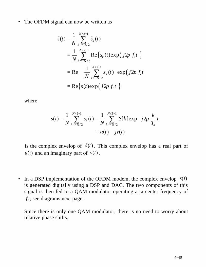
• The OFDM signal can now be written as

( )

( )

( )

/ 2 1

/ 2

/ 2 1

/ 2

/ 2 1

/ 2

1( ) ( )

1 Re ( )exp 2

1 Re ( ) exp 2

Re ( )exp 2

N

kk N

N

k ck N

N

k ck N

c

s t s tN

s t j f tN

s t j f tN

s t j f t

π

π

π

−

=−

−

=−

−

=−

=

=

= =

∑

∑

∑

% %

where

/ 2 1 /2 1

/ 2 /2

1 1( ) ( ) [ ]exp 2

( ) ( )

N N

kk N k N a

ks t s t S k j t

N N T

u t jv t

π− −

=− =−

= =

= +

∑ ∑

is the complex envelop of ( )s t% . This complex envelop has a real part of( )u t and an imaginary part of ( )v t .

• In a DSP implementation of the OFDM modem, the complex envelop ( )s tis generated digitally using a DSP and DAC. The two components of thissignal is then fed to a QAM modulator operating at a center frequency of

cf ; see diagrams next page.

Since there is only one QAM modulator, there is no need to worry aboutrelative phase shifts.

4-41

Baseband segment of the OFDM modulator

IF/RF segment of OFDM modulator

• Let

/[ ] ( )at nT Ns n s t ==

be the DT signal obtained by sampling the baseband OFDM signal ( )s t attime / ; 0,1,..., 1at nT N n N= = − . This means

( )v t

( )u t

[ ]v n

[ ]u n

[ ]/ 2 1S N− +

[ ]1s N −

[ ]1s

[ ]0s

[ ]/ 2S N

[ ]/ 2S N−

IFFT

[ ]Re •

[ ]Im •

DAC

DAC

M M

( )s t%

( )v t

( )u t

cos(2 )cf tπ

sin(2 )cf tπ−

4-42

/ 2 1

/ 2 /

/ 2 1

/ 2

/ 2 1

/ 2

/ 2 1 1

0 / 2

/ 2 1

0

1[ ] [ ]exp 2

1 [ ]exp 2

1 [ ]

1 1 [ ] [ ]

1 [ ]

a

N

k N a t nT N

Na

k N a

Nkn

Nk N

Nkn kn

N Nk k N

Nkn

Nk

ks n S k j t

N T

nTkS k j

N T N

S k WN

S k W S k WN N

S k WN

π

π

−

=− =

−

=−

−−

=−

− −− −

= =−

−−

=

=

=

=

= +

=

∑

∑

∑

∑ ∑1

( )

/ 2

/ 2 1 1

0 / 2

1

0

IDFT of [ ]

1 [ ]

1 1 [ ] [ ]

1 [ ] ; 0,1,2,..., 1

Nk N n

Nk N

N Nkn kn

N Nk k N

Nkn

Nk

D k

S k N WN

S k W S k N WN N

D k W n NN

−− −

=

− −− −

= =

−−

=

+ −

= + −

= = −

∑ ∑

∑ ∑

∑1442443

where

[ ] 0,1,..., / 2 1[ ]

[ ] / 2,..., 1

S k k ND k

S k N k N N

= −= − = −

represents the permutated data in the different subchannels.

At this point, it is obvious that we can exploit the efficiency of the FFT tocompute the [ ]s n ’s.

The signal ( )s t is obtained by passing the [ ]s n ’s to a digital to analogconverter (DAC).

4-43

• Example of an OFDM waveform over two symbol intervals:

Baseband OFDM waveform in wireless LAN: 64N = but with only 53active subchannels (the inactive channels have data values of 0); BPSKmodulation in each subchannel; 20% guard interval ( 0.8aT T= ). Anormalized time of 1 corresponds to 1 symbol interval.

- It is observed that the magnitude of the signal fluctuates over a widerange, i.e. a large peak-to-average power ratio. This is a drawback ofOFDM because many power amplifiers in wireless applications are peakpower limited while the performance is determined by the averagepower.

- Clipping or waveform coding can be used to reduce the fluctuation.

4-44

• As for demodulation, let

( ) ( ) ( )r t s t n t= +

be the received signal. Here ( )n t represents channel noise. If the channel isnoiseless, then ( ) ( )r t s t= . It is obvious in this ideal case that if the receiversamples ( )r t at / , 0,1,..., 1at nT N n N= = − , and then takes a FFT of theresultant DT signal, it will obtain the permutated data [ ]D k . In thepresence of noise, the result simply becomes [ ]D k plus a noise term.

4.3.2 Modified OFDM for Multipath

• While the OFDM signal described in Section 4.3.1 is sufficient for theadditive noise channel, it offers little protection against multipath (which isan example of a non-ideal channel).

If the channel is an additive noise channel, there is no point in using OFDMin the first place because of its large peak to average power ratio. Aconventional (serial) modulation scheme will do better and will be simplerto implement.

• To be anti-multipath, the original OFDM signal should be modified to(again, focusing on one-frame only)

( )/2 1

/2

1( ) [ ]exp 2 , 0

N

Gk N a

ka t S k j t T t T

N Tπ

−

=−

= − ≤ ≤

∑

where

a GT T T= +

4-45

is the new OFDM symbol period, with aT being the fundamental symbol

duration, and GT being the duration of the guard interval.

The frequency-spacing between adjacent sub-channels is still 1/ aT .

• The value of GT should be at least the delay spread of the multipathchannel. (In general, it should be the inverse of the coherent bandwidth of anon-ideal channel.)

• Exercise: Determine the bit rate of the above modified OFDM signal,assuming all the other system parameters remain the same .

• The modified OFDM signal ( )a t is divided into two segments, one in theinterval [0, ]GT , and the other in the interval [ , ]GT T . The latter segment iscalled the effective data while the former is called the cyclic prefix orguard interval. It should be clear that the effective data segment is

( )( ) ; G Ga t s t T T t T= − ≤ ≤ ,

where ( )s t is the basic OFDM signal in Section 4.3.1. The cyclic prefix issimply a repeat of the last portion of the effective data; see figure below.

GT0 Tt

EffectiveData

Cyclicprefix

4-46

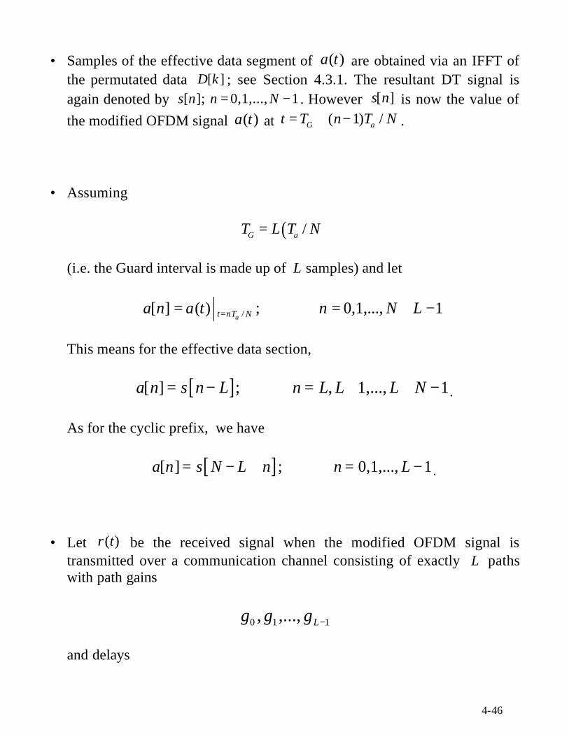
• Samples of the effective data segment of ( )a t are obtained via an IFFT ofthe permutated data [ ]D k ; see Section 4.3.1. The resultant DT signal isagain denoted by [ ]; 0,1,..., 1s n n N= − . However [ ]s n is now the value ofthe modified OFDM signal ( )a t at ( 1) /G at T n T N= + − .

• Assuming

( )/G aT L T N=

(i.e. the Guard interval is made up of L samples) and let

/[ ] ( ) ; 0,1,..., 1at nT Na n a t n N L== = + −

This means for the effective data section,

[ ][ ] ; , 1,..., 1a n s n L n L L L N= − = + + − .

As for the cyclic prefix, we have

[ ][ ] ; 0,1,..., 1a n s N L n n L= − + = − .

• Let ( )r t be the received signal when the modified OFDM signal istransmitted over a communication channel consisting of exactly L pathswith path gains

0 1 1, ,..., Lg g g −

and delays

4-47

0, , 2 , , ( 1)t t L t∆ ∆ − ∆… .

Here/at T N∆ =

is the time-separation between adjacent samples in the DT signal [ ]a n . Itcan be shown that the following row sum yields the samples of ( )r t att n t= ∆ (only one symbol is shown)

0 0 0 0 0 0

1 1 1 1 1 1

[ ], [ 1], , [ 1],|| [0], [1], ..., [ 1]|| [ ], , [ 2],|| [ 1], [0], , [ 2],|| [ 1]

g s N L g s N L g s N g s g s g s N

g s N L g s N g s N g s g s N g s N

− − + − −− − − − −

…… …

1 1 1 1 1

[ ],|| [ 1], , [ ],|| [ 1], , L L L L Lg s N L g s N L g s N L g s N L g− − − − −− − + − − +

O O O O O O… … [ 1]

s N −

where the sign “ || ||• ” are the delimiters for the time interval [ GT ,T]. Let thereceived samples in this interval be denoted by [ ]r n , 0,1,...., 1n N= − , anddefine the vector r as

[0][1]

[ 1]

r

r

r N

= −

r M .

It is observed that

( )1

0

[ ] ; 0,1,..., 1L

m Nm

r n g s n m n N−

=

= − = − ∑

where ( )N

• represents a mod-N operation. This summation is a circularconvolution and is vital to the anti-multipath capability of OFDM.

4-48

• In matrix form, the circular convolution can be written as

1 11

0 0

L Lm m

m mm m

g g− −

−

= =

= =

∑ ∑r P s P W D

where0 10 0 00 00 010 00 01

1 00 0 0

=

P

LLL

M MM M M LL

is a cyclic permutation matrix,

1 2 1

2 4 2( 1)

( 1) ( 1)2 ( 1)( 1)

1 1 1 11

1

1

NN N N

NN N N

N N N NN N N

W W W

W W W

W W W

−

−

− − − −

=

W

LLL

M M M L ML

is the matrix representing DFT with

1 †1N

− =W W ,

and

[0][1]

,

[ 1]

D

D

D N

= −

D M

is the permutated data vector.

4-49

• To detect the data vector D , the receiver performs a DFT of the [ ]r n s.This is equivalent to computing

11

0

11

0

1

0

Lm

mm

Lm

mm

L

m mm

g

g

g

−−

=

−−

=

−

=

=

= = =

∑

∑

∑

R Wr

W P W D

WP W D

Q D

where (show this)

( )

0

21 †

1

1

Nm

N

mm mNm

N mN

W

W

WN

W

−

−

= = =

Q WP W WP W

O

is a diagonal matrix. Consequently, the recovered data can be rewritten as

1

0

L

m mm

g−

=

= = ∑R Q D HD ,

where

4-50

0

11

0

1

L

m mm

N

H

Hg

H

−

=

−

= =

∑H Q O

is also a diagonal matrix whose k-th element,

1

0

Lkm

k m Nm

H g W−

=

= ∑ ,

represents the frequency response of the channel at the subcarrier frequency

k c

a

kf f

T= +

• Since the matrix H is diagonal, the k-th recovered data is simply

[ ] [ ]kR k H D k= .

The result implies that there is no ISI, even though the channel is a non-ideal channel.

• It should be pointed out that in order to successfully detect the data in [ ]R k ,the frequency response kH needs to be estimated. This can be done byinserting a preamble (training symbols) to the data. Alternatively, we canuse differential detection.