4

Fiber Bundles

In the discussion of topological manifolds, one often comes across the useful concept₁ ₂of starting with two manifolds M and M , and building from them a new manifold, using

₁the product topology: M × ₂M . A fiber bundle is a natural and useful generalization of thisconcept.

4.1 Product Manifolds: A Visual Picture

₁ ₂One way to interpret a product manifold is to place a copy of M at each point of M .₂ ₁Alternatively, we could be placing a copy of M at each point of M . Looking at the specific

example of R² = R × R, we take a line R as our base, and place another line at each point of₁ ₂the base, forming a plane. For another example, take M = S¹, and M = the line segment

(0,1). The product topology here just gives us a piece of a cylinder, as we find when we placea circle at each point of a line segment, or place a line segment at each point of a circle.

Figure 4.1 The cylinder can be built from a line segment and a circle.

A More General Concept

A fiber bundle is an object closely related to this idea. In any local neighborhood, a₁fiber bundle looks like M × ₂M . Globally, however, a fiber bundle is generally not a product

manifold. The prototype example for our discussion will be the möbius band, as it is thesimplest example of a nontrivial fiber bundle. We can create the möbius band by startingwith the circle S¹ and (similarly to the case with the cylinder) at each point on the circleattaching a copy of the open interval (0,1), but in a nontrivial manner. Instead of justattaching a bunch of parallel intervals to the circle, our intervals perform a 180° twist as wego around. This gives the manifold a much more interesting geometry.

We look at the object we've formed, and note that locally it is indistinguishable fromthe cylinder. That is, the “twist” in the möbius band is not located at any particular point onthe band; it is entirely a global property of the manifold. Motivated by this example, we seekto generalize the language of product spaces, to include objects like the möbius band whichare only locally a product space. This generalization is what we will come to know as a fiberbundle.

Figure 4.2 The mobius band can also be built from a circle and line segment, but using a moregeneral method of construction.

4.2 Fiber Bundles: The Informal Description

When we build up the language to describe a fiber bundle, we want to regard a fiberbundle as “locally a product space” in the same sense that a manifold is “locally euclidean”.For this reason, the language describing fiber bundles will mimic the language of manifoldsquite closely.

The manifold we are creating will be called the total space, E. It will be constructedfrom a base manifold M, and a fiber F. In our examples of the cylinder and the möbiusband, S¹ is the base manifold, and the interval (o,1) is the fiber. However, since globally thecylinder and möbius band differ, we're definitely going to need some additional data todistinguish them.

We shall find that for a general point q in E, we can directly associate this with apoint p in the base manifold, M. However, we cannot generally associate q with a point inthe fiber, F. This is an important fact which makes the fiber bundle a more general objectthan a product space; M and F are fundamentally different objects, and it can be seenreadily in the case of the möbius band:

θSay we want to parameterize the möbius band by a point on the circle, and a realnumber f in the interval (0,1 θ). Concretely, say = 0 and f = ¾. Now, we transport the point

θ θ →around the möbius band by increasing and keeping f fixed at ¾. When 2π, we shouldθreturn to the same point q in E, since it corresponds to the same and f, and hence the

same q. However, because of the inescapable twist in the band, the point we return to isθassociated with = 0, f = ¼. Our parameterization for F somehow “flips” when we move one

turn around the möbius band.

Figure 4.3 Fiber parameterization on the möbius band is not global.

What you should take away from this is that the parameterization for F only works ina local sense; it does not extend globally. You may be tempted to think “Okay, thisparameterization certainly won't do, but perhaps we're just not looking hard enough. Howdo we know that there is no global fiber parameterization for the möbius band?” Let's saythere existed such a parameterization. Then the set of points f = ¾ would give us a closedloop going around the möbius band. Similarly, the points with fiber-value f = ¼ wouldconstitute another closed loop around the band. However, you can check that any two suchloops around the möbius band must cross at some point, and at this point our fiberparameterization would not be well-defined. Fiber parameterization is not global. In thisway, it is a great deal like coordinate parameterization on a manifold. In a neighborhood ofa point, we can parameterize points in E by (p, f), but when we go to another neighborhood,we use a different parameterization, (p, f´).

How to express this mathematically? First, we associate each point in E with a pointin M, which we can globally do. This association can be accomplished by a projection map: EM (4.1)

which projects points q in E to their associated point p in M. This map is generally not one-to-one, of course; we want it to map entire fibers Fp to points p, capturing the fact that we're

attaching a copy of the fiber F to each point p. We can enforce this condition by thefollowing requirement on the preimage:−1 p⋲F (4.2)

for each p in M. We still want to locally parameterize these fibers, but leave the definitionopen to include different parameterizations of F for different neighborhoods. This is thepart which may be familiar from the standpoint of coordinate parameterization.

When one defines coordinates on manifolds, it is generally accomplished by an opencovering {Ui Φ} and a homeomorphism i for each Ui associating it with an open set of Rn. Wewill do something very similar in the case of fiber bundles. We take an open covering of M,{Ui Φ}, and a set of smooth homeomorphisms, { i}, associating an open set of E given by the

preimage π-¹(Ui) with a product space. Formally,

i :U i×F −1U i (4.3)

ΦSince we have a map i between π-¹(Ui) and Ui × F, we can locally express points in Eusing points in Ui × F. We first project the point q in E to a point p in M, using p = π(q),then find an open neighborhood Uj Φ of p, then there is a corresponding map j whichassociates q with a point in Uj × F, i.e. a pair of points (p, f).

Now, it is possible that we could have chosen a different Uk about p, thus a differentΦmap k associating it with a different point (p, f´) in Uk × F. This is fine, but we need to

understand the relationship between f and f´. In other words, to distinguish the bundleproperly, we need to know about all possible choices of fiber parameterization. In the caseof the cylinder, there was only one fiber parameterization, because the space was globally aproduct manifold. In the case of the möbius band, there are two possible parameterizations,and we can make the transformation explicit byf '=1− f (4.4)

Neither parameterization f nor f´ works globally, but we can cover the circle with twooverlapping segments, and choose one parameterization for one segment, and the oppositefor the other segment.

Changes in the parameterization of the fiber are known as transition functions.These are written formally ast ij=i ° j

−1 :U i∩U j×F U i∩U j×F (4.5)so they smoothly carry a point from one product space to another, in the overlapping regionUi ∩ Uj. However, there are more enlightening ways to look at the transition functions.First of all, note that they carry the point p to itself: p , f ⇢ p , f ' (4.6)

So, it may be more enlightening to think of this as a set of maps from F to itself for eachpoint p in the overlap. Symbolically,t ij p: FF (4.7)

Now, notice that {tij} satisfy group axioms:t ij p[ t jk p]= tik p closure t ii p[ f ]= f identity element (4.8)t ji p=t ij

−1 p inversesWe can now think of {tij(p)} as a group. Specifically, since we are interested in smoothtransition functions, {tij(p)} is a lie group. This group is denoted G, and is called the structuregroup of the fiber bundle. Of course, we can't forget that it is also a map from the fiber toitself. This is a realization of the structure group. This group action is also required to besmooth, since that was an original requirement on the transition functions. To summarizeour repackaging, tij is a mapt ij :U i∩U jG (4.9)

into the structure group G which acts smoothly on the fiber F. The transition functionscharacterize the fiber bundle. In the case of the cylinder, the structure group is just thetrivial group of one element. In the möbius band, the structure group is the group of two

₂elements, Z , given by {1, x}, where x² = 1. In other words, we only have twoparameterizations, and thus only one transition function other than the identity, which is itsown inverse:f ' '=1−1− f = f (4.10)

In these two cases, the structure group is a discrete, finite set of elements, andtherefore the dimensionality of the lie group is zero. Keep in mind that these are verysimple cases of fiber bundles, and generally the lie group consists of a continuous spectrumof transition functions. In other words, we call this a lie group for a reason. Also keep inmind that we have a choice when determining our structure group, since we don't have touse all of the elements. For example, if the fiber bundle is trivial, like the cylinder, we canuse any group G we want, but let it act trivially on the fiber. However, it generally makes themost sense to choose the smallest group that is convenient for our purposes.

4.3 Fiber Bundles: The Bloated Description

We have finally laid out all the pieces we need to describe a fiber bundle. Let's give apreliminary brute-force formal definition, before eventually refining it to look a bit nicer.

A Differential Fiber Bundle (E, π, M, F, G) consists of the following:

1. A differential manifold E called the total space2. A differential manifold M called the base manifold3. A differential manifold F called the fiber4. →A surjective map π: E M called the projection, such that π-¹(p) = Fp ≃ F

5. An open covering {Ui} of M with diffeomorphisms

i :U i×F−1U i (4.11)called local trivializations, with

i p , f = p (4.12)6. A lie group, G, known as the structure group, which acts on the fiber, F.

Finally, there is the requirement that the transition functions,i ° j

−1=t ij p (4.13)are smooth and live in G, the structure group. j f = it ij p⋅ f (4.14)

The base manifold and the fiber tell you exactly what the bundle looks like locally. Atthe level of the base manifold, M, open neighborhoods just look like pieces of Rn, and M'stransition functions tell us precisely how they are sewn together. At the level of the bundle,open neighborhoods are just pieces of Rn × F, and there is an additional sewing operation.We need to glue the fiber Fp over p from the patch Ui to the same fiber Fp from the patchUj. The structure group gives you the additional information required to tell you how to“glue” the fibers together.

Figure 4.4 The transition functions specify precisely how the fibers are sewn together.

4.4 Special Types of Fiber Bundles

In the general case of fiber bundles, F can be any differential manifold, and G can beany lie group that acts on F. By adding further requirements, we can define certain specialbundles.

The Trivial Bundle

Almost unnecessary to include, except that it draws the important connection whichshows that bundles are generalizations of product manifolds. Simply put, a trivial bundle isa product manifold. The base and fiber are interchangeable, and the structure group is thetrivial group. The trivial bundle can be covered with one patch; the entire base manifold.

Φ ΦThe “local trivialization” is really a global trivialization, since covers all of the base. Thetrivial bundle can clearly be formed using any two manifolds as base and fiber.

Vector Bundles

A vector bundle is defined by two restrictions: first, the requirement that F beisomorphic to Rk, i.e. that F is a vector space. Second, that the structure group acts linearlyon the vector space. Because of these two requirements, the transition functions have a k-dimensional representation on the fibers. In other words, the transition functions aresubgroups of GLkR.

Special Case: The Tangent Bundle

Take the base manifold to be M, and the fiber at p to be the tangent space TpM, whichis indeed a vector space. The projection operator sends Tp ⇢M p. For the open covering,we can use the same coordinate patches {Ui} that we use to define the manifold structure ofM.

Figure 4.5 The tangent bundle is an example of a fiber bundle with which we are already familiar.

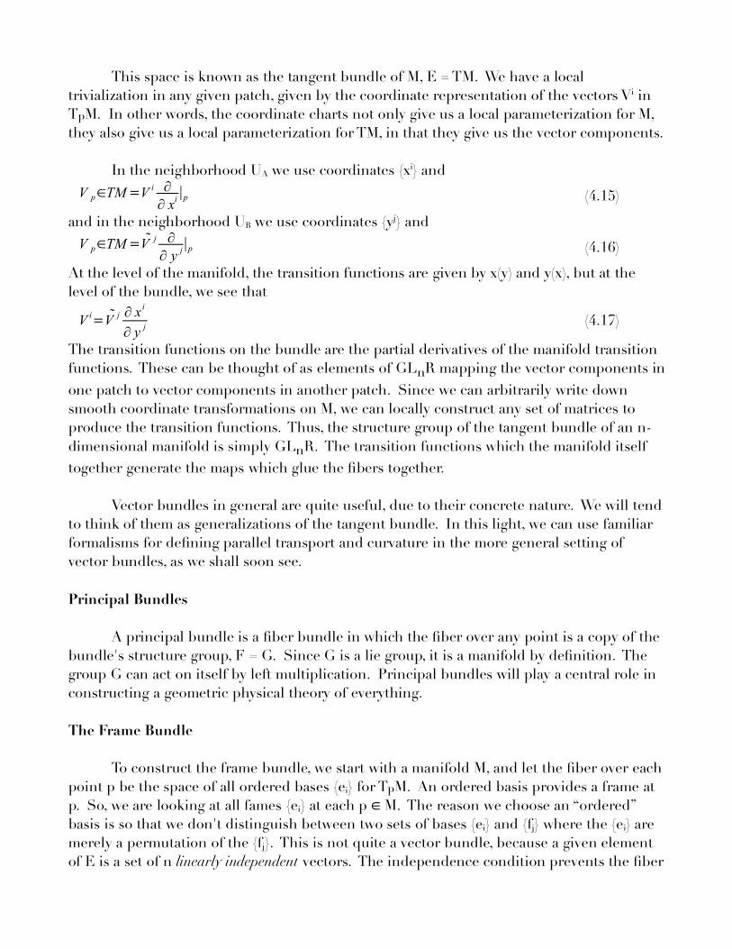
This space is known as the tangent bundle of M, E = TM. We have a localtrivialization in any given patch, given by the coordinate representation of the vectors Vi inTpM. In other words, the coordinate charts not only give us a local parameterization for M,they also give us a local parameterization for TM, in that they give us the vector components.

In the neighborhood UA we use coordinates {xi} and

V p∈TM=V i ∂∂ xi

∣p (4.15)

and in the neighborhood UB we use coordinates {yj} andV p∈TM= V j ∂

∂ y j∣p (4.16)

At the level of the manifold, the transition functions are given by x(y) and y(x), but at thelevel of the bundle, we see that

V i= V j ∂ xi

∂ y j(4.17)

The transition functions on the bundle are the partial derivatives of the manifold transitionfunctions. These can be thought of as elements of GLnR mapping the vector components inone patch to vector components in another patch. Since we can arbitrarily write downsmooth coordinate transformations on M, we can locally construct any set of matrices toproduce the transition functions. Thus, the structure group of the tangent bundle of an n-dimensional manifold is simply GLnR. The transition functions which the manifold itselftogether generate the maps which glue the fibers together.

Vector bundles in general are quite useful, due to their concrete nature. We will tendto think of them as generalizations of the tangent bundle. In this light, we can use familiarformalisms for defining parallel transport and curvature in the more general setting ofvector bundles, as we shall soon see.

Principal Bundles

A principal bundle is a fiber bundle in which the fiber over any point is a copy of thebundle's structure group, F = G. Since G is a lie group, it is a manifold by definition. Thegroup G can act on itself by left multiplication. Principal bundles will play a central role inconstructing a geometric physical theory of everything.

The Frame Bundle

To construct the frame bundle, we start with a manifold M, and let the fiber over eachpoint p be the space of all ordered bases {ei} for TpM. An ordered basis provides a frame atp. So, we are looking at all fames {ei ∈} at each p M. The reason we choose an “ordered”basis is so that we don't distinguish between two sets of bases {ei} and {fj} where the {ei} aremerely a permutation of the {fj}. This is not quite a vector bundle, because a given elementof E is a set of n linearly independent vectors. The independence condition prevents the fiber

from being a vector space. For example, there is no “zero” element in the frame bundle.Note that given any initial basis for TpM, one can find any other by operating on this basisby a suitable element of GLnR:f j=Mij ei (4.18)

Figure 4.6 Any frame can be replaced by the element of the general linear group which gets youthere from the reference frame.

Since the {fj} are a linear combination of the {ej}, and they are linearly independentsince g is nonsingular, the {fj} do indeed form a basis for TpM. Moreover, this exhausts thespace of all frames. If you provide me with any frame {hj}, it is always possible to expresseach hj as a sum of vectors in the original frame. This is equivalent to writing hj = Mij ei,where M is an invertible matrix.

By starting with any fiducial or “point-of-reference” basis, we can get all other basesby acting with elements of GLnR. Then we can label a given frame by the element of GLnRthat got us there from the fiducial frame. In this way, we have shown that the fiber of allframes is nothing but the group GLnR! In other words, the frame bundle is equivalent to aGLnR principal bundle. It will be left as an exercise to make this equivalence more explicit.

The equivalence to which we've just alluded seems useful. Is there any way ofnaturally going the other direction? That is, can we produce some kind of useful fiberbundle from a principal bundle? The answer is yes, from a principal bundle we can buildassociated k-dimensional vector bundles, provided that G has a k-dimensionalrepresentation. This is useful, because vector bundles are much more concretely-describedfiber bundles.

Associated Vector Bundles

The basic idea of constructing associated vector bundles is as follows: Rip out the∈copy of G at each p M. Replace this group fiber by a vector space V of dimension k.

ρChoose the k-dimensional representation k of G. Then choose the transition functions toρbe k(tij) = k × k matrices acting on V.

More formally, let V be a k-dimensional vector space on which G acts via a k-ρdimensional representation, k. Then, given a principal bundle P, define the associated

vector bundle P ×ρ V by starting with P × V and imposing the equivalence relationu ,v ~u⋅g−1 ,g v (4.19)

In a given local neighborhood of u, we can write this equivalence relation in coordinate-form:x ,h ,v ~x , h⋅g−1 ,g v (4.20)

Figure 4.7 A principal bundle has an associated vector bundle for each of its representations.

Problem 4.1 Show that every point in this space, expressed in any coordinate system, isequivalent to a point at the same location on the base, but at the identity point on the G-fiber.Since each point in the space can be expressed in this manner, we have collapsed the G-fiberto a point, while the V-fiber persists. Show that the transition functions for the persisting V-fiber aret ij=k tij (4.21)

The large-scale picture you should have in mind is of a single principal bundle,underneath which sits a multitude of associated vector bundles. For every matrixrepresentation of the structure group G, there exists another associated vector bundle.

4.5 Fiber Bundles: The More Elegant Description

As mathematicians, we are inclined to rigorously define the tools that we use.Specifically, where do they live, and what distinguishes them? For a fiber bundle, we havenot yet explained this. Is it the total space? Is it the collection of spaces? What is thespecific object we are calling the “bundle”, and how does it specify all the underlyingstructure? This is a delicate question, which is why it has been put off until we could get aclearer conceptual picture.

Upon close inspection, you may notice that the fiber bundle is entirely specified bythe projection map, π, subject to a rigorous series of requirements. All the other objects aredefined through π. E and M are its domain and range, and it is required that they are bothdifferential manifolds. Since it is required that E is a differential manifold, it is assumedthat its differential structure is already fixed, but this structure is subject to all therequirements in the definition. F is given by π's preimage of a point in M. Localtrivializations are required to exist and be compatible, but they play a similar role to that ofcoordinate charts on M. Since we required E has a specific topology and differentialstructure, the local trivializations are just all possible maps that are compatible with thisstructure. Once all trivializations are given, this implicitly defines the set of all transitionfunctions, and hence the structure group, G. Thus, all the pieces are truly given by just theprojection map, and for this reason, it is the projection map itself which is often called the“fiber bundle”.

₁ ₂It will sometimes be useful to deem two different bundles π and π to be“equivalent”. We have already done this for the case of the frame bundle and a GLnRprincipal bundle in the previous section (although we did not give much justification). To

₁ ₂do so, we need to be sure that the two total spaces E and E are equivalent differentialmanifolds, i.e. there exists a diffeomorphism: E1E2 (4.22)

However, there must be an equivalence of projection maps as well, so that the base∈ ₁manifolds are defined in the same way. In other words, for all u E ,

1u=2u (4.23)Since the map specifies the bundle, this diffeomorphism equivocates the two bundles. Toget the more general notion of a “bundle map”, we remove the invertibility condition; that is,

Θwe require that be a smooth map between the two bundles, but it need not be bijective.

Problem 4.2 Show that the frame bundle is equivalent to a GLnR principal bundle, as wasstated in section 4.4.

Problem 4.3 Show that the associated vector bundles described in section 4.4 are given by asmooth bundle map from a principal bundle to a vector bundle.

Sections

σA section of a fiber bundle is a map from the base manifold into the total space,picking out a point on the fiber over each point p on the base. Since sections pick outpoints in the total space that lie above the point on the manifold they're mapping from, wecan project back down and recover the original point: p= p (4.24)

For example, a vector field is a section of a tangent bundle.

4.6 Curvature: Generalizing past the Tangent Bundle

Curvature is defined on a manifold by transporting vectors from one tangent space toanother. Thus, curvature is best thought of as a quantity associated with the tangent bundleof a manifold. In this light, we can now generalize this concept to other vector bundles.

In order to make this jump, another conceptual reformulation must occur. When oneΓnormally approaches the concept of a connection over the tangent bundle, i

jk, it is done interms of the transportation properties of coordinate basis vectors. Before we move into moregeneral territory, we need to reformulate our definition of a connection and do so in thecontext of general basis vectors, not necessarily tied to any coordinate system. We define aconnection to tell us how our basis transforms as we move along the manifold. Specifically,if we have a general basis {eμ(p)} for the tangent space TpM, and a basis {e*ν(p)} for thecotangent space Tp ω*M as well, we define the connection by the rate at which the basistransforms as we move in a given direction away from p. This derivative is a vector ofcourse, so we can express it as a linear combination of basis vectors:∇ e=

⊗e (4.25)ΓThe notation here may look somewhat unusual, but it is consistent with the i

jk

ωformulation. The two-indexed object σμ μ σ is a one-form form for each value of and .

=

e∗ (4.26)ωIn other words, can be thought of as an n × n matrix of one-forms. The one-formωcomponent of tells you in which direction you're transporting in the manifold.

ωIt will be useful to determine how the components of transform when we use adifferent set of basis vectors, {fμ(p)}. Each basis vector will be expressible as a linearcombination of the old basis:f =

e (4.27)

Problem 4.4 ω Show that the connection changes in the following manner under such abasis transformation:

=

−1

d −1

(4.28)

Problem 4.5 Show that this expression is consistent with the following transformation law forΓ given by change of coordinates:

jki =∂ xi

∂ yl ∂ y

m

∂ x j∂ y n

∂ xkmnl ∂2 yl

∂ x j∂ xk (4.29)

Remember that you must also perform a coordinate transformation on the index associatedωwith the basis covector that's been contracted with .

The key point to understand is we are no longer changing coordinates on M; we are justchanging the basis we are using for the tangent space. This is the important transition thatwe are required to make before moving to the more general language of vector bundles.

Connections on Vector Bundles

≅Consider a vector bundle V, with vector space fiber F Rk. Let {hμ(p)} be a basis forFp, {eσ(p)} a basis for TpM, and {e*ν(p)} a basis for Tp μ ν*M, where runs from one to k, and

σ ∇and from one to n. Define ν hμ μ to be the rate of change of the th basis vector of theνfiber F in the th direction in the base M. This can be expressed as a linear combination of

the hμ's:∇h=

h (4.30)∇Once again, we can think of the operator as a base-manifold one-form, by contracting its

lower index with the basis covector e*ν(p):∇ h=

h (4.31)where

= e∗ p (4.32)

This may seem repetitive, but only because we've set up the notation so that we'rebasically copying the equations above (4.25 - 4.27) for connections on the tangent bundle.

μ ρ ωNote that the and components of refer to directions in the vector-space fiber, whileνthe component (which we tend to repress) refers to directions in the manifold. If we now

change fiber basisg=

h (4.33)we get the same transformation law (4.28), which we will often express in abstract matrixform:=⋅⋅−1d ⋅−1 (4.34)

ω is a matrix-valued one-form, meaning each of its n² components sits in the cotangentspace of the manifold. The matrix itself also lives in an interesting space, as we will nowexplore.

Let's say we parallel-transport a basis vector along some coordinate direction. Howdo we find out what new vector results? We have seen in the past that we can make amacroscopic translation by performing a large number of infinitesimal translations. This, wehave seen multiple times, results in an exponential map. We cut to the chase, taking theexponential map of the covariant derivative, and acting on a basis vector:h =[exp { x ∇}]h=h x∇ h½ x 2∇2h... (4.35)

ΔWe're omitting the notation for the sum xα ∇ α because it's clear that's what we're doing,and adding more indices will only complicate the expression. We are simply contracting the

Δ ∇vector x with the one-form component of the covariant derivative .

Problem 4.6 Show that the transported vector is found by taking the matrix exponential ofthe connection:h =[exp { x}]

h (4.36)

From problem 4.6 Δ ω we find that (exp{ x }) is a transformation matrix that gives thevalue of a parallel-transported basis vector, given an initial basis vector. We can imaginesetting up a coordinate system in which the basis {gμ} is parallel-transported along thiscurve. In this case, the transition function from the h-basis to the g-basis will just be the

Δ ωmatrix (exp{ x })ρμ.

ωWhat we are attempting to demonstrate here is that exp{ } is a matrix which sits inthe structure group of the vector bundle,

exp {}∈G (4.37)ωwhich means that must live in the lie algebra of the structure group,

∈ℊ (4.38)ωTo summarize, a connection over a vector bundle is specified by a lie-algebra-valued one-

form over the base manifold.

Curvature of Vector Bundles

We are finally ready to define curvature on vector bundles. At this point, we've setthings up to be a fairly straightforward generalization from what we've presumably alreadyseen. First we look back at the more familiar case, where V = TM. After introducing theChristoffel Connection, we parallel-transport a vector along two paths. Comparing Vpath₁ –Vpath₂ gives us the curvature. In component form, the Riemann curvature can be expressedin terms of the Christoffel connection:R jkli =∂k jl

i ∂l jki km

i jlm− lm

i jkm (4.39)

Since R is antisymmetric in its last two indices, we can think of this portion of the tensor asa two-form:R=½ R

dx∧dx=an n×n matrix of two-forms (4.40)

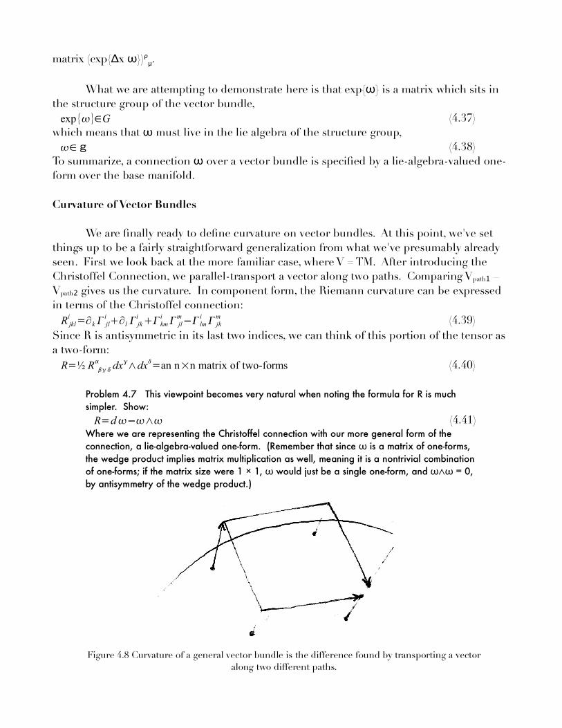
Problem 4.7 This viewpoint becomes very natural when noting the formula for R is muchsimpler. Show:R=d−∧ (4.41)

Where we are representing the Christoffel connection with our more general form of theωconnection, a lie-algebra-valued one-form. (Remember that since is a matrix of one-forms,

the wedge product implies matrix multiplication as well, meaning it is a nontrivial combinationof one-forms; if the matrix size were 1 × ω ω 1, would just be a single one-form, and ∧ω = 0,by antisymmetry of the wedge product.)

Figure 4.8 Curvature of a general vector bundle is the difference found by transporting a vectoralong two different paths.

The connection ∧ω ω ω ω is a matrix of one-forms, and the curvature R = d - is amatrix of two-forms. We generalize this to the language of vector bundles, basically byreplacing the letter R with the symbol Ω. The curvature two-form on a vector bundle V isgiven by:=½ ij

dxi∧dx j=d−∧ (4.42)α βClearly this reduces to the Riemann curvature tensor for V = TM. Note that and

run from one to k, and i and j run from one to n. In other words, these indices refer refer toα βvectors in different spaces; and represent vectors in the fiber, and i and j represent

tangent vectors. Since Ω is a tensor, it is possible to view it as a multilinear map:T p M⊗T p M⊗F pM F p M (4.43)

It rests on basically the same concept as the Riemann curvature; we transport a vectorin the fiber through the manifold on two different paths, specified by two tangent vectors.The difference in the result of the two transports will be found by contracting Ω with thetwo directions and the original vector.

Problem 4.8 When we perform a change of basis in the fiber given by (4.33), show that thecurvature transforms in the following manner:=−1⋅⋅ (4.44)

That is, it transforms as a (1,1) tensor in F*pM ⊗ FpM.

You may be wondering why we care so much how things transform under changes offiber bases. We'd like to be able to construct quantities whose components transform, butwhich can be identified with invariant objects. Currently, the curvature transforms like a(1,1) fiber-valued tensor, and thus we can identify it as such, but the transformation law (4.34)for the connection doesn't lend itself to anything of this nature. To put it more plainly, ω'scomponents are one-forms over the base manifold, but they are not one-forms over the totalspace. When we deal with principal bundles, we will be able to define an invariantconnection which will indeed be associated with a one-form on the total space, but for nowwe have to settle with this half-defined object.

Problem 4.9 Recall that the Λ Λ's all sit in the bundle's structure group, G. If can be foundκby taking the exponential of a lie algebra element, ,

=[exp {}]

(4.45)Show that the transformation law for the connection reduces to=exp {}⋅⋅exp {−}d (4.46)

Note, for small values of κ, this looks like=d [ ,] (4.47)

ω κhighlighting the fact that and are both lie algebra elements, and that the lie algebra isclosed under addition and commutation.

4.7 Parallel Transport on General Fiber Bundles

In the case of a general fiber bundle, we are no longer able to abstract the tangent

bundle's vector language any further, but we can still perform many of the samecalculations, though a bit less concretely. We cannot abstract the quantitative notion ofcurvature to a general fiber bundle, but we can do so the special case of principal bundles.We start by revisiting parallel transport, for the case of a general fiber bundle.

The need for a specification of parallel transport is built into the language of fiber→bundles. The projection map π: E M allows us to definitively say over which point we sit

in the base, but we cannot say definitively at which point we sit in the fiber. F provides alocal coordinate system for points in the neighborhood of p, but these coordinates inthemselves have no substantial meaning, as we can change them at will, thus they can tell usnothing about parallel transport. We need to provide additional information which tells uswhether we are moving up or down the fiber as we move along a path in E. This additionaldata is our final notion of a “connection”.

→Start with a fiber bundle π: E M, with fiber F. Imagine studying the tangent bundleof the total space, TE. This is a fairly complex object; it's the tangent bundle of the totalspace of a fiber bundle. It's worth taking a moment to get your head around this concept.Now, imagine we look at a specific tangent space Tu ∈E at an arbitrary point u E. Furtherimagine that we have a means of decomposing the vector space TuE into a combination oftwo vector spaces:Tu E=V u E⊕Hu E (4.48)

where Vu ≅E TfF is the "vertical" subspace, consisting of directions along the fiber F, and Hu ≅E TpM is the "horizontal" subspace, providing directions along the base M (for some fand p corresponding to the point u in E).

Figure 4.9 The specification of a horizontal subspace defines horizontal transport on a general fiber bundle.

Clearly we haven't been very rigorous, but the idea here is that we are providing aγdefinitive split between “horizontal” and “vertical” transport. Given a curve through E, we

γsay that (t) is parallel-transported if the velocity sits in the horizontal subspace:ddt

∈H t E (4.49)

Thus, if we can provide data which specifies a way of splitting TuE = Vu ⊕E HuE, we havedefined parallel transport in the fiber bundle.

The Connection on a Principal Bundle

→In the special case that π is a principal bundle, P M, with fiber G given by thestructure group, this additional data can, in fact, be expressed as a lie-algebra-valued one-

∈ωform over the total space, g ⊗ ω T*P. Note that we previously defined an which lived inthe cotangent space of the base manifold, T*M, but under the condition that its components

ωtransformed under a change of fiber basis. This new lives in the cotangent space of the∈ωtotal space, T*P.

To find the appropriate lie-algebra-valued one-form, we first choose bundle∈ ∈coordinates (x,g) where x M, g G. In these coordinates, any one-form can be expressed

as:=dx

ij dgij (4.50)

Problem 4.10 We can narrow down the form of our connection by imposing a basicrequirement. When the connection acts on a tangent vector that's just moving vertically alongthe fiber, we want it to return the value of the lie algebra element associated with it. Thisrestricts the set of lie-algebra-valued one-forms we can choose from. A path passing though(x,g) whose tangent vector is the lie algebra element A can be writtenP t =x , g⋅eA t (4.51)

Thus we have the following requirement:

dPdt

=A (4.52)

Show that this implies:ij=gij

−1 (4.53)Thus we can always find parameterization of the fiber such that ω has the following form:=dx

gij−1dgij (4.54)

Alpha contains all of the information about horizontal transport. If we rewrite this expression,we can make contact with our earlier definitions for the connection:=g−1⋅A⋅g dx

gij−1dgij (4.55)

where A is in the lie algebra of G.

We treat Aμ like our old definition of a connection. It transforms annoyingly underfiber reparameterizations (4.34), but the expression (4.55) has just the right form to cancelterms picked up by A's unusual transformation law. We change our notation again,

ωredefining what we mean by the connection :

=g−1⋅A⋅gg ij−1dg ij ,where (4.56)

A=Aa x T a dx (4.57)

Here, {Ta} is a basis for the lie algebra, and {Aμa} is a collection of coefficients for the {Ta}.

ωWe will now show that so defined provides a split of TuP into Vu ⊕P HuP.

First, we write down a basis for HuP:

{ ∂∂ x

Cij ∂∂gij

}∈H u P (4.58)

The {∂/∂xμ} are, of course, directions in the base manifold, while the {∂/∂gij} correspond todirections along the fiber (in a given parameterization). {Cij

μ} are coefficients specified asωinput, selecting a definition of "horizontal". Given a lie-algebra-valued one-form , we can

determine a set of C's, via the following equation:Hu P={V ∈T uP∣V =0}

Problem 4.11 ∈We write a general vector V TuP as

V=ij ∂∂ gij

∂∂ x

C ij ∂∂ gij

(4.59)

When αij ∈ = 0, V HuP, meaning

ij=0⇒V =0 for all {} (4.60)Use (4.56) and (4.57) to compute the coefficients fixing the horizontal subspace:

Cij=−A

a x [T a ]ik g kj (4.61)

The {Aμa ω(x)} is data supplied by , which tells us the Cμ

ij, which nails down thehorizontal subspace HuP.

Hu P={ ∂∂ x

−Aa x [T a ]ik g kj ∂

∂ gij} (4.62)

Parallel Transport on a Principal Bundle

It will now be possible to write down an equation for parallel transport in a principalγbundle. Let (t) be a path in the base M.

t = x1t , x2t ,... , xnt (4.63)γwe want to perform parallel translation in the bundle, lifting (t): →R Γ M to (t): →R P,

Γ γwhere (t) always lies over the point (t) in the base manifold:°= (4.64)

ΓParallel transport requires that the velocity of lives in the horizontal subspace:ddt

∈H t P , for all t (4.65)

More explicitly,ddt= dx

dt∂∂ x

dgij

dt∂

∂ gij= ∂

∂ x−A

a x [T a⋅g ]ij ∂∂ gij

(4.66)

Problem 4.12 Use equation (4.66) to derive the equation of motion for g(t):

dgij

dtdx

dtAa x [T a⋅g ]ij=0 (4.67)

ωGiven a connection specified by A, we simply solve this equation for g(t) todetermine parallel transport on a principal bundle. How now do we determine a rule forassigning curvature to a principal bundle? We cannot simply proceed by analogy, for there isno obvious way of comparing group elements, as there is for vectors. In order to motivateour search for curvature on principal bundles, we take a second look at vector bundles, nowin a more specific context.

4.8 Connections on Associated Vector Bundles

Recall that given a principal bundle, we can build associated vector bundles, whengiven a representation of the structure group. It should come as no surprise that aconnection on a principal bundle induces vector-bundle-connections on all of its associated

ρvector bundles. Given an associated vector bundle with representation , we can performγparallel transport on a vector V at a point p along a curve (t) in the base by the following:

γLook at the point (p = (0), e) in the principal bundle over M, where e is the identityωelement of G. Using the connection , parallel-transport the identity element along the

⊂ ⊂γ Γcurve (t) M, producing the curve (t) P. Act with the representation of the parallel-transported group element on the vector Vp to get the vector Vγ(t), the parallel-transportedvector in the vector bundle. Explicitly,V t= t ⋅V 0 (4.68)

Problem 4.13 Recall that we already have an equation of motion (4.67 Γ) for (t) = g(t), sothese two formulas now yield an equation of motion for V:dVdt

=−dx

dtAa x T a⋅V (4.69)

Remember that a representation of a lie group induces a representation on its lie algebra. Thisρis what is meant by (Ta).

We can rewrite this in terms of covariant differentiation, bydVdt

=dx

dt∂V∂ x

(4.70)

so that (4.69) takes the following form:

∂∂ x

Aa x TaV=0 (4.71)

ωThis is simply the covariant derivative of V. The connection on a principal bundleinduces a connection A = Aa ρ(x) (Ta) on its associated vector bundles. This is the same kindof connection we previously defined for vector bundles. The curvature of an associatedvector bundle can be directly given byF=dA−A∧A (4.72)

ωWhen we constructed , it had a piece corresponding to A, which by itself was not aone-form on the total space, but it was a one-form defined on the base with a connection-like transformation law. As it turns out, this piece is the connection over the associatedvector bundles of the principal bundle, when evaluated in the given representation.

Figure 4.10 A connection on a principal bundle induces connections on all its associated vector bundles.

Curvature on Principal Bundles

Finally, we are in a position to define curvature on principal bundles. Curvature overa principal bundle will be associated with the curvature that it induces over its associatedvector bundles. We state the answer and show that it is consistent:=d −∧ (4.73)

ωwhere now is a lie-algebra-valued one-form over the total space, which can be expressedin a given fiber parameterization like so:=g−1 A gg−1dg (4.74)

Problem 4.14 Show, in this fiber parameterization, the curvature is given by the following:=g−1dA−A∧Ag (4.75)

Remembering that the curvature of a vector bundle transforms like (4.44), the resultof problem 4.14 is motivation enough to define the curvature of a principal bundle in thisway. To summarize this picture, the curvature over a principal bundle is found by the

ωconnection form , a lie-algebra-valued one-form over the total space, P. The curvature Ω isa lie-algebra-valued two-form. For each representation of the structure group G, there exists

an associated vector bundle, with vector bundle connection given by A, which is a lie-∧algebra-valued one-form over the base, and curvature F = dA - A A, a lie-algebra-valued

two-form over the base, and (1,1) tensor over the vector space fiber.