3d wkb solution for fast magnetoacoustic wave behaviour ... · approximation and charpit’s method...

arX

iv:1

607.

0237

9v1

[ast

ro-p

h.S

R]

8 Ju

l 201

6Astronomy & Astrophysicsmanuscript no. McLAUGHLIN˙manuscript˙for˙ArXiv c© ESO 2018September 10, 2018

3D WKB solution for fast magnetoacoustic wave behaviour aro undan X-line

J. A. McLaughlin, G. J. J. Botha, S. Regnier and D. L. Spoors

Department of Mathematics and Information Sciences, Northumbria University, Newcastle upon Tyne, NE1 8ST, UK

Received; Accepted

ABSTRACT

Context. We study the propagation of a fast magnetoacoustic wave in a 3D magnetic field created from two magnetic dipoles. Themagnetic topology contains an X-line.Aims. We aim to contribute to the overall understanding of MHD wavepropagation within inhomogeneous media, specifically aroundX-lines.Methods. We investigate the linearised, 3D MHD equations under the assumptions of ideal and cold plasma. We utilise the WKBapproximation and Charpit’s method during our investigation.Results. It is found that the behaviour of the fast magnetoacoustic wave is entirely dictated by the local, inhomogeneous, equilibriumAlfven speed profile. All parts of the wave experience refraction during propagation, where the magnitude of the refraction effectdepends on the location of an individual wave element withinthe inhomogeneous magnetic field. The X-line, along which the Alfvenspeed is identically zero, acts as a focus for the refractioneffect. There are two main types of wave behaviour: part of the wave iseither trapped by the X-line or escapes the system, and thereexists a critical starting region around the X-line that divides these twotypes of behaviour. For the set-up investigated, it is foundthat 15.5% of the fast wave energy is trapped by the X-line.Conclusions. We conclude that linear,β = 0 fast magnetoacoustic waves can accumulate along X-lines and thus these will be specificlocations of fast wave energy deposition and thus preferential heating. The work here highlights the importance of understanding themagnetic topology of a system. We also demonstrate how the 3DWKB technique described in this paper can be applied to othermagnetic configurations.

Key words. Magnetohydrodynamics (MHD); Magnetic fields; Waves; Sun: corona; Sun: magnetic fields; Sun: oscillations

1. Introduction

It is now clear that magnetohydrodynamic (MHD) wave mo-tions (e.g. Roberts 2004; Nakariakov & Verwichte 2005; DeMoortel 2005) are ubiquitous throughout the solar atmosphere(Tomczyk et al. 2007). Several different types of MHD wavemotions have been observed by various solar instruments: lon-gitudinal propagating disturbances have been seen in SOHOdata (e.g. Berghmans & Clette 1999; Kliem et al. 2002; Wanget al. 2002) and TRACE data (De Moortel et al. 2000) andthese have been interpreted as slow magnetoacoustic waves.Transverse waves have been observed in the corona and chromo-sphere with TRACE (Aschwanden et al. 1999, 2002; Nakariakovet al. 1999; Wang & Solanki 2004), Hinode (Okamoto et al.2007; De Pontieu et al. 2007; Ofman & Wang 2008), SDO data(e.g. McIntosh et al. 2011; Morton et al. 2012, 2015; Morton &McLaughlin 2013, 2014; Thurgood et al. 2014) and these havebeen interpreted as fast magnetoacoustic waves, specifically kinkwaves. These transverse motions have also been interpretedasAlfvenic waves, although this interpretation is subject to discus-sion, e.g. see Erdelyi & Fedun (2007), Van Doorsselaere et al.(2008) and Goossens et al. (2009). Non-thermal line broadeningdue to torsional Alfven waves has been reported by Erdelyiet al.(1998), Harrison et al. (2002), O’Shea et al. (2003) and Jessetal. (2009).It is also clear that the coronal magnetic field plays a funda-mental role in the propagation and properties of MHD waves,

Send offprint requests to: J. A. McLaughlin, e-mail:[email protected]

and to begin to understand this inhomogeneous magnetised en-vironment it is useful to look at the topology (structure) ofthemagnetic field itself. Potential-field extrapolations of the coronalmagnetic field can be made from photospheric magnetograms(e.g. see Regnier 2013) and such extrapolations show the exis-tence of important features of the topology:null points - specificpoints where the magnetic field is zero,separatrices - topologi-cal features that separate regions of different magnetic flux con-nectivity, andX-lines or null lines - extended locations where themagnetic field, and thus the Alfven speed, is zero. Investigationsof the coronal magnetic field using such potential field calcula-tions can be found in, e.g., Brown & Priest (2001), Beveridgeetal. (2002), Regnier et al. (2008) and in a comprehensive reviewby Longcope (2005).

These two areas of scientific study, namely ubiquitous MHDwaves and magnetic topology, will naturally encounter eachother in the solar atmosphere, e.g. MHD waves will propa-gate into the neighbourhood of coronal null points, X-linesandseparatrices. Thus, the study of MHD waves within inhomoge-neous magnetic media is itself a fundamental physical process.Previous works, detailed below, have focused on MHD wave be-haviour in the neighbourhood of null points and separatrices (seereview by McLaughlin et al. 2011). However, less attention hasbeen given to the transient behaviour of MHD waves in the vicin-ity of X-lines in the solar atmosphere. The motivation for thispaper is to address this, i.e. this paper aims to investigatethebehaviour of fast MHD waves around an X-line in order to con-tribute to the overall understanding of MHD wave propagationwithin inhomogeneous media. Note that an X-line is a degen-

1

http://arxiv.org/abs/1607.02379v1

McLaughlin et al.: 3D WKB solution for fast magnetoacousticwave behaviour around an X-Line

erate structure and its existence requires a special symmetry ofthe magnetic field. Thus, given the inherent lack of symmetryinsolar magnetic observations, their existence in the solar atmo-sphere is unlikely. However, X-lines are well studied in otherareas, such as in the Earth’s magnetosphere, e.g. Runov et al.(2003) and Phan et al. (2006).The propagation of fast magnetoacoustic waves in an inhomo-geneous coronal plasma has been investigated by Nakariakov&Roberts (1995), who showed that the waves are refracted intoregions of low Alfven speed (see also Thurgood & McLaughlin2013). In the case of X-lines, the Alfven speed actually drops tozero.MHD waves in the neighbourhood of a single 2D X-point havebeen investigated by various authors. Bulanov & Syrovatskii(1980) provided a detailed discussion of the propagation offastand Alfven waves using cylindrical symmetry. Craig & Watson(1992) mainly considered the radial propagation of them = 0mode (wherem is the azimuthal wavenumber) using a mix-ture of analytical and numerical solutions. They showed thatthe propagation of them = 0 wave towards the null point gen-erates an exponentially large increase in the current density.Craig & McClymont (1991, 1993), Hassam (1992) and Ofmanet al. (1993) investigated the normal mode solutions for bothm = 0 andm , 0 modes with resistivity included. They em-phasise that the current builds as the inverse square of the ra-dial distance from the X-point. All these investigations were car-ried out using cylindrical models in which the generated wavesencircled the X-point and so the cylindrical symmetry meantthat the disturbances can only propagate either towards or awayfrom the X-point. The behaviour of MHD waves around two-dimensional X-points in a Cartesian geometry has been investi-gated by McLaughlin & Hood (2004, 2005, 2006b), McLaughlinet al. (2009) and more recently by Kuzma et al. (2015). Of noteis also McLaughlin & Hood (2006a) who investigated fast MHDwave propagation in the neighbourhood of two dipoles. Theseauthors solved the linearised,β = 0 MHD equations and foundthat the propagation of the linear fast wave is dictated by theAlfven speed profile and that close to the X-point, the wave isattracted to the X-point by a refraction effect. It was also foundthat in this magnetic configuration a proportion of the wave canescape the refraction effect and that the split occurs near the re-gions of very high Alfven speed. However, this study was limitedto 2D. The current paper extends this work to 3D.MHD waves in the vicinity of a 3D null point (e.g. Parnell etal. 1996; Priest & Forbes 2000) have also been investigated.Galsgaard et al. (2003) performed numerical experiments ontheeffect of twisting the spine of a 3D null point, and describedthe resultant wave propagation towards the null. They foundthatwhen the fieldlines around the spine are perturbed in a rota-tionally symmetric manner, a twist wave (essentially an Alfvenwave) propagates towards the null along the fieldlines. Whilstthis Alfven wave spreads out as the null is approached, a fast-mode wave focuses on the null point and wraps around it. Inaddition, Pontin & Galsgaard (2007) and Pontin et al. (2007)performed numerical simulations in which the spine and fan ofa 3D null point are subject to rotational and shear perturbations.They found that rotations of the fan plane lead to current sheetsin the location of the spine and rotations about the spine lead tocurrent sheets in the fan.The WKB approximation is an asymptotic approximation tech-nique which can be used when a system contains a large param-eter (see e.g. Bender & Orszag 1978). Hence, the WKB methodcan be used in a system where a wave propagates through abackground medium which varies on some spatial scale which

is much longer than the wavelength of the wave. There areseveral examples of authors utilising the WKB approximationto compare with numerical results, e.g. Khomenko & Collados(2006) and Afanasyev & Uralov (2011, 2012). Galsgaard et al.(2003) compared their numerical results with a WKB approx-imation and found that, for theβ = 0 fast wave, the wave-front wraps around the null point as it contracts towards it.Theyperform their WKB approximation in cylindrical polar coordi-nates and thus their resultant equations are two-dimensional,since a simple 3D null point is essentially 2D in cylindricalcoordinates. In contrast, this paper will solve the WKB equa-tions for three Cartesian components, and thus we can solve formore general disturbances and more general boundary condi-tions. McLaughlin et al. (2008) utilised the WKB approximationto investigate MHD wave behaviour in the neighbourhood of afully 3D null point. The authors utilised the WKB approxima-tion to determine the transient properties of the fast and Alfvenmodes in a linear,β = 0 plasma regime. From these works, it hasbeen demonstrated that the WKB approximation can provide avital link between analytical and numerical work, and oftenpro-vides the critical insight into understanding the physicalresults.This paper demonstrates the methodology of how to apply theWKB approximation to a general 3D magnetic field configu-ration. We believe that with the vast amount of 3D modellingcurrently being undertaken, applying this WKB technique in3Dwill be very useful and beneficial to the MHD modelling com-munity.This paper describes an investigation into the behaviour offastMHD waves around an X-line using the WKB approximation.The paper has the following outline: In§2, the basic equations,linearisation and assumptions are described, including details ofour equilibrium magnetic field.§3 details the WKB techniqueutilised in this paper as well as its application to the fast wave.The results are given in§4 and the conclusions and discussionare presented in§5. There are multiple appendices (A, B, C)which complement the work in the core text.

2. Governing equations

2.1. Basic equations

The resistive, adiabatic MHD equations for a plasma in the solarcorona are used:

ρ∂v∂t+ ρ (v · ∇) v = −∇p + j × B + ρg ,

∂B∂t= ∇ × (v × B) + η∇2B ,

∂ρ

∂t+ ∇ · (ρv) = 0 ,

∂p∂t+ v · ∇p = −γp∇ · v ,

µ0 j = ∇ × B , (1)

wherev is the plasma velocity,ρ is the mass density,p is theplasma pressure,B is the magnetic induction (usually called themagnetic field),j is the electric current density,g is gravitationalacceleration,γ is the ratio of specific heats,η is the magneticdiffusivity andµ0 is the magnetic permeability in a vacuum.

2.2. Linearised equations and non-dimensionalisation

In this paper, the linearised MHD equations are used to studythe nature of wave propagation. Using subscripts of 0 for equi-

2


Fig. 1. (a) Equilibrium magnetic field in they = 0, xz−plane. Dipoles are located atx = ±0.5. X-point is located atx = 0 andz =√

2a =√

0.5 = 0.707. Red lines indicate the separatrices in this plane. (b) 3D visualisation of the equilibrium magnetic fielddenoting the red separatrices alongy = 0 from (a) and perpendicular to this the blue X-line alongx = 0 from (c). Equilibriummagnetic field is rotationally symmetric about they = 0 axis and thus black curves denote the separatrices in thexy−plane atz = 0.(c) Equilibrium magnetic field shown in thex = 0, yz−plane. Magnetic field is only in thex−direction, hence no arrows. Blue linedenotes the X-line of the formy2+z2 = 2a2. (d) Plot ofBx(0, r) wherer2 = y2+z2. Bx(0, r) changes sign atr =

√2a =

√0.5 = 0.707,

i.e. at location of the X-line. Maximum ofdBx(0, r)/dr occurs atr = 1, whereBx(0, r = 1) = (4/5)5/2 = 0.5724.

librium quantities and 1 for perturbed quantities, equations (1)become:

ρ0∂v1

∂t= −∇p1 + j0 × B1 + j1 × B0 + ρ1g , (2)

∂B1

∂t= ∇ × (v1 × B0) + η∇2B1 , (3)

∂ρ1

∂t+ ∇ · (ρ0v1) = 0 , (4)

∂p1

∂t+ v1 · ∇p0 = −γp0∇ · v1 , (5)

µ0 j1 = ∇ × B1 , (6)

where we note thatv0 = 0. We now consider several simplifi-cations to our system. We will be considering a potential equi-librium magnetic field and so∇ × B0 = j0 = 0. In addition, weignore the effect of gravity on the system, i.e. we setg = 0. Wealso consider an ideal system and so the magnetic diffusivity, η,is set to zero.Furthermore, we consider a cold plasma, i.e.β = 0 plasma ap-proximation, since in the solar coronaβ ≪ 1. Under this as-sumption,p0 = 0 andp1 = p1(x, y, z) from equation (5). We willalso assume the equilibrium gas density,ρ0, is uniform. Note thata spatial variation inρ0 can cause phase mixing (e.g. Heyvaerts& Priest 1983; De Moortel et al. 1999; McLaughlin et al. 2011).There are no assumptions onρ1 = ρ1(x, y, z, t) but we will not

discuss equation (4) further as it can be solved once we knowv1. In fact, under the assumptions ofβ = 0, linearisation andno gravity,ρ1 has no influence on the momentum equation andso the plasma is effectively arbitrarily compressible (Craig &Watson 1992).

We now non-dimensionalise the above equations as follows: letv1 = vv∗1, B0 = BB∗0, B1 = BB∗1, x = Lx∗, y = Ly∗, z = Lz∗,∇ = ∇∗/L and t = t t∗, where we let∗ denote a dimension-less quantity and v,B, L, and t are constants with the dimen-sions of the variable that they are scaling. In addition,ρ0 andp0 are constants as these equilibrium quantities are uniform,i.e.ρ∗0 = p∗0 = 1. We then setB/

√µ0ρ0 = v and v= L/t, which sets

v as a constant equilibrium Alfven speed. Under these scalingst∗ = 1, for example, refers tot = t = L/ v, i.e. the equilib-rium Alfven time taken to travel a distanceL. For the rest of thispaper, we drop the star indices; the fact that they are now non-dimensionalised is understood. Thus, ourβ = 0, ideal, linearised,non-dimensionalised equations are given by:

∂v1

∂t= (∇ × B1) × B0 and

∂B1

∂t= ∇ × (v1 × B0) . (7)

Note that oncev1 is known,ρ1 can be calculated from equation(4).

3


Fig. 2. (a) Shaded surface ofvA(x, y, z0) = |B0(x, y, z0)| in the xy−plane atz0 = 0.1, with local maxima at (x, y, z) = (±a, 0, 0), i.e.the dipoles’ location. (b) Colour contour ofvA(x, 0, z) = |B0(x, 0, z)| in they = 0, xz−plane. Contour is colour coded: 0≤ vA ≤ 0.3(white); 0.3 ≤ vA ≤ 0.5724 (green); 0.5724≤ vA ≤ 2 (yellow); 2 ≤ vA ≤ 30 (orange);vA ≥ 30 (black). Red lines indicate theseparatrices in this plane. (c) Colour contour ofvA(0, y, z) = |B0(0, y, z)| in the x = 0, yz−plane. Blue line indicates the X-line inthis plane. Contour is colour coded in the same way as (b). (d) Plot of |Bx(0, r)| = vA(0, y, z) wherer2 + y2 + z2 and axis displays0.5 ≤ r ≤ 2. Colour coding corresponds to that of (b) and (c), except now black represents|Bx(0, r)| ≤ 0.3.

Equations (7) can be combined to form a single equation:

∂2

∂t2v1 = {∇ × [∇ × (v1 × B0)]} × B0 . (8)

This equation is valid for any 3D potential equilibrium magneticfield, B0. Thus, we now detail our choice ofB0.

2.3. Magnetic equilibrium

We choose a magnetic field created by two magnetic dipoles lo-cated at (x, y, z) = (±a, 0, 0). The mathematical form of our dipo-lar magnetic field comes from the vector potential,A, producedby a magnetic dipole moment,m, whereB0 = ∇ × A and:

A(x) =µ0

4πm × x|x|3

whereµ0 is the permeability of free space andx = (x, y, z). SeeShadowitz (1975) for further details. Thus, the magnetic fieldtakes the formB0 =

(

Bx, By, Bz

)

B/L3, where:

Bx =−2(x + a)2 + y2 + z2

[

(x + a)2 + y2 + z2]5/2+−2(x − a)2 + y2 + z2

[

(x − a)2 + y2 + z2]5/2,

By = −3(x + a) y

[

(x + a)2 + y2 + z2]5/2− 3(x − a) y

[

(x − a)2 + y2 + z2]5/2,

Bz = −3(x + a) z

[

(x + a)2 + y2 + z2]5/2− 3(x − a) z

[

(x − a)2 + y2 + z2]5/2, (9)

whereB is a characteristic field strength,L is the length scalefor magnetic field variations and the loci of the dipoles are lo-cated at±a (2a is the separation of the dipoles). We choosea = 0.5L in our investigation and soa = 0.5 under our non-dimensionalisation. The magnetic field can be seen in Figure1.The equilibrium magnetic field comprises of separatrix surfaces,i.e. the magnetic skeleton, that divide the magnetic regionintofour topologically distinct regions. Figure 1a shows the equilib-rium magnetic field in thexz−plane aty = 0 where the red linesindicate the separatrices in this plane. Note that the equilibriummagnetic field is rotationally symmetric about the axisy = 0,and so the magnetic field geometry in thexy−plane alongz = 0is identical to that of Figure 1a forz → y for y ≥ 0 andz → −yfor y ≤ 0, respectively. This symmetry betweeny andz can alsobe understood from the form of the equations forBy andBz them-selves, which are identical under the mapping(y, z)→ (z, y).

The (red) separatrices cross at an X-point, located at (x, y, z) =(0, 0,

√2a) and at that locationBx(0, 0,

√2a) = By(0, 0,

√2a) =

Bz(0, 0,√

2a) = 0. This X-point, in thexz−plane aty = 0, formsan X-line of the formy2 + z2 = 2a2 in the yz−plane atx = 0.This can be seen in Figure 1b where the blue line denotes theX-line. The X-line is central to the investigation in this paper.Note that the magnetic field is identically zero along the wholeof the X-line. There is no guide-field along the X-line. Note thatthe X-point in they = 0, xz−plane is just a cut across the X-line,and soy2 + z2 ⇒ z2 = 2a2⇒ z =

√2a at x = y = 0.

4


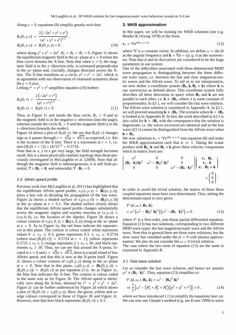
Along x = 0, equations (9) simplify greatly such that:

Bx(0, y, z) =2(

−2a2 + y2 + z2)

(

a2 + y2 + z2)5/2

,

By(0, y, z) = Bz(0, y, z) = 0 , (10)

where alongy2 + z2 = 2a2, Bx = By = Bz = 0. Figure 1c showsthe equilibrium magnetic field in theyz−plane atx = 0 where theblue curve denotes the X-line. Note that whenx = 0, the mag-netic field is in thex−direction only, is orientated perpendicularto theyz−plane and, crucially, changes direction across the X-line. The X-line manifests as a circle,y2 + z2 = 2a2, which isin agreement with our observation of rotational symmetry aboutthey = 0 axis.Letting r2 = y2 + z2 simplifies equation (10) further:

Bx(0, r) =2(

−2a2 + r2)

(

a2 + r2)5/2

,

By(0, r) = Bz(0, r) = 0 . (11)

Thus, in Figure 1c and inside the blue circle,Bx < 0 and sothe magnetic field is in the negativex−direction (into the page),whereas outside the circleBx > 0 and the magnetic field is in thex−direction (towards the reader).Figure 1d shows a plot ofBx(0, r). We see thatBx(0, r) changessign as it passes throughr =

√2a =

√0.5 as expected, i.e. this

is the location of the X-line. There is a maximum atr = 1, i.e.max [Bx(0, r = 1)] = (4/5)5/2 = 0.5724.Note that asx, y or z get very large, the field strength becomessmall; this is a more physically-realistic topology than those pre-viously investigated in McLaughlin et al. (2008). Note thatal-though the magnetic field is inhomogeneous, it is still both po-tential,∇ × B0 = 0, and solenoidal,∇ · B0 = 0.

2.4. Alfven speed profile

Previous work (see McLaughlin et al. 2011) has highlighted thatthe equilibrium Alfven speed profile,vA(x, y, z) = |B0(x, y, z)|,plays a key role in dictating the propagation of the fast wave.Figure 2a shows a shaded surface ofvA(x, y, 0) = |B0(x, y, 0)|in the xy−plane atz = 0.1. The shaded surface clearly showsthat the equilibrium Alfven speed profile changes substantiallyacross the magnetic region and reaches maxima at (x, y, z) =(±a, 0, 0), i.e. the location of the dipoles. Figure 2b shows acolour contour ofvA(x, 0, z) = |B0(x, 0, z)| along in thexz−planeat y = 0. As in Figure 1a, the red lines indicate the separatri-ces in this plane. The contour is colour coded: white representsvalues 0 ≤ vA ≤ 0.3; green represents 0.3 ≤ vA ≤ 0.5724(where max [Bx(0, r)] = 0.5724 atr = 1); yellow represents0.5725≤ vA ≤ 2; orange represents 2≤ vA ≤ 30; and black rep-resentsvA ≥ 30. Thus, we can see that around the X-point, lo-cated atx = 0 andz =

√2a =

√0.5, there is a small island of low

Alfven speed, and that this is zero at the X-point itself. Figure2c shows a colour contour ofvA(0, y, z) along in theyz−planeat x = 0. Note that in this plane,vA(0, y, z) = |B0(0, y, z)| =|Bx(0, y, z)| = |Bx(0, r)| as per equation (11). As in Figure 1c,the blue line indicates the X-line. The contour is colour codedin the same way as for Figure 2b. The Alfven speed is identi-cally zero along the X-line, denoted byr2 = y2 + z2 = 2a2.Figure 2c can be further understood by Figure 2d which showsa plot of |Bx(0, r)| = vA(0, y, z). Here, the green, yellow and or-ange colours correspond to those of Figure 2b and Figure 2c.However, note that here black represents|Bx(0, r)| ≤ 0.3.

3. WKB approximation

In this paper, we will be looking for WKB solutions (see e.g.Bender & Orszag 1978) of the form:

v1 = Veiφ(x, y, z, t) (12)

whereV is a constant vector. In addition, we defineω = ∂φ/∂tas the angular frequency andk = ∇φ = (p, q, r) as the wavevec-tor. Note thatφ and its derivatives are considered to be the largeparameters in our system.One of the difficulties associated with three-dimensional MHDwave propagation is distinguishing between the three differ-ent wave types, i.e. between the fast and slow magnetoacous-tic waves and the Alfven wave. To aid us in our interpretation,we now define a coordinate system (B0, k,B0 × k) wherek isour wavevector as defined above. This coordinate system fullydescribes all three directions in space whenB0 and k are notparallel to each other, i.e.k , λB0, whereλ is some constant ofproportionality. In§3.1, we will consider the fast wave solution.The Alfven wave solution is considered in Appendix A. In§3.1,we will proceed assumingk , λB0. The scenario wherek = λB0is looked at in Appendix B. In fact, the work described in§3.1 isalso valid fork = λB0 with the consequence that the solution isdegenerate, i.e. the waves recovered are identical and so the fastwave (§3.1) cannot be distinguished from the Alfven wave whenk ∝ B0.We now substitutev1 = Veiφ(x, y, z, t) into equation (8) and makethe WKB approximation such thatφ ≫ 1. Taking the scalarproduct withB0, k andB0 × k gives three velocity componentswhich in matrix form are:

ω2 0 0(B0 · k) |k|2 ω2 − |B0|2 |k|2 0

0 0 ω2 − (B0 · k)2

v1 · B0v1 · k

v1 · B0 × k

=

000

.

In order to avoid the trivial solution, the matrix of these threecoupled equations must have zero determinant. Thus, setting thedeterminant equal to zero gives:

F (φ, ω, t,B0, k)

= ω2(

ω2 − |B0|2 |k|2) (

ω2 − (B0 · k)2)

= 0 , (13)

whereF is a first-order, non-linear partial differential equation.Equation (13) has two solutions, corresponding to two differentMHD wave types: the fast magnetoacoustic wave and the Alfvenwave. Note that in general there are three wave solutions, but theslow wave has vanished under theβ = 0 cold plasma approxi-mation. We also do not consider theω = 0 trivial solution.The case where the two roots of equation (13) are the same isexamined in Appendix B.

3.1. Fast wave solution

Let us consider the fast wave solution, and hence we assumeω2, (B0 · k)2. Thus, equation (13) simplifies to:

F (φ, ω, t,B0, k) = ω2 − |B0|2 |k|2

⇒ 12

[

ω2 −(

B2x + B2

y + B2z

) (

p2 + q2 + r2)]

= 0 , (14)

where we have introduced 1/2 to simplify the equations later on.We can now use Charpit’s method (e.g. see Evans 1999) to solve

5


this first-order partial differential equation, where we assume ourvariables depend upon some independent parameters in char-acteristic space. Charpit’s method replaces a first-order partialdifferential equation with a set of characteristics that are a sys-tem of first-order ordinary differential equations. Here, Charpit’sequations take the form:

dφds=

(

ω∂

∂ω+ k · ∂

∂k

)

F , dtds=∂

∂ωF , dx

ds=∂

∂kF ,

dωds= −

(

∂

∂t+ ω∂

∂φ

)

F , dkds= −

(

∂

∂x+ k∂

∂φ

)

F ,

where as previously definedk = (p, q, r) = ∇φ andx = (x, y, z).These ordinary differential equations are subject to the initialconditionsφ = φ0(s = 0), x = x0(s = 0), y = y0(s = 0),z = z0(s = 0), t = t0(s = 0), p = p0(s = 0), q = q0(s = 0),r = r0(s = 0) andω = ω0(s = 0) and are solved numericallyusing a fourth-order Runge-Kutta method.Note that there are no boundary conditions in the traditionalsense: the variables are solved using Charpit’s method (essen-tially a variation on the method of characteristics) and there-sulting characteristics are only dependent upon initial position(x0, y0, z0, t0) and the distance travelled along the characteristic,s. Thus, only initial conditions are required and no boundaryconditions are imposed. The fact that WKB solutions are inde-pendent of boundary conditions is actually an advantage overtraditional numerical simulations where the choice of boundaryconditions can play a significant role. In this paper, we havechosen to illustrate our results in the domain−1 ≤ x ≤ 1,−1 ≤ y ≤ 1, 0≤ z ≤ 2, and this choice is arbitrary.For the fast wave solution and equation (14), Charpit’s equationsare:

dφds= 0 ,

dtds= ω ,

dωds= 0 ,

dxds= −p |B0|2 ,

dyds= −q |B0|2 ,

dzds= −r |B0|2 ,

dpds=

(

Bx∂Bx

∂x+ By∂By

∂x+ Bz

∂Bz

∂x

)

|k|2 ,

dqds=

(

Bx∂Bx

∂y+ By

∂By

∂y+ Bz

∂Bz

∂y

)

|k|2 ,

drds=

(

Bx∂Bx

∂z+ By

∂By

∂z+ Bz

∂Bz

∂z

)

|k|2 , (15)

whereBx, By andBz are the components of our equilibrium field,|B0|2 = B2

x + B2y + B2

z , ω is the angular frequency of our wave,s

is the parameter along the characteristic,p = ∂φ∂x , q = ∂φ

∂y , r = ∂φ∂z

and |k|2 = p2 + q2 + r2. We note thatφ = constant= φ0 andω = constant= ω0, i.e. constant angular frequency. In addition,t = ωs+ t0 where we arbitrarily sett0 = 0, which corresponds tothe leading edge of the wave starting att = 0 whens = 0. Theother six ordinary differential equations are solved numericallyusing a fourth-order Runge-Kutta method.

3.2. Planar fast wave launched from z0 = 0.2

We now solve equations (15) subject to the initial conditions:

φ0 = 0 , ω0 = 2π , −1 ≤ x0 ≤ 1 , −1 ≤ y0 ≤ 1 ,

z0 = 0.2 , p0 = 0 , q0 = 0 , r0 = −ω0/|B0 (x0, y0, z0)| , (16)

where we have chosen arbitrarilyω0 = 2π andφ0 = 0. These ini-tial conditions correspond to a planar fast wave starting atz = z0

Fig. 3. Particle paths for starting points of−1 ≤ x0 ≤ 0 set atintervals of 0.01. The coloured lines represents the particle pathsfor starting points ofx0 = −0.3 (blue) andx0 = −0.298 (red)respectively.

Fig. 5. Particle paths for starting points ofx0 = 0, −1 ≤ y0 ≤0 andz0 = 0.2. The X-line is indicated in blue. The lines for−1 ≤ y0 < −0.6782 have been coloured green to distinguishthem from the lines−0.6782 < y0 ≤ 0 which are black. Theorange and red lines represents the particle paths for a startingpoint ofy0 = −0.85 andx0 = −0.848, respectively.

and propagating in the direction of increasingz. From a mod-elling viewpoint, this choice of initial condition is intended tomimic a disturbance initiated at the ‘photosphere’ ofz = z0.

Note that our choice of a magnetic dipole configuration for theequilibrium magnetic field has two singularities in the fieldat(x, y, z) = (±a, 0, 0) and hencevA → ∞ at these points. Thus,if we were to start our planar wave atz = 0 in thexy−plane, itwould encounter this extreme speed differential. Thus, we gen-erate our waves not atz = 0 but atz = z0, wherez0 is small.This choice still starts the waves in a region of strongly vary-ing Alfven speed, and so this choice results in very little loss ofinsight into the system. In this paper, we choosez0 = 0.2.

6


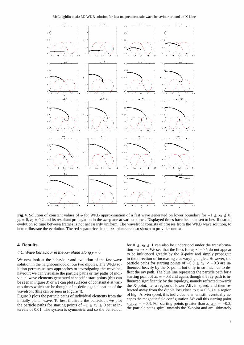
Fig. 4. Solution of constant values ofφ for WKB approximation of a fast wave generated on lower boundary for −1 ≤ x0 ≤ 0,y0 = 0, z0 = 0.2 and its resultant propagation in thexz−plane at various times. Displayed times have been chosen to best illustrateevolution so time between frames is not necessarily uniform. The wavefront consists of crosses from the WKB wave solution, tobetter illustrate the evolution. The red separatrices in the xz−plane are also shown to provide context.

4. Results

4.1. Wave behaviour in the xz−plane along y = 0

We now look at the behaviour and evolution of the fast wavesolution in the neighbourhood of our two dipoles. The WKB so-lution permits us two approaches to investigating the wave be-haviour: we can visualise the particle paths or ray paths of indi-vidual wave elements generated at specific start points (this canbe seen in Figure 3) or we can plot surfaces of constantφ at vari-ous times which can be thought of as defining the location of thewavefront (this can be seen in Figure 4).Figure 3 plots the particle paths of individual elements from theinitially planar wave. To best illustrate the behaviour, weplotthe particle paths for starting points of−1 ≤ x0 ≤ 0 set at in-tervals of 0.01. The system is symmetric and so the behaviour

for 0 ≤ x0 ≤ 1 can also be understood under the transforma-tion −x → x. We see that the lines forx0 ≤ −0.5 do not appearto be influenced greatly by the X-point and simply propagatein the direction of increasingz at varying angles. However, theparticle paths for starting points of−0.5 ≤ x0 < −0.3 are in-fluenced heavily by the X-point, but only in so much as to de-flect the ray path. The blue line represents the particle pathfor astarting point ofx0 = −0.3 and again, though the ray path is in-fluenced significantly by the topology, namely refracted towardsthe X-point, i.e. a region of lower Alfven speed, and then re-fracted away from the dipole loci close tox = 0.5, i.e. a regionof high Alfven speed, this individual element still eventually es-capes the magnetic field configuration. We call this startingpointxcritical = −0.3. For starting points greater thanxcritical = −0.3,the particle paths spiral towards the X-point and are ultimately

7


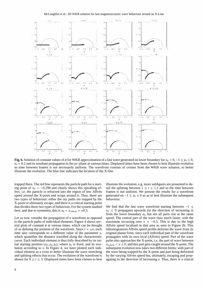
Fig. 6.Solution of constant values ofφ for WKB approximation of a fast wave generated on lower boundary for x0 = 0,−1 ≤ y0 ≤ 0,z0 = 0.2 and its resultant propagation in theyz−plane at various times. Displayed times have been chosen to best illustrate evolutionso time between frames is not necessarily uniform. The wavefront consists of crosses from the WKB wave solution, to betterillustrate the evolution. The blue line indicates the location of the X-line.

trapped there. The red line represents the particle path fora start-ing point of x0 = −0.298 and clearly shows this spiralling ef-fect, i.e. the particle is refracted into the region of low Alfvenspeed around the X-point and wraps around it. Thus, there aretwo types of behaviour: either the ray paths are trapped by theX-point or ultimately escape, and there is a critical starting pointthat divides these two types of behaviour. For the system studiedhere, and due to symmetry, this isx0 = xcritical = ±0.3.

Let us now consider the propagation of a wavefront as opposedto the particle paths of individual elements. Figure 4 showssev-eral plots of constantφ at various times, which can be thoughtof as defining the position of the wavefront. Sincet = ωs, eachtime also corresponds to a different value of the parameters,which quantifies the distance travelled along the characteristiccurve. Each individual element is thus fully described by its ini-tial starting position (x0, y0, z0), wherez0 is fixed, and its evo-lution according tos. In Figure 4, we have plotted each indi-vidual element as a cross to better illustrate the wave stretchingand splitting effects that occur. The evolution of the wavefront isshown for 0≤ t ≤ 3. Displayed times have been chosen to best

illustrate the evolution, e.g. more subfigures are presented to de-tail the splitting between 1≤ t ≤ 1.1 and so the time betweenframes is not uniform. We present the results for a wavefrontgenerated on−1 ≤ x0 ≤ 0 so as to best illustrate the subsequentbehaviour.

We find that the fast wave wavefront starting between−1 ≤x0 ≤ 0 propagates upwards (in the direction of increasingz)from the lower boundaryz0, but not all parts rise at the samespeed. The central part of the wave rises much faster, with themaximum occurring overx = −0.5. This is due to the highAlfven speed localised in that area as seen in Figure 2b. Thisinhomogeneous Alfven speed profile deforms the wave from itsoriginal planar form, since each individual part of the wavefrontpropagates with its own local (Alfven) speed. Part of the wavepulse also approaches the X-point, i.e. the part of wave betweenxcritical < x ≤ 0, and this part gets caught around the X-point. Thesubsequent evolution now takes two different forms: with part ofthe wave being trapped by the X-point and part being deformedby the varying Alfven speed but, ultimately, escaping and prop-agating in the direction of increasingz. Thus, there is a critical

8


(a) (b)

Fig. 7. Particle paths for individual elements generated along (a) −1 ≤ x0 ≤ 1, y0 = 0, z0 = 0.2 and (b) alongx0 = 0,−1 ≤ y0 ≤ 1,z0 = 0.2. The blue line indicates the location of the X-line.

starting point that divides these two types of behaviour,xcritical,in agreement with Figure 3.Let us first consider the part of the wave captured by the X-point,i.e. the part of wave generated betweenxcritical < x ≤ 0 aty = 0andz = z0. This part of the wave propagates upwards and beginsto wrap around the X-point, due to the variation in Alfven speedas seen in Figure 2b. Ultimately, the wave wraps itself around theX-point. As seen in Figure 2d, the Alfven speed is zero at theX-point and so the fast wave cannot cross this point. Consequentlythe X-point acts as a focus for the refraction effect.Let us now consider the part of the wave that escapes an ulti-mate fate of ending up at the X-point, i.e. the wave generatedbetween−1 ≤ x ≤ xcritical at y = 0 andz = z0. This part of thewave continues to propagate upwards and spread out. This partof the wave propagates at a slower speed than at earlier times,again due to the change in the strength of the local Alfven speed.Once above the magnetic skeleton, the wave continues to riseand spread out: the wave is no longer influenced by the X-pointand it has escaped the refraction effect. Ultimately this part ofthe wave leaves the presented domain completely.However, since part of the wave is wrapping around the X-pointand a second part is rising away, the wavefront is being pulledin two different directions. This can be seen in Figure 4 at times1 ≤ t ≤ 1.1. Turning our attention to the behaviour to the right ofthe X-point, we see that the wave continues to spread out: part ofit propagates towards the top right corner and part of it is hookedaround the X-point. We see the wave is stretched between thesetwo destinations. Part of the wave then ultimately wraps aroundthe X-point and the other part propagates away from the dipoleregion. This gives the appearance of the wave splitting, how-ever this is only due to our (discretised) plotting of the wave-front as individual crosses. What has actually occurred is ex-treme stretching of the wavefront. The extreme stretching oc-curs when the wave enters the right-hand region of high Alfv´enspeed, i.e. largevA aroundx = 0.5.When this extreme stretching occurs, the length scales across(perpendicular) to the stretching will rapidly decrease and so thelocal gradients will increase. Hence, if even a small amountofresistivity was included in our system, ohmic heating will actto extract the energy from this location. This would lead to agenuine splitting of the wavefront.Thus, a fast wave generated between−1 ≤ x ≤ 0 alongy = 0and z = z0 propagates into the magnetic region unevenly due

to the inhomogeneity in Alfven speed profile. Part of the waveexperiences a refraction effect, of various magnitudes, due to thenon-uniform local Alfven speed, but ultimately spreads out andpropagates away from the dipolar regions. However, part of thewave is caught by the X-point, refracted into it and accumulateseventually at the X-point. Thus, there is a critical starting pointthat divides these two types of behaviour and investigationof theparticle paths shows that for the system studied here this occursat x0 = xcritical = ±0.3.

We can also use the WKB approximation to plot a solution fora wave generated at−1 ≤ x0 ≤ 1, y0 = 0, z0 = 0.2. This canbe seen in Figure C.1 in Appendix C. As before, each wavefrontconsists of many tiny crosses. Of course, the system is symmet-ric acrossx = 0 and so the explanation of the behaviour is thesame as that above.

4.2. Wave behaviour in the yz−plane along x = 0

We now look at the behaviour of the fast wave solution in thex = 0, yz−plane, i.e. the plane that contains our X-line. This canbe seen in Figure 5 which depicts the particle paths for startingpoints of−1 ≤ y0 ≤ 0 set at intervals of 0.01. Here,x0 = 0andz0 = 0.2. The system is symmetric and so the behaviour for0 ≤ y0 ≤ 1 can also be understood under the transformation−y→ y.

For a wave generated atz0 = 0.2, the straight line segment under

the X-line is bounded byy = ±√

2a2 − z20 = ±

√0.5− 0.22 =

±0.6782. The rays from−1 ≤ y0 < −0.6782 have been colouredgreen to distinguish them from the lines−0.6782 < y0 ≤ 0which are coloured black. We see that for−0.6782< y0 ≤ 0 the(black) generated ray paths propagate upwards from the lowerboundaryz0 and all terminate at the X-line. Here, the individ-ual elements of the wave cannot cross the X-line due to the zeroAlfven speed along those locations and thus this is where thewave accumulates. This propagation can be understood by look-ing at the Alfven speed profile in Figure 2d, which shows thatthemagnitude of the wave speed decreases as an individual elementapproaches the X-line, and is equal to zero atr =

√0.5 = 0.707.

This result, i.e. that fast waves accumulate along X-lines,is anew phenomenon which has not been reported in previous pa-pers.

9


(c) (d)

(a) (b)

Fig. 8. Particle paths for individual elements that start along (a) y0 = −x0. (b) y0 = x0. (c) y0 = x0 looking down on thexy−plane,i.e. there is a line-of-sight effect along thez−direction and X-line is viewed from above. (d) y0 = x0 looking down on thexz−plane,i.e. there is a line-of-sight effect along they−direction and X-line is viewed end-on. Blue line denotes theX-line. Ray paths for|x0| < 0.252 are coloured red and are trapped by the X-line.

For−1 ≤ y0 < −0.6782, the (green) ray paths are deflected bythe varying Alfven speed profile and we observe two types of be-haviour. In Figure 5, the orange and red lines represents thepar-ticle paths from a starting point ofy0 = −0.85 andy0 = −0.848,respectively. Fory0 ≤ −0.85, we see that the ray paths are in-fluenced heavily by the inhomogeneous Alfven speed profile butultimately escape the system. However, fory0 > −0.85 the raypaths refract towards the X-line and terminate there. Thus,as in§4.1, there is a critical starting point that divides these two typesof behaviour. For the system studied here, and due to symmetry,this isy0 = ycritical = ±0.85.Figure 6 shows plots of constantφ at various times. The evolu-tion of the wavefront is shown for 0≤ t ≤ 3. Displayed timeshave been chosen to best illustrate the evolution, e.g. moresub-figures are presented to detail the splitting between 2≤ t ≤ 2.5and so the time between frames is not uniform. We present theresults for a wavefront generated on−1 ≤ y0 ≤ 0 so as to bestillustrate the subsequent behaviour.We find that the fast wave solution starting between−0.6782<y0 ≤ 0.0, i.e. under the X-line, propagates upwards from thelower boundaryz0 and accumulates along the X-line. Note thatelements generated at the X-line itself, i.e.x0 = 0, y0 = 0.6782,z0 = 0.2, have zero local Alfven speed and so remain stationary.For the fast wave solution starting between−1 ≤ y0 < −0.6782,we find that elements of the wavefront generated on−0.85 <y0 < −0.6782 are refracted into the X-line, whereas elementsgenerated−1 ≤ y0 ≤ −0.85 ultimately escape the X-line,although their propagation is modified by the inhomogeneous

Alfven speed profile. From Figure 5, this corresponds toycritical =

−0.85.We can also use the WKB approximation to plot a solution for awave generated atx0 = 0, −1 ≤ y0 ≤ 1 andz0 = 0.2. This canbe seen in Figure C.2 in Appendix C. As before, each wavefrontconsists of many tiny crosses. Of course, the system is symmet-ric acrossy = 0 and so the explanation of the behaviour is thesame as that above.

4.3. Three-dimensional particle paths launched from z0 = 0.2

We can also use our WKB solution to plot the three-dimensional particle paths of individual fluid elements generatedat (x0, y0, z0 = 0.2). In Figure 7a, we see the particle paths for in-dividual elements that begin at starting points of−1 ≤ x0 ≤ 1set at intervals of 0.01 alongy0 = 0 andz0 = 0.2. Thus, thisis a comparison figure for Figure 3 and Figure C.1. Figure 7bdepicts the particle paths for individual elements that begin atstarting points of−1 ≤ y0 ≤ 1 set at intervals of 0.01 alongx0 = 0 andz0 = 0.2, i.e. a comparison figure for Figure 5 andFigure C.2. In both, the blue line indicates the location of the X-line. The results above have shown that it is the X-line that playsa key role, rather than the separatrices. Hence, we do not plot theseparatrices in our 3D figures.Figure 8a and Figure 8b show the particle paths for individualelements that start along the liney0 = −x0 andy0 = x0 respec-tively. We see that, as detailed in§4.1 and§4.2, there are twotypes of ray behaviour: rays can be trapped by the X-line and

10


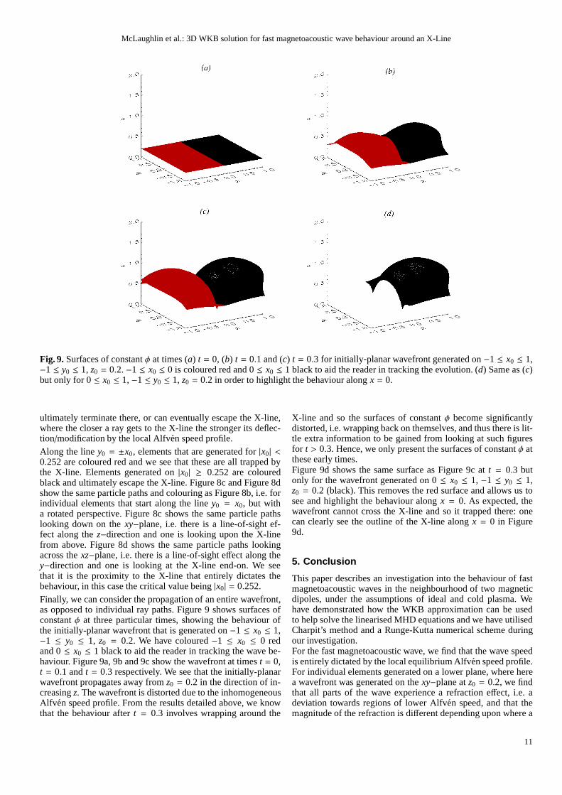
Fig. 9.Surfaces of constantφ at times (a) t = 0, (b) t = 0.1 and (c) t = 0.3 for initially-planar wavefront generated on−1 ≤ x0 ≤ 1,−1 ≤ y0 ≤ 1, z0 = 0.2.−1 ≤ x0 ≤ 0 is coloured red and 0≤ x0 ≤ 1 black to aid the reader in tracking the evolution. (d) Same as (c)but only for 0≤ x0 ≤ 1,−1 ≤ y0 ≤ 1, z0 = 0.2 in order to highlight the behaviour alongx = 0.

ultimately terminate there, or can eventually escape the X-line,where the closer a ray gets to the X-line the stronger its deflec-tion/modification by the local Alfven speed profile.

Along the liney0 = ±x0, elements that are generated for|x0| <0.252 are coloured red and we see that these are all trapped bythe X-line. Elements generated on|x0| ≥ 0.252 are colouredblack and ultimately escape the X-line. Figure 8c and Figure8dshow the same particle paths and colouring as Figure 8b, i.e.forindividual elements that start along the liney0 = x0, but witha rotated perspective. Figure 8c shows the same particle pathslooking down on thexy−plane, i.e. there is a line-of-sight ef-fect along thez−direction and one is looking upon the X-linefrom above. Figure 8d shows the same particle paths lookingacross thexz−plane, i.e. there is a line-of-sight effect along they−direction and one is looking at the X-line end-on. We seethat it is the proximity to the X-line that entirely dictatesthebehaviour, in this case the critical value being|x0| = 0.252.

Finally, we can consider the propagation of an entire wavefront,as opposed to individual ray paths. Figure 9 shows surfaces ofconstantφ at three particular times, showing the behaviour ofthe initially-planar wavefront that is generated on−1 ≤ x0 ≤ 1,−1 ≤ y0 ≤ 1, z0 = 0.2. We have coloured−1 ≤ x0 ≤ 0 redand 0≤ x0 ≤ 1 black to aid the reader in tracking the wave be-haviour. Figure 9a, 9b and 9c show the wavefront at timest = 0,t = 0.1 andt = 0.3 respectively. We see that the initially-planarwavefront propagates away fromz0 = 0.2 in the direction of in-creasingz. The wavefront is distorted due to the inhomogeneousAlfven speed profile. From the results detailed above, we knowthat the behaviour aftert = 0.3 involves wrapping around the

X-line and so the surfaces of constantφ become significantlydistorted, i.e. wrapping back on themselves, and thus thereis lit-tle extra information to be gained from looking at such figuresfor t > 0.3. Hence, we only present the surfaces of constantφ atthese early times.Figure 9d shows the same surface as Figure 9c att = 0.3 butonly for the wavefront generated on 0≤ x0 ≤ 1, −1 ≤ y0 ≤ 1,z0 = 0.2 (black). This removes the red surface and allows us tosee and highlight the behaviour alongx = 0. As expected, thewavefront cannot cross the X-line and so it trapped there: onecan clearly see the outline of the X-line alongx = 0 in Figure9d.

5. Conclusion

This paper describes an investigation into the behaviour offastmagnetoacoustic waves in the neighbourhood of two magneticdipoles, under the assumptions of ideal and cold plasma. Wehave demonstrated how the WKB approximation can be usedto help solve the linearised MHD equations and we have utilisedCharpit’s method and a Runge-Kutta numerical scheme duringour investigation.For the fast magnetoacoustic wave, we find that the wave speedis entirely dictated by the local equilibrium Alfven speedprofile.For individual elements generated on a lower plane, where herea wavefront was generated on thexy−plane atz0 = 0.2, we findthat all parts of the wave experience a refraction effect, i.e. adeviation towards regions of lower Alfven speed, and that themagnitude of the refraction is different depending upon where a

11


fluid element is in the magnetic field configuration. We find thatthere are two main types of wave behaviour:

– Individual fluid elements can be trapped by the X-line, spi-ralling into the X-line due to the refraction effect. These in-dividual elements terminate at the X-line. The wave speeddecreases as an element approaches the X-line and the speedis identically zero at the X-line. Hence, it cannot be crossed.

– Individual fluid elements can escape the system, where ele-ments closer to the X-line have their ray paths modified to agreater extent that those farther away.

Thus,there is a critical starting point that divides these two typesof behaviour. We find that in thexz−plane alongy = 0, this crit-ical starting point isx0 = xcritical = ±0.3, and in the theyz−planealongx = 0, this critical starting point isy0 = ycritical = ±0.85.For starting positions along the linesy0 = ±x0, it was found thatthe critical starting point was|x0| = 0.252.We can also estimate the amount of wave energy trapped by theX-line. For the system studied here, the fraction captured by theX-line will depend upon the critical starting point that divides theparticle paths into those that spiral into the X-line and those thatescape, as well as the overall length of the domain. In this paperwe have set−L ≤ x ≤ L, −L ≤ y ≤ L andz = z0 = 0.2L, whereL is the length of our lower boundary andL = 1 under our non-dimensionalisation. Thus along the linex = 0, ycritical = ±0.85and so 85% of the wave energy is trapped by the X-line, whereasalongy = 0, xcritical = ±0.3 and so 30% is trapped. Thus, morewave energy is trapped from the wave along the X-line thanacross it. Similarly, it was found that the critical starting pointalong the linesy0 = ±x0 was |x0| = 0.252, which correspondsto 17.8% of the wave energy being trapped along a diagonal lineof length

√2L, or 25.2% being trapped along a radial line of

L = 1. Further investigation shows that there is a criticalareasurrounding the X-line, within which all wave elements and thuswave energy is trapped. This critical area corresponds to 0.618L2

across−L ≤ x ≤ L, −L ≤ y ≤ L andz = z0 = 0.2L, which cor-responds to 15.5% of the wave energy generated across an area4 L2 being trapped by the X-line. This critical area is fixed forthe magnetic topology and so the percentage trapped decreasesas one increases the area of the initial wave considered.We have also limited our investigation to understanding thefastwave, but we could have also investigated the second root ofequation (13), i.e. the equations governing the Alfven wave be-haviour. To do so, we would assumeω2

, |B0|2|k|2 and investi-gate the resultant equations. We have included such a derivationin Appendix A although a full investigation is outside the scopeof this current paper.The 3D WKB technique described in this paper can also be ap-plied to other magnetic configurations and we hope that this pa-per has illustrated the potential of exploiting the technique. Inaddition, it is possible to extend the work by dropping the coldplasma assumption. This will lead to a third root of equation(13) which will correspond to the behaviour of the slow magne-toacoustic wave. When the cold plasma assumption is droppedthe fast wave speed will no longer be zero along the X-line, andthus the wave may pass through it. McLaughlin & Hood (2006b)investigated the behaviour of magnetoacoustic waves in a finite-β plasma in the neighbourhood of a two-dimensional X-point. Itwas found that the fast wave could now pass through the X-pointdue to the non-zero sound speed and that a fraction of the inci-dent fast wave was converted to a slow wave as the wave crossedtheβ = 1 layer.There are some caveats concerning the method presented here,i.e. if modellers wish to compare their work with a WKB ap-

proximation, it is essential to know the limitations of suchamethod. Firstly, in linear 3D MHD, we would expect a cou-pling between the fast wave and the other wave types due to thegeometry. However, under the WKB approximation presentedhere, the wave sees the field as locally uniform and so there isno coupling between the wave types. To include the coupling,one needs to include the next terms in the approximation, i.e. thework presented here only deals with the first-order terms of theWKB approximation. Secondly, note that the work here is validstrictly for high-frequency waves, since we tookφ and henceω = ∂φ/∂t to be a large parameter in the system. The extensionto low frequency waves is considered in Weinberg (1962).In this paper we have found that the X-line acts as a focus for therefraction effect and that this refraction effect is a key feature offast wave propagation. Since the Alfven speed drops to identi-cally zero at the X-line, mathematically the wave never reachesthere, but physically the length scales (i.e. the distance between,say, the leading edge and trailing edge of a wave pulse and/orwave train) will rapidly decrease, indicating that all gradients,including current density, will increase at this location.In otherwords, the fast wave, and thus all the fast wave energy, accu-mulates along the X-line. If even a small amount of resistivitywas included in our system, ohmic heating will extract the en-ergy from this location. Thus, we deduce that X-lines will bespecific locations of fast wave energy deposition and preferen-tial heating. This highlights the importance of understanding themagnetic topology of a system and it is at these areas wherepreferential heating will occur. This paper specifically concernsitself with preferential heating at the X-line. However, itis im-portant to note that these are not the only topological locationsat which heat deposition is expected.Finally, we note that an X-line is a degenerate structure anditsexistence requires a special symmetry of the field, and any ar-bitrarily small perturbation to this symmetric configuration willlead to a magnetic topology without a true X-line. The resultingnew topology may exhibit a non-zero component ofB all alongthe original X-line, which may manifest as a quasi-separatrixlayer, or as one or multiple null points. Should the symme-try be broken and the topology changed, we expect that (i)should a quasi-separatrix layer manifest, then we would still getthe extreme stretching described in this paper, since the quasi-separatrix layer would be a location of rapidly changing mag-netic field connectivity, and hence all gradients, including cur-rent density, may increase at these locations. (ii) Should nullpoints appear, then we would expect to recover the results ofMcLaughlin et al. (2008), who studied wave propagation around3D null points.

Acknowledgements. D.L. Spoors acknowledges an Undergraduate ResearchBursary from the Royal Astronomical Society. The authors acknowledge IDLsupport provided by STFC. J.A. McLaughlin acknowledges generous supportfrom the Leverhulme Trust and this work was funded by a Leverhulme TrustResearch Project Grant: RPG-2015-075. J.A. McLaughlin wishes to thank AlanHood for insightful discussions and helpful suggestions regarding this paper.

References

Afanasyev, A. N. & Uralov, A. M. 2011, Sol. Phys.,273, 479Afanasyev, A. N. & Uralov, A. M. 2012, Sol. Phys.,280, 561Aschwanden, M. J., Fletcher,L., Schrijver, C. J. & Alexander, D. 1999, ApJ,520,

880Aschwanden, M. J., De Pontieu, B., Schrijver, C. J. & Title, A. M. 2002,

Sol. Phys.,206, 99Bender, C. M. & Orszag, S. A. 1978, Advanced Mathematical Methods for

Scientists and Engineers, McGraw-Hill, SingaporeBerghmans, D. & Clette, F. 1999, Sol. Phys.,186, 207

12


Beveridge, C., Priest, E. R. & Brown, D. S. 2002, Sol. Phys.,209, 333Brown, D. S. & Priest, E. R. 2001, A&A,367, 339Bulanov, S. V. & Syrovatskii, S. I. 1980, Fiz. Plazmy.,6, 1205Craig, I. J. D. & McClymont, A. N. 1991, ApJ,371, L41Craig, I. J. D. & Watson, P. G. 1992, ApJ,393, 385Craig, I. J. D. & McClymont, A. N. 1993, ApJ,405, 207De Moortel, I., Hood, A. W., Ireland, J. & Arber, T. D. 1999, A&A, 346, 641.De Moortel, I., Ireland, J. & Walsh, R. W. 2000, A&A,355, L23De Moortel, I. 2005, Phil. Trans. Roy. Soc. A,363, 2743De Pontieu, B., McIntosh, S. W., Carlsson, M., Hansteen, V. H., Tarbell, T. D.,

Schrijver, C. J., Title, A. M., Shine, R. A., Tsuneta, S., Katsukawa, Y.,Ichimoto, K., Suematsu, Y., Shimizu, T. & Nagata, S. 2007,Science, 318,1574

Erdelyi, R., Doyle, J. G., Perez, M. E. & Wilhelm, K. 1998, A&A, 337, 287Erdelyi, R. & Fedun, V. 2007,Science, 318, 1572Evans, G., Blackledge, J. & Yardley, P. 1999,Analytical Methods for Partial

Differential Equations, SpringerGalsgaard, K., Priest, E. R. & Titov, V. S. 2003,J. Geophys. Res., 108, 1Goossens, M., Terradas, J., Andries, J., Arregui, I. & Ballester, J. 2009, A&A,

503, 213Harrison, R. A., Hood, A. W. & Pike, C. D. 2002, A&A,392, 319Hassam, A. B. 1992, ApJ,399, 159Heyvaerts, J. & Priest, E. R. 1983, A&A,117, 220Jess, D. B., Mathioudakis, M., Erdelyi, R., Crockett, P. J., Keenan, F. P. &

Christian, D. J. 2009,Science, 323, 1582Khomenko, E. V. & Collados, M. 2006, ApJ,653, 739Kliem, B., Dammasch, I. E., Curdt, W. & Wilhelm, K. 2002, ApJ,568, L61Kuzma, B., Murawski, K. & Solov’ev, A. 2015, A&A,577, A138Longcope, D. W. 2005, Living Rev. Solar Phys. 2,

http://www.livingreviews.org/lrsp-2005-7McIntosh, S. W., De Pontieu, B., Carlsson, M., Hansteen, V.,Boerner, P. &

Goossens, M. 2011,Nature, 475, 477McLaughlin, J. A. & Hood, A. W. 2004, A&A,420, 1129McLaughlin, J. A. & Hood, A. W. 2005, A&A,435, 313McLaughlin, J. A. & Hood, A. W. 2006a, A&A,452, 603McLaughlin, J. A. & Hood, A. W. 2006b, A&A,459, 641McLaughlin, J. A.,Ferguson, J. S. L. & Hood, A. W. 2008, Sol. Phys.,251, 563McLaughlin, J. A., De Moortel, I., Hood, A. W. & Brady, C. S. 2009, A&A, 493,

227McLaughlin, J. A., De Moortel, I. & Hood, A. W. 2011, A&A527, A149McLaughlin, J. A., Hood, A. W. & De Moortel, I. 2011, Space Sci. Rev.,158,

205Morton, R. J., Verth, G., Jess, D. B., Kuridze, D., Ruderman,M. S.,

Mathioudakis, M. & Erdelyi, R. 2012,Nature Communications, 3, 1315Morton, R. J., Tomczyk, S. & Pinto, R. 2015,Nature Communications, 6, 7813Morton, R. J. & McLaughlin, J. A. 2013, A&A,553, L10Morton, R. J. & McLaughlin, J. A. 2014, ApJ,789, 105Nakariakov, V. M. & Roberts B. 1995, Sol. Phys.,159, 399Nakariakov, V. M., Ofman, L., Deluca, E. E., Roberts, B. & Davila, J. M. 1999,

Science, 285, 862Nakariakov, V. M. & Verwichte, E. 2005,Living Reviews in Solar Physics 2,

http://www.livingreviews.org/lrsp-2005-3Ofman, L., Morrison, P. J. & Steinolfson, R. S. 1993, ApJ,417, 748Ofman, L. & Wang, T. J. 2008, A&A,482, L9Okamoto, T. J., Tsuneta, S., Berger, T. E., Ichimoto, K., Katsukawa, Y., Lites,

B. W., Nagata, S., Shibata, K., Shimizu, T., Shine, R. A., Suematsu, Y.,Tarbell, T. D. & Title, A. M. 2007,Science, 318, 1577

O’Shea, E., Banerjee, D. & Poedts, S. 2003, A&A,400, 1065Parnell, C. E., Smith, J. M., Neukirch, T. & Priest, E. R. 1996, Phys. Plasmas 3,

759Phan, T. D., Gosling, J. T., Davis, M. S., Skoug, R. M., Øieroset, M., Lin, R. P.,

Lepping, R. P., McComas, D. J., Smith, C. W., Reme, H. & Balogh, A. 2006,Nature, 439, 175

Pontin, D. I. & Galsgaard, K. 2007,J. Geophys. Res., 112, 3103Pontin, D. I., Bhattacharjee, A. & Galsgaard, K. 2007,Phys. Plasmas, 14, 2106Priest, E. R. & Forbes, T. 2000, Magnetic Reconnection, Cambridge University

PressRegnier, S., Parnell, C. E. & Haynes, A. L. 2008, A&A,484, L47Regnier, S. 2013, Sol. Phys.,288, 481Roberts, B. (2004) SOHO 13:Waves, Oscillations and Small-Scale Transient

Events in the Solar Atmosphere: a Joint View from SOHO and TRACE, ESASP-547, 1

Runov, A., Nakamura, R., Baumjohann, W., Treumann, R. A., Zhang, T. L.,Volwerk, M., Voros, Z., Balogh, A., Glaßmeier, K.-H., Klecker, B., Reme,H. & Kistler, L. 2003, Geophys. Res. Lett.,30, 1579

Shadowitz, A. 1975, The Electromagnetic Field, Dover Publications Inc.Thurgood, J. O. & McLaughlin, J. A. 2013, Sol. Phys.,288, 205Thurgood, J. O., Morton, R. J. & McLaughlin, J. A. 2014, ApJ,790, L2

Tomczyk, S., McIntosh, S. W., Keil, S. L., Judge, P. G., Schad, T., Seeley, D. H.& Edmondson, J. 2007,Science, 317, 1192

Van Doorsselaere, T., Nakariakov, V. M. & Verwichte, E. 2008, ApJ,676, L73Wang, T. J., Solanki, S. K., Curdt, W., Innes, D. E. & Dammasch, I. E. 2002,

ApJ,574, L101Wang, T. J. & Solanki, S. K. 2004, A&A,421, L33Weinberg, S. 1962,Phys. Rev. 6, 1899

Appendix A: Equations governing the Alfv en wave

Let us consider the second root to equation (13) which cor-responds to the Alfven wave solution, and hence we assumeω2, |B0|2 |k|2. This simplifies equation (13) to:

F (φ, x, y, z, p, q, r) = ω2 − (B0 · k)2

⇒ 12

[

ω2 −(

Bxp + Byq + Bzr)2]

= 0 , (A.1)

where we have introduced 1/2 to simplify the equations later on.As in §3.1, we can solve this partial differential equation usingCharpit’s method to reduce the system to seven ordinary differ-ential equations, which can then be solved using, e.g., a Runge-Kutta numerical method. For the Alfven wave solution, Charpit’sequations relevant to equation (A.1) are:

dφds= 0 ,

dtds= ω ,

dωds= 0 ,

dxds= −Bx

(

Bx p + Byq + Bzr)

,

dyds= −By

(

Bx p + Byq + Bzr)

,

dzds= −Bz

(

Bx p + Byq + Bzr)

,

dpds=

(

p∂Bx

∂x+ q∂By

∂x+ r∂Bz

∂x

)

(

Bx p + Byq + Bzr)

,

dqds=

(

p∂Bx

∂y+ q∂By

∂y+ r∂Bz

∂y

)

(

Bx p + Byq + Bzr)

,

drds=

(

p∂Bx

∂z+ q∂By

∂z+ r∂Bz

∂z

)

(

Bx p + Byq + Bzr)

, (A.2)

wherep = ∂φ∂x , q = ∂φ

∂y , r = ∂φ∂z , Bx, By andBz are the components

of our equilibrium field,ω is the angular frequency of our waveands is the parameter along the characteristic. We note thatφ =constant= φ0 andω = constant= ω0, i.e. constant angularfrequency. Thus,t = ωs+ t0 and so one can arbitrarily sett0 = 0,which corresponds to the leading edge of the wave starting att = 0 whens = 0.To generate a planar Alfven wave launched fromz0 = 0.2, onewould then solve equations (A.2) subject to the following initialconditions:

φ0 = 0 , ω0 = 2π , −1 ≤ x0 ≤ 1 , −1 ≤ y0 ≤ 1 , z = z0 ,

p0 = 0 , q0 = 0 , r0 = ω0/|Bz (x0, y0, z0)| ,

where we have (arbitrarily) chosenω0 = 2π andφ0 = 0. Thiscorresponds to a planar Alfven wave initially atz = z0 and prop-agating in the direction of increasingz.

Appendix B: k parallel to B0

In this appendix, we address the scenariok = λB0 in which thevectors of our three-dimensional coordinate system (B0, k,B0 ×

13

http://www.livingreviews.org/lrsp-2005-7

http://www.livingreviews.org/lrsp-2005-3


k) are no longer linearly independent. To do this we considerequation (13):

∂2

∂t2v1 = {∇ × [∇ × (v1 × B0)]} × B0

µ0ρ0,

where we have explicitly includedµ0 and ρ0. Now assumingk = λB0 and applying the WKB approximation from equation12 gives:

ω2v1 = {k × [k × (v1 × B0)]} × B0

µ0ρ0

= (k · B0)2 v1

µ0ρ0− (k · B0) (v1 · B0)

kµ0ρ0

− (k · B0) (k · v1)B0

µ0ρ0+ (k · v1) |B0|2

kµ0ρ0

= λ2 |B0|2

µ0ρ0|B0|2 v1 − λ2 |B0|2

µ0ρ0(v1 · B0) B0

− λ2 |B0|2

µ0ρ0(B0 · v1) B0 + λ

2 (B0 · v1)|B0|2

µ0ρ0B0

= λ2v2A |B0|2 v1 − λ2v2

A (v1 · B0) B0

wherev2A = |B0|2/µ0ρ0. We have explicitly includedµ0 andρ0 to

make the construction ofv2A clear.

Thus, forv1 parallel toB0, i.e.v1 = αB0, we have:

ω2αB0 = λ2v2

A |B0|2αB0 − λ2v2Aα |B0|2 B0 ⇒ ω2 = 0 .

So the longitudinal oscillations (sincev1 ‖ B0 ‖ k) do not propa-gate, i.e. this is the dispersion relation for slow waves under theβ = 0 assumption.Forv1 perpendicular toB0, i.e.v1 · B0 = 0, which are transverseoscillations, we have:

ω2v1 = λ2v2

A |B0|2 v1 ⇒ ω2 = v2A |k|2 .

This is the dispersion relation for a transverse and incompress-ible Alfven wave, i.e.k ‖ B0 ⊥ v1, i.e. it is the same as equation(A.1) under the assumptionB0 ‖ k. However, it is also the dis-persion relation for the fast magnetoacoustic wave propagatingin the direction of the magnetic field. Thus, we cannot distin-guish between these two wave types in this specific scenario.It is also worth noting that even though the coordinate systemwe considered in§3 is not linearly independent whenB0 ‖ k,the result from equation (13) still holds. Under the assumptionk = λB0, equation (13) simplifies to:

F (φ, x, y, z, p, q, r) =(

ω − v2A |k|2

)2= 0 .

So we have a double root and the solution is degenerate, i.e. it isimpossible to distinguish the waves under these conditions, i.e.this is the same as equation (A.1).

Appendix C: Fast wave behaviour in the y = 0,xz−plane and x = 0, yz−plane

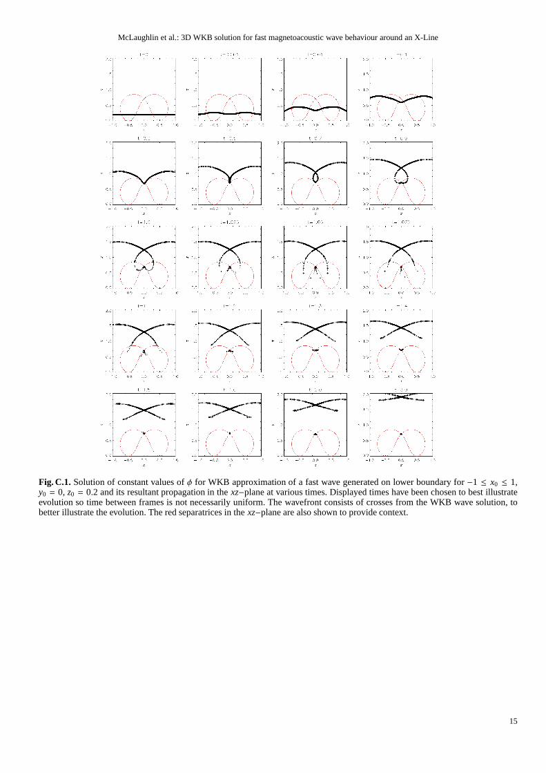
We can use the WKB approximation to plot a solution for a wavegenerated at−1 ≤ x0 ≤ 1, y0 = 0, z0 = 0.2. This can be seenin Figure C.1 which should be compared to Figure 4 in§4.1.We can also use the WKB approximation to plot a solution for awave generated atx0 = 0,−1 ≤ y0 ≤ 1 andz0 = 0.2. This can beseen in Figure C.2 where this should be compared to Figure 6 in§4.2.

14


Fig. C.1. Solution of constant values ofφ for WKB approximation of a fast wave generated on lower boundary for−1 ≤ x0 ≤ 1,y0 = 0, z0 = 0.2 and its resultant propagation in thexz−plane at various times. Displayed times have been chosen to best illustrateevolution so time between frames is not necessarily uniform. The wavefront consists of crosses from the WKB wave solution, tobetter illustrate the evolution. The red separatrices in the xz−plane are also shown to provide context.

15


Fig. C.2. Solution of constant values ofφ for WKB approximation of a fast wave generated on lower boundary for x0 = 0, −1 ≤y0 ≤ 1, z0 = 0.2 and its resultant propagation in theyz−plane at various times. Displayed times have been chosen to best illustrateevolution so time between frames is not necessarily uniform. The wavefront consists of crosses from the WKB wave solution, tobetter illustrate the evolution. The blue line indicates the location of the X-line.

16

3d wkb solution for fast magnetoacoustic wave behaviour ... · approximation and charpit’s method...

Documents