3d vision - princeton university · •advantage: easy to write ... topology •disadvantage:...
TRANSCRIPT

3D Vision

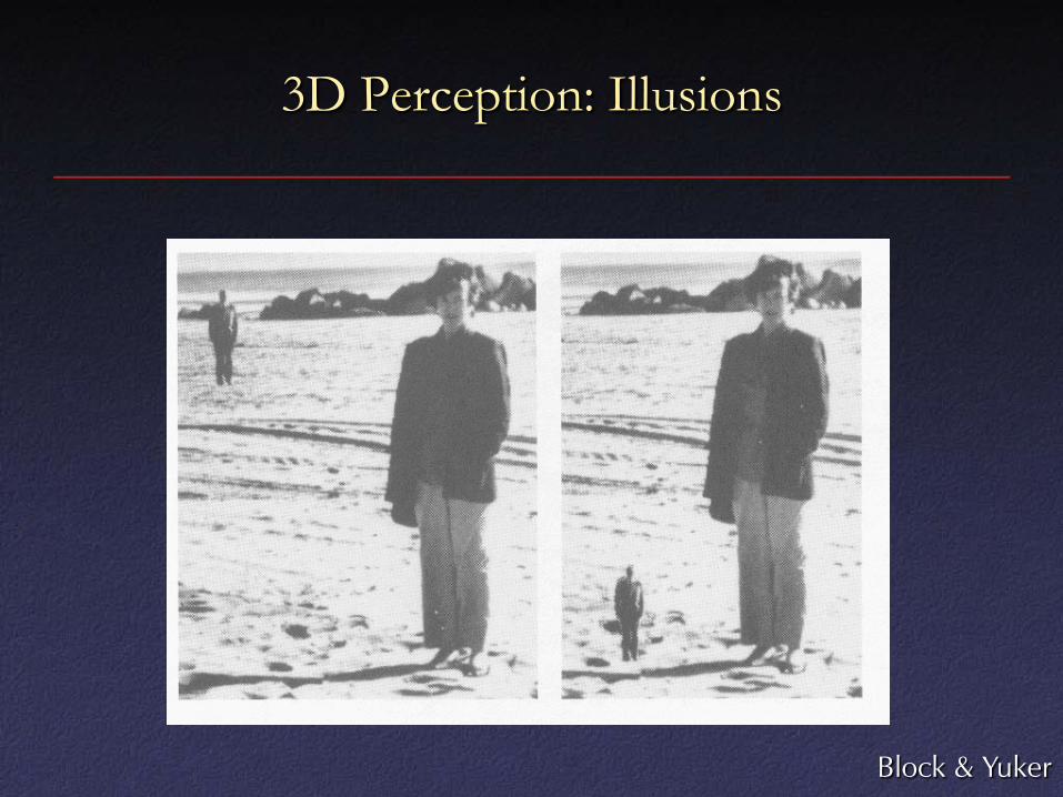
3D Perception: Illusions
Block & Yuker

3D Perception: Illusions
Block & Yuker

3D Perception: Illusions
Block & Yuker

3D Perception: Illusions
Block & Yuker
3D Perception: Illusions
Block & Yuker

3D Perception: Illusions
Block & Yuker

3D Perception: Illusions
Block & Yuker

3D Perception: Illusions
Block & Yuker

3D Perception: Illusions
Block & Yuker

3D Perception: Illusions
Block & Yuker

3D Perception: Conclusions
• Perspective is assumed
• Relative depth ordering
• Occlusion is important
• Local consistency

3D Perception: Stereo
• Experiments show that absolute depth estimation not very accurate – Low “relief” judged to be deeper than it is
• Relative depth estimation very accurate – Can judge which object is closer for stereo disparities
of a few seconds of arc

3D Computer Vision
• Accurate (or not) shape reconstruction
• Some things easier to understand on 3D models than in 2D: – Occlusion
– Variation with lighting (shading)
– Variation with viewpoint
• As a result, some problems become easier: – Segmentation
– Recognition

3D Data Types
• Point Data
• Volumetric Data
• Surface Data

3D Data Types: Point Data
• “Point clouds”
• Advantage: simplest data type
• Disadvantage: no information on adjacency / connectivity

3D Data Types: Volumetric Data
• Regularly-spaced grid in (x,y,z): “voxels”
• For each grid cell, store – Occupancy (binary: occupied / empty)
– Density
– Other properties
• Popular in medical imaging – CAT scans
– MRI
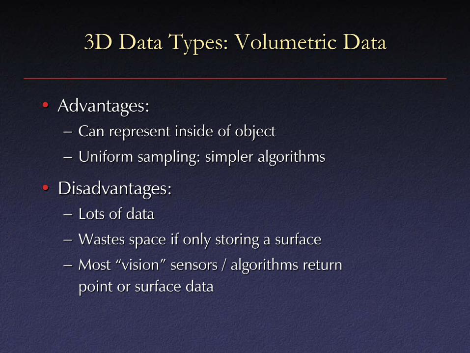
3D Data Types: Volumetric Data
• Advantages: – Can represent inside of object
– Uniform sampling: simpler algorithms
• Disadvantages: – Lots of data
– Wastes space if only storing a surface
– Most “vision” sensors / algorithms return point or surface data

3D Data Types: Surface Data
• Polyhedral – Piecewise planar
– Polygons connected together
– Most popular: “triangle meshes”
• Smooth – Higher-order (quadratic, cubic, etc.) curves
– Bézier patches, splines, NURBS, subdivision surfaces, etc.

3D Data Types: Surface Data
• Advantages: – Usually corresponds to what we see
– Usually returned by vision sensors / algorithms
• Disadvantages: – How to find “surface” for translucent objects?
– Parameterization often non-uniform
– Non-topology-preserving algorithms difficult
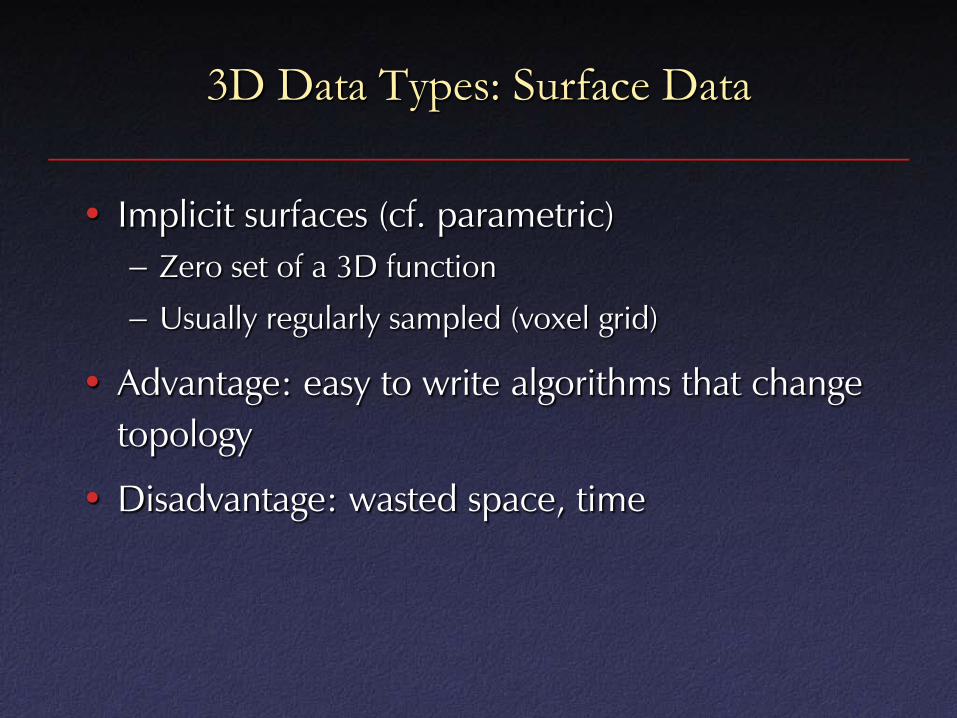
3D Data Types: Surface Data
• Implicit surfaces (cf. parametric) – Zero set of a 3D function
– Usually regularly sampled (voxel grid)
• Advantage: easy to write algorithms that change topology
• Disadvantage: wasted space, time
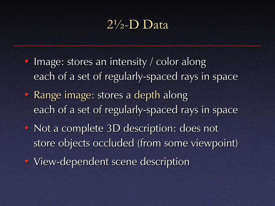
2½-D Data
• Image: stores an intensity / color along each of a set of regularly-spaced rays in space
• Range image: stores a depth along each of a set of regularly-spaced rays in space
• Not a complete 3D description: does not store objects occluded (from some viewpoint)
• View-dependent scene description

2½-D Data
• This is what most sensors / algorithms really return
• Advantages – Uniform parameterization
– Adjacency / connectivity information
• Disadvantages – Does not represent entire object
– View dependent

2½-D Data
• Range images
• Range surfaces
• Depth images
• Depth maps
• Height fields
• 2½-D images
• Surface profiles
• xyz maps
• …

Range Acquisition Taxonomy
Range acquisition
Contact
Transmissive
Reflective Non-optical
Optical
Industrial CT
Mechanical (CMM, jointed arm)
Radar Sonar
Ultrasound MRI
Ultrasonic trackers Magnetic trackers
Inertial (gyroscope, accelerometer)

Range Acquisition Taxonomy
Optical methods
Passive
Active
Shape from X: stereo motion shading texture focus defocus
Active variants of passive methods Stereo w. projected texture Active depth from defocus Photometric stereo
Time of flight
Triangulation

Optical Range Acquisition Methods
• Advantages: – Non-contact
– Safe
– Usually inexpensive
– Usually fast
• Disadvantages: – Sensitive to transparency
– Confused by specularity and interreflection
– Texture (helps some methods, hurts others)

Stereo
• Find feature in one image, search along epipolar line in other image for correspondence

Stereo
• Advantages: – Passive – Cheap hardware (2 cameras) – Easy to accommodate motion – Intuitive analogue to human vision
• Disadvantages: – Only acquire good data at “features” – Sparse, relatively noisy data (correspondence is hard) – Bad around silhouettes – Confused by non-diffuse surfaces
• Variant: multibaseline stereo to reduce ambiguity
Shape from Motion
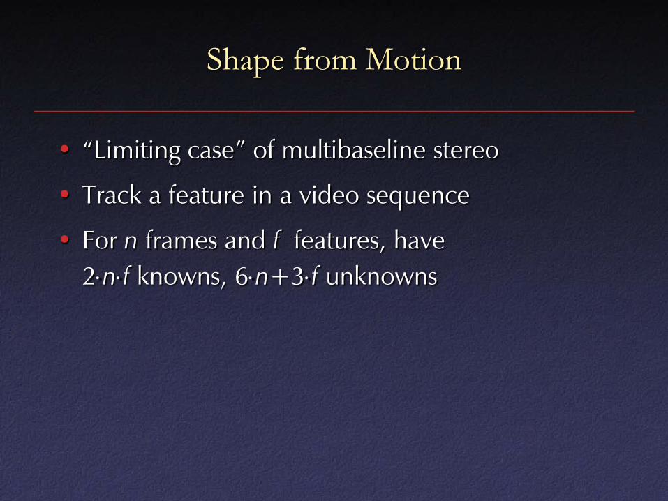
• “Limiting case” of multibaseline stereo
• Track a feature in a video sequence
• For n frames and f features, have 2⋅n⋅f knowns, 6⋅n+3⋅f unknowns

Shape from Motion
• Advantages: – Feature tracking easier than correspondence in far-
away views
– Mathematically more stable (large baseline)
• Disadvantages: – Does not accommodate object motion
– Still problems in areas of low texture, in non-diffuse regions, and around silhouettes

Shape from Shading
• Given: image of surface with known, constant reflectance under known point light
• Estimate normals, integrate to find surface
• Problem: ambiguity

Shape from Shading
• Advantages: – Single image – No correspondences – Analogue in human vision
• Disadvantages: – Mathematically unstable – Can’t have texture
• “Photometric stereo” (active method) more practical than passive version

Shape from Texture
• Mathematically similar to shape from shading, but uses stretch and shrink of a (regular) texture

Shape from Texture
• Analogue to human vision
• Same disadvantages as shape from shading

Shape from Focus and Defocus
• Shape from focus: at which focus setting is a given image region sharpest?
• Shape from defocus: how out-of-focus is each image region?
• Passive versions rarely used
• Active depth from defocus can be made practical

Correspondence and Stereopsis
Original notes by W. Correa. Figures from [Forsyth & Ponce] and [Trucco & Verri]

Introduction
• Disparity: – Informally: difference between two pictures
– Allows us to gain a strong sense of depth
• Stereopsis: – Ability to perceive depth from disparity
• Goal: – Design algorithms that mimic stereopsis

Stereo Vision
• Two parts – Binocular fusion of features observed by the eyes
– Reconstruction of their three-dimensional preimage

Stereo Vision – Easy Case
• A single point being observed – The preimage can be found at the intersection of the
rays from the focal points to the image points
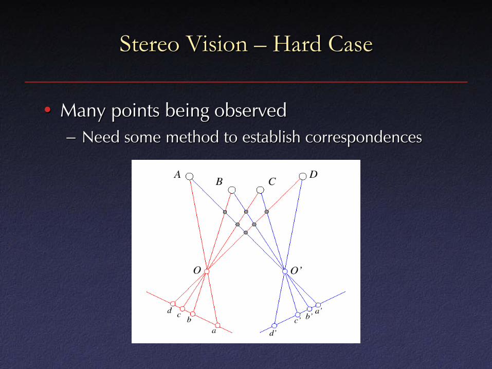
Stereo Vision – Hard Case
• Many points being observed – Need some method to establish correspondences

Components of Stereo Vision Systems
• Camera calibration: next week
• Image rectification: simplifies the search for correspondences
• Correspondence: which item in the left image corresponds to which item in the right image
• Reconstruction: recovers 3-D information from the 2-D correspondences

Multi-Camera Geometry
• Epipolar geometry – relationship between observed positions of points in multiple cameras
• Assume: – 2 cameras
– Known intrinsics and extrinsics
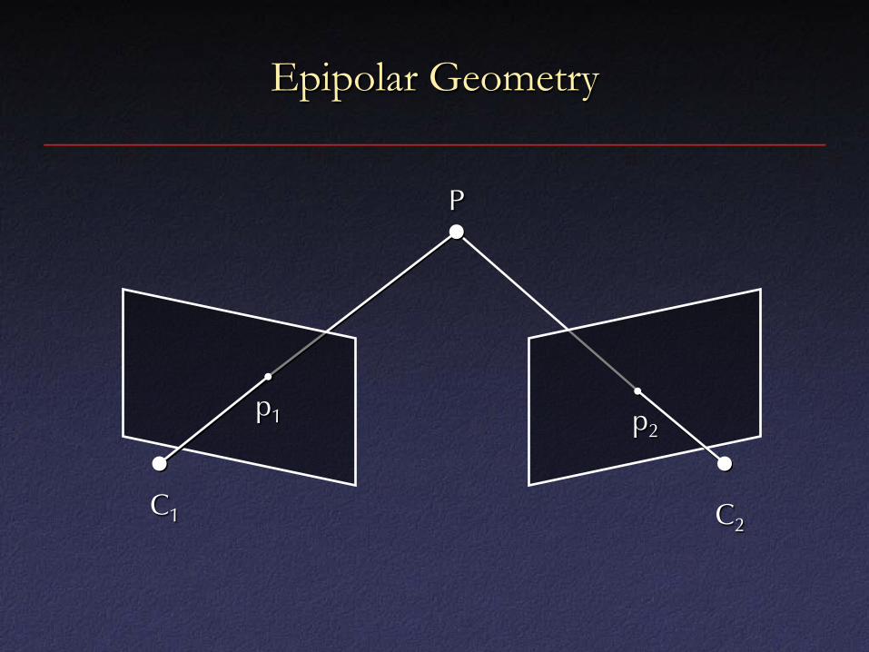
Epipolar Geometry
P
C1 C2
p2 p1
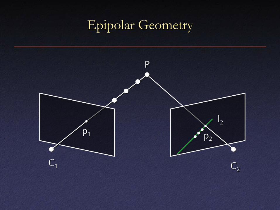
Epipolar Geometry
P
C1 C2
p2 p1
l2
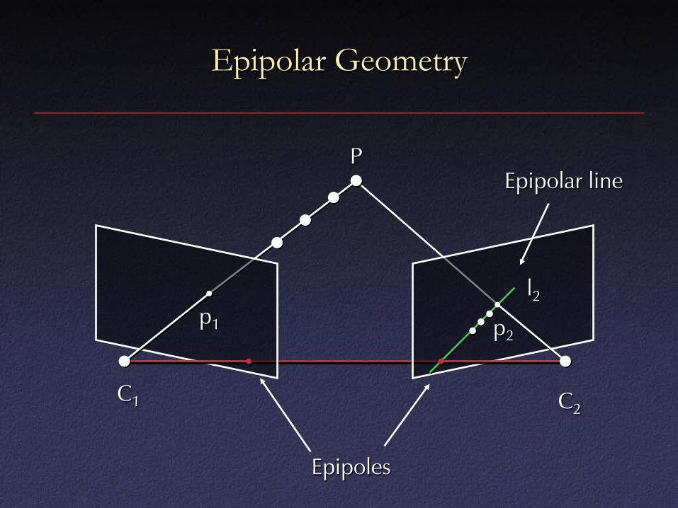
Epipolar Geometry
P
C1 C2
p2 p1
l2
Epipolar line
Epipoles
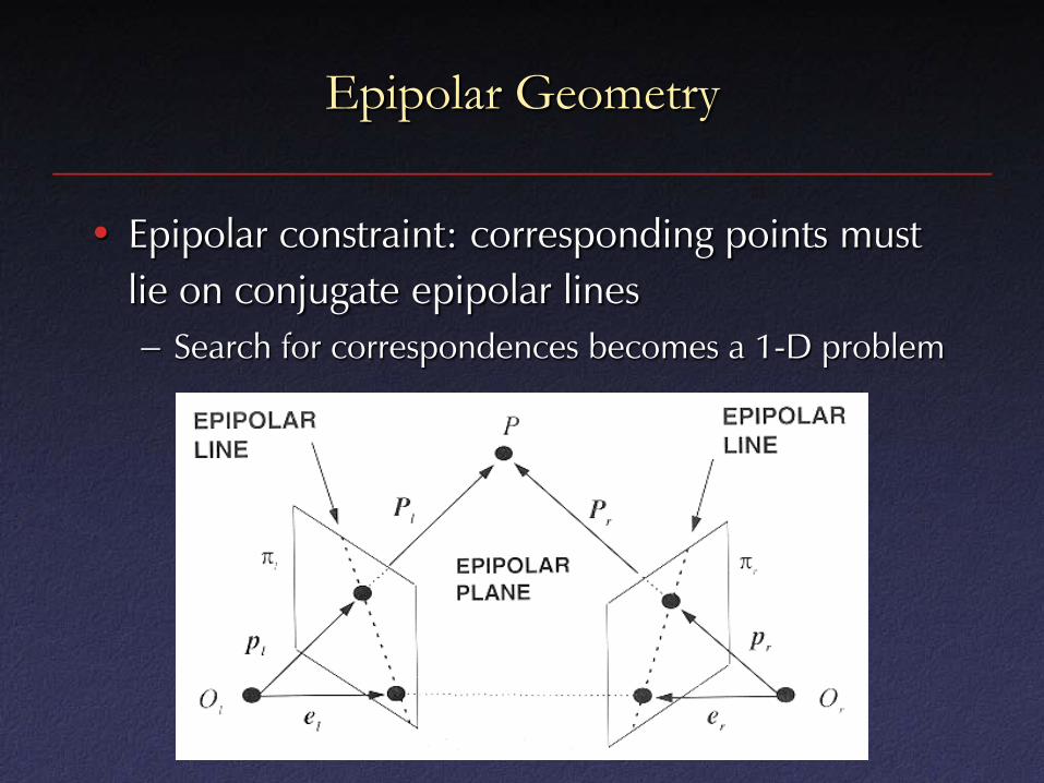
Epipolar Geometry
• Epipolar constraint: corresponding points must lie on conjugate epipolar lines – Search for correspondences becomes a 1-D problem
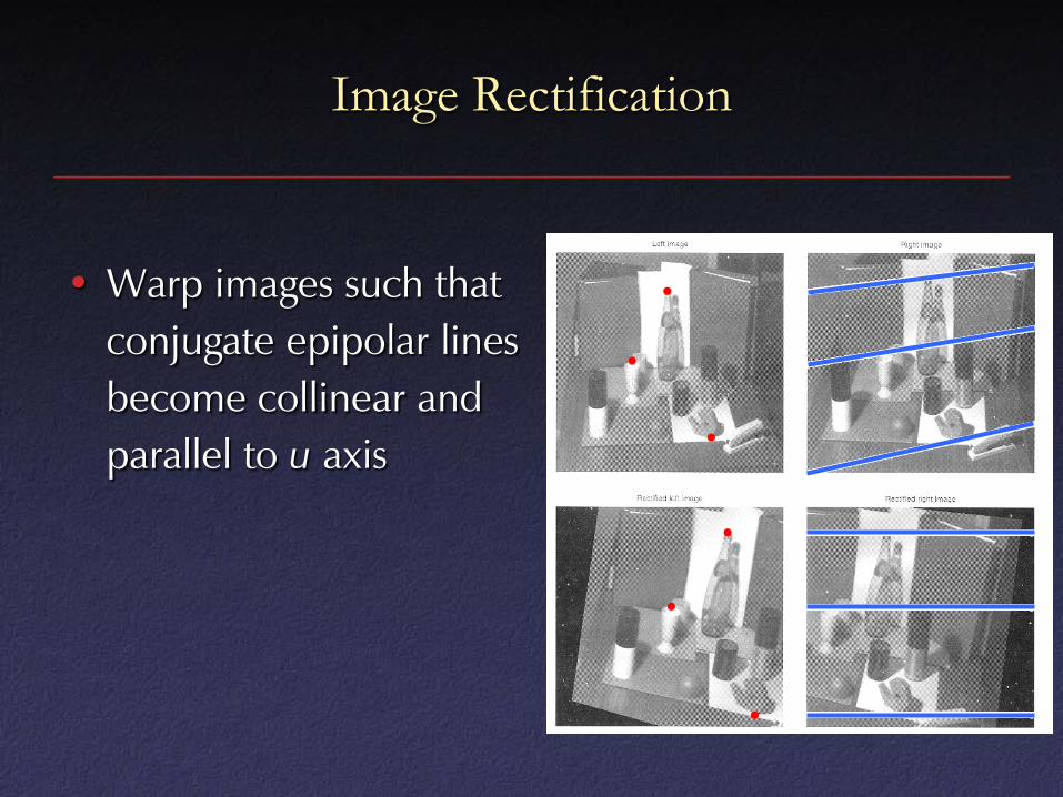
Image Rectification
• Warp images such that conjugate epipolar lines become collinear and parallel to u axis

Disparity
• With rectified images, disparity is just (horizontal) displacement of corresponding features in the two images
– Disparity = 0 for distant points
– Larger disparity for closer points
– Depth of point proportional to 1/disparity

Correspondence
• Given an element in the left image, find the corresponding element in the right image
• Classes of methods – Correlation-based
– Feature-based (next week)

Correlation-Based Correspondence
• Input: rectified stereo pair and a point (u,v) in the first image
• Method: – Consider window centered at (u,v)
– For each potential matching window centered at (u+d,v) in the second image, compute matching score of correspondence
– Set disparity to value of d giving highest score
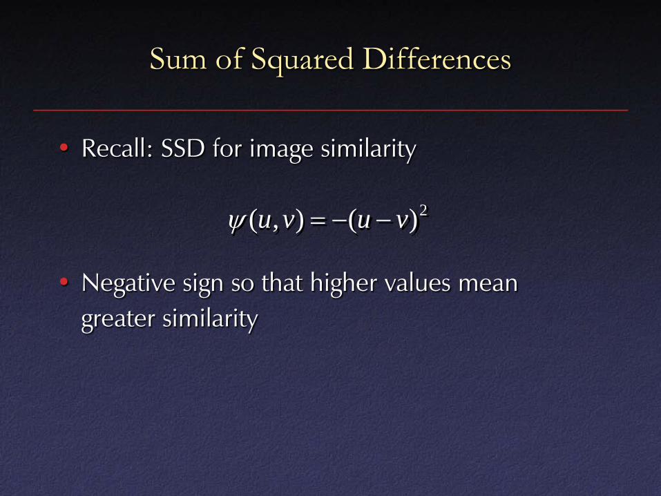
Sum of Squared Differences
• Recall: SSD for image similarity
• Negative sign so that higher values mean greater similarity
2)(),( vuvu −−=ψ

Normalized Cross-Correlation
• Normalize to eliminate brightness sensitivity: where
• Can help for non-diffuse scenes, hurts for perfectly diffuse ones
vu
vvuuvuσσ
ψ ))((),( −−=
)deviation( standard)average(
uuu
u ==
σ

Window-Based Correlation
• For each pixel – For each disparity
• For each pixel in window
– Compute difference
– Find disparity with minimum SSD

Reverse Order of Loops
• For each disparity – For each pixel
• For each pixel in window
– Compute difference
• Find disparity with minimum SSD at each pixel
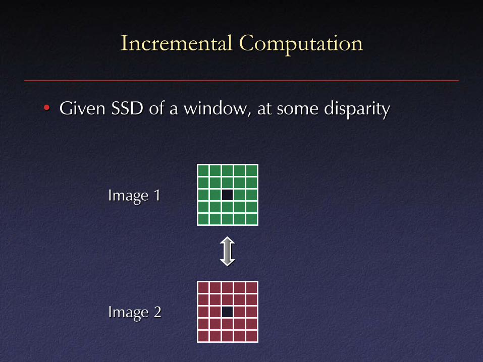
Incremental Computation
• Given SSD of a window, at some disparity
Image 1
Image 2

Incremental Computation
• Want: SSD at next location
Image 1
Image 2

Incremental Computation
• Subtract contributions from leftmost column, add contributions from rightmost column
Image 1
Image 2
+ + + + +
− − − − −
− − − − −
+ + + + +

Selecting Window Size
• Small window: more detail, but more noise
• Large window: more robustness, less detail
• Example:
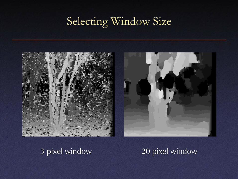
Selecting Window Size
3 pixel window 20 pixel window