3d rotated and standard staggered finite-difference solutions to biot’s

3D rotated and standard staggered finite-difference solutions to Biot’sp

G

oassstrvf

pa

�

©

GEOPHYSICS, VOL. 75, NO. 4 �JULY-AUGUST 2010�; P. T111–T119, 7 FIGS., 2 TABLES.10.1190/1.3432759

oroelastic wave equations: Stability condition and dispersion analysis

areth S. O’Brien1

eamFpfocecwattm

ABSTRACT

Afourth-order in space and second-order in time 3D staggered�SG� and rotated-staggered-grid �RSG� method for the solutionof Biot’s equation are presented. The numerical dispersion andstability conditions are derived using a von Neumann analysis.The exact stability condition is calculated from the roots of a12th-order polynomial and therefore no nontrivial expression ex-ists. To overcome this, a 1D stability condition is usually general-ized to three dimensions. It is shown that in certain cases, the 1Dapproximate stability condition is violated by a 3D SG method.The RSG method obeys the approximate 1D stability conditionfor the material properties and spatiotemporal scales in the exam-ples shown. Both methods have been verified against an analyti-cal solution for an infinite homogeneous porous medium with amisfit error of less than 0.5%.Afree surface has been implement-

a

TtdfghStf

ssgd

ed 10 Fdaptiv

T111

Downloaded 03 Aug 2010 to 193.1.159.167. Redistribution subject to

d to test the accuracy of this boundary condition. It also serves astest of the methods to include high material contrasts. Theethods have been compared with a quasi-analytical solution.or the specific material properties, spatial grid scaling, andropagation distance used in the test, a maximum error of 3.5%or the SG and 4.1% for the RSG was found. These errors dependn the propagation distance, temporal and spatial scales, and ac-uracy of the quasi-analytical solution. No discernable differ-nce was found between the two methods except for time stepsomparable with the stability-criteria threshold time step, the SGas found to be unstable. However, the RSG remained stable forhomogeneous half-space. Time steps, comparable to the stabili-

y criteria, reduce the computational time at the cost of a reduc-ion in accuracy. The methods allow wave propagation to be

odeled in a porous medium with a free surface.

INTRODUCTION

Poroelasticity accounts for the interaction of elastic deformationf a material and viscous fluid flow in the same material. It has widepplications in engineering, physics, and the earth sciences. Morepecifically, in geophysics, poroelastic theory is needed when con-idering earthquake genesis, attenuation properties derived fromeismic waves, reservoir modeling for oil recovery, and CO2 seques-ration. Biot’s theory describes wave propagation in a saturated po-ous medium and accounts for the dissipation of energy due to theiscous pore fluid �Biot, 1962�.Areview of poroelastic theory can beound in Carcione �2007�.

Biot’s equations in terms of the solid displacement u and fluid dis-lacement relative to the solid w for an isotropic poroelastic mediumre given by

u�� fw� ��c�� ·u��2u��M � � ·w �1�

Manuscript received by the Editor 30 June 2009; revised manuscript receiv1University College Dublin, School of Geological Sciences and ComplexA2010 Society of Exploration Geophysicists.All rights reserved.

nd

� fu�mw��M � � ·u�M � � ·w�bw . �2�

he physical constants in equations 1 and 2 describing the poroelas-ic medium are listed in Table 1 along with some of their interdepen-encies. Few exact solutions to equations 1 and 2 exist and are onlyor simplified media and source terms �for example, infinite homo-eneous porous media�. Therefore, to apply Biot’s equations to aeterogeneous medium, numerical techniques must be employed.everal different numerical techniques can be used to solve equa-

ions 1 and 2, but in the present work, we focus solely on a finite-dif-erence solution to Biot’s equations.

Finite-difference methods are a common numerical technique forolving differential equations �Press et al. 2007�. Variables and con-tants in the equations are discretized onto a regular �or irregular�rid, and the spatial and temporal derivatives are replaced by finite-ifference operators acting on variables at specific grid locations.

ebruary 2010; published online 2August 2010.e Systems Lab, Dublin, Ireland. E-mail: [email protected].

SEG license or copyright; see Terms of Use at http://segdl.org/

Nf�ddll�mocticKmtewoMezsacma

mtis

a

Httcopmscm

Tu�

T112 O’Brien

umerous finite-difference techniques have been applied success-ully to the wave equation in different rheologies. Staggered gridsSG�, where different material properties and variables are defined atifferent locations on the grid, are the most common stable finite-ifference scheme for solving the wave equation. This approach al-ows the method to simulate a heterogeneous elastic solid with aarge variation in Poisson’s ratio �Virieux, 1986�. Saenger et al.2000� introduces the rotated staggered grid �RSG� finite-differenceethod for modeling elastic waves. This approach allows the meth-

d to include cracks, pores, and free surfaces without explicitly ac-ounting for them in the numerical method. The main advantage ofhe RSG is higher accuracy for high medium contrasts and highly an-sotropic media. Finite-difference methods have been used to suc-essfully model the viscoelastic wave equation �Emmerich andorn, 1987, Robertsson et al., 1994, and Bohlen, 2002�. The RSGethod also has been applied successfully to viscoelastic and aniso-

ropic wave propagation �Saenger and Bohlen, 2004�.Also, Saengert al. �2007� use an elastic RSG method to simulate the Biot slowave in a microscale rock model where pores were filled with waterr gas hydrates, modeled as an anelastic medium. Dai et al. �1995�,asson et al. �2006�, and Sheen et al. �2006� solve poroelastic wave

quations using a staggered-grid finite-difference approach. Wen-lau and Mueller �2009� implement 2D SG and RSG methods toolve poroelastic wave equations. In this paper, we describe 3D SGnd RSG methods for a poroelastic medium and derive the stabilityondition and dispersion relations. We also compare the numericalethod with an analytical solution and quasi-analytical solution for

n infinite porous medium and a poroelastic half-space.

able 1. Some material parameters needed to describe a poronits and some interdependencies are also listed, and �f, �, b,

are the material-parameter inputs in the RSG finite-differe

Name Units

�s Solid density kg /m3

�f Fluid density kg /m3

� Density kg /m3 ��s�

m Mass coupling coefficient kg /m3 T

� Porosity —

Fluid viscosity Pa s

Permeability m2

T Tortuosity —

b Resistive damping �friction� Pa s /m2

� Lamé constant Pa

�c Lamé constant of saturatedmedium

Pa ��

� Shear modulus Pa

M Fluid storage coefficient Pa Ks�1�� K

� Biot coefficient of effectivestress

— 1�

Ks Solid bulk modulus Pa

Kf Fluid bulk modulus Pa

Kd Drained bulk modulus Pa ��


ROTATED STAGGERED FINITE-DIFFERENCEMETHOD

The set of equations solved in this study using finite-differenceethods are derived from Biot’s equations for poroelastic medium,

he stress-strain relationship for a porous medium, and the pressuren a porous medium �Biot, 1962�. They are expressed in the velocity-tress formulation as

�m� �� f2�vi�m� ij,j�� fbqi�� fp,i, �3�

�m� �� f2�qi�� ij,j��bqi��p,i, �4�

� ij��vi,j�v j,i�� ij��cvk,k

��Mqk,k�, �5�

nd

p��Mvk,k�Mqk,k. �6�

ere, � is the stress, p is pressure, solid velocity v is the time deriva-ive of u, and fluid velocity relative to the solid q is the time deriva-ive of w. A single source term or multiple source terms can be in-luded in one or all of equations 3–6 as a solid stress, fluid pressure,r solid and/or fluid forces. The exact 3D stability condition and dis-ersion relation have not been derived yet for either the SG or RSGethod. Therefore, the stability and the effect of numerical disper-

ion on the solution have yet to be fully quantified. At low frequen-ies �typically the seismic band�, a wave propagating across a porousedium will create laminar flow in the pore space, implying that vis-

cous boundary layers need not be considered. Athigher frequencies, this effect cannot be ignoredbut is not considered in the implementations dis-cussed above. Biot �1956a, 1965b� provides thetheory of elastic wave propagation in porous me-dia for low- and high-frequency ranges. We alsowill not consider the viscous boundary layer be-cause it is not large for the seismic frequencyband.

From equations 3–6, we have four variables �v,q, � , and p� and eight material parameters ��, �f,m, b, �, �, M, and ��, which are distributed on thegrid depending on the finite-difference imple-mentation. Distribution of the parameters neededis shown in Figure 1 for both implementations. Inthe staggered grid, velocity components are lo-cated at different points, with each being half agrid point from the corner in the appropriate com-ponent direction. Normal stresses are located onthe corner and shear stresses are located in thecenter of the appropriate plane. For the rotatedstaggered grid, stress and pressure are located onthe node corners and solid and fluid velocities arelocated on the node midpoints. In both methods,all material parameters are located on the nodecorners. Derivative directions for the RSG alsoare shown in Figure 1 and are described inSaenger et al. �2000�. We use a fourth-order inspace and second-order in time implementationwith �x, �y, and �z being the spatial grid steps

dium. The�, M, and

ethod.

��f

�Ks /Kf��1

s

us mem, �,

nce m

—

—

�1��

�f /�

—

—

—

—

/

—

�2M

—

d /Ks�

Kd /K

—

—

2 /3�


ad

I

esdlptomaatsAC�Tm�i

Wicpbbtq

sftdedpt

a

E

R

Ffr

3D FD methods for Biot’s wave equations T113

nd �t is the temporal time step. Equations 3–6 then can be written iniscretized form for the RSG method as

vt��t/2i�x��x/2,y��y /2,z��z/2��vt��t/2

i�x

��x/2,y��y /2,z��z/2�� t

m� � � f2�

� �mDj� ij�x,y,z�� fbqi�x��x/2,y��y /2,z

��z/2�� fDip�x,y,z��, �7�

qt��t/2i�x��x/2,y��y /2,z��z/2��qt��t/2

i�x

��x/2,y��y /2,z��z/2�� t

m� � � f2�

� �� fDj� ij�x,y,z�� bqi�x��x/2,y��y /2,z

��z/2�� Dip�x,y,z��, �8�

� t��tij�x,y,z�� t

ij�x,y,z��t��Dkvk�x��x/2,y

��y /2,z��z/2��Dkvk�x��x/2,y

��y /2,z��z/2��t� ij��cDkvk�x

��x/2,y��y /2,z��z/2��MDkqk�x

��x/2,y��y /2,z��z/2��, �9�

pt��t�x,y,z��pt�x,y,z��t��MDkvk�x��x/2,y

��y /2,z��z/2��MDkqk�x��x/2,y

��y /2,z��z/2�� . �10�

n equations 7–10, the tilde over variables indicates a time average:

qi�1

2�qi

t��t/2�qit��t/2� . �11�

The corresponding equations for the SG method can be derivedasily from equations 7–10 by placing the variables in their corre-ponding SG locations. Source terms can be added to equations 7–10epending on the specific source implementation that is to be simu-ated. Because the material constants are not defined on all necessaryoints, they are interpolated to these locations in the discrete equa-ions above �indicated by the overbar� using an arithmetical averager a harmonic average. Moczo et al. �2002� show that for a displace-ent-stress finite-difference scheme, harmonic averages are more

ccurate. All results presented in this work use the harmonic aver-ge. Derivative operators for both the SG and RSG methods in equa-ions 7–10 are given in the appendix. The system of equations de-cribed above behaves differently at different time and spatial scales.

system that acts in this manner is called stiff and is discussed byaricone and Quiroga-Goode �1995� and Wenzlau and Müller

2009�. The Biot slow wave at low frequency behaves diffusively.he Biot frequency �Biot, 1962� defined for homogeneous porousedia and given in equation 12 defines the diffusive regime with��B implying that the friction is dominating and the slow P-wave

s diffusive:


�B�b

T� f. �12�

hen the friction is decreased or the source frequency is sufficientlyncreased, the slow P-wave becomes propagative. However, as dis-ussed above, the viscous layers in a real material would become im-ortant, but this effect can be omitted for the seismic frequencyand. For the sake of completeness, several examples are shown inoth regimes. However, it must be remembered that the above equa-ions should include the viscous boundary layers in the high-fre-uency regime.

DISPERSION ANALYSIS AND STABILITYCONDITION

The accuracy and stability of any finite-difference numericalcheme depend heavily on 1� the system of equations, 2� finite-dif-erence operators, 3� order of the finite-difference operators, 4� spa-ial and temporal grid steps, and 5� material contrasts. To quantifyispersion and stability of the finite-difference solutions of Biot’squations, we perform a von Neumann analysis. Substituting theisplacement-stress formulation of equations 5 and 6 into the dis-lacement-stress formulation of equations 3 and 4, the equationshen become

�m� �� f2�Dttui�mDj��Djui�Diuj�� ij��cDkuk

��MDkwk�� fbDtwi�� fDi��MDkuk�MDkwk�

�0 �13�

nd

�m� �� f2�Dttwi��Dj��ui,j�uj,i�� ij��cDkuk

��MDkwk��bDtwi��MDkuk�MDkwk�

�0. �14�

quations 13 and 14 can be reformulated in matrix form as

otated-staggered-grid setup Standard staggered-grid setup

z-di

rect

ion

y-directionx-direction

Derivative directions

vi, qi,

τi j p, τi i p,

τi jm b λρ ρ , M,f µ α, , , , ,

z-di

rect

ion

y-directionx-direction

m b λρ ρ , M,f µ α, , , , ,

vi, qi,

igure 1. Grid layout of the SG and RSG finite-difference methodsor the solution of Biot’s equations for wave propagation in a po-oelastic medium. The length of the cube’s side is �x.


w

w

a

Mpokedc

a

T

D

a

Tntm

HuDtcebviaobag

w

T114 O’Brien

Q ·U�0, �15�

here

Q��Q1 Q2

Q3 Q4� �16�

ith

Q1�a11Dtt�b11Dxx�c11Dzz a21Dxy a21Dxz

a21Dxy a11Dtt�b11Dyy�c11Dzz a21Dyz

a21Dxz a21Dyz a11Dtt�b11Dzz�c11Dxx,

�17�

Q2�a41Dt�b41Dxx a51Dxy a51Dxz

a51Dxy a41Dt�b41Dyy a51Dyz

a51Dxz a51Dyz a41Dt�b41Dzz, �18�




�19�




�20�nd

U� �ux uy uz wx wy wz�T. �21�

aterial variables aij, bij, and cij in the matrix Q are given in the ap-endix. The von Neumann analysis assumes a plane-wave solutionf the form u�x,y,z,t��Ae�i�t�i�kxx�kyy�kzz� with wavenumbers kx,y, and kz, and angular frequency �. By allowing the derivatives inquations 13 and 14 to act on the plane wave and using the operatorsefined in the appendix, the SG derivative terms in the matrix Q be-ome

Dxx��4

�x2�c12�2c1c2 1�4 cos2 kx�x

2��sin2 kx�x

2�

�c22 sin2 3kx�x

2�� 22�

nd

Dxz��1

2�x2�c12 cos �kx�kz��x

2��cos �kx�kz��x

2��

�c22�cos 3�kx�kz��x

2��cos 3�kx�kz��x

2��

�c1c2�cos �3kx�kz��x

2��cos �3kx�kz��x

2�

�cos ��kx�3kz��x

2��cos �kx�3kz��x

2�� .

�23�

he RSG derivative terms are


xx��4

�x2�c12 sin2 kx�x

2�cos2 ky�x

2�cos2 kz�x

2��

��4

�x2�c22 sin2 3kx�x

2�cos2 3ky�x

2�cos2 3kz�x

2��

��8

�x2�c1c2 cos2�kx�x��cos2 kx�x

2��

� cos2�ky�x��sin2 ky�x

2��

� cos2�kz�x��sin2 kz�x

2�� 24�

nd

Dxz��1

2�x2 �c12 sin�kx�x�sin�kz�x��1

�cos�ky�x��1

2�x2 �c22 sin�3kx�x�sin�3kz�x��1

�cos�3ky�x��1

�x2 �c1c2�sin�2kx�x�sin�2kz�x�

�sin�kx�x�sin�kz�x��cos�2ky�x��cos�ky�x�� .

�25�

he other derivatives in matrix Q can be expressed in a similar man-er by exchanging the appropriate spatial labels x, y, and z. The ma-rix Q is then dependent on the wavenumbers and Dt and the deter-inant �Q� can be written as:

�Q�� n�0

12

pn i sin��t��t

�n

�26�

ere, pn are dependent on aij, bij, cij, and Dij in matrix Q and containp to several hundred terms. The sine function appears by allowingt to act on the plane wave solution. For the schemes to be uncondi-

ionally stable, �Q� is less than 1 for all wavenumbers. Equation 26an be used to determine a stable time step given the material param-ters and spatial grid step. A solution to equation 26 for �Q� � 1 cane found by using a Newton method or a mathematical package pro-ided that the constants pn have been predetermined. This is nontriv-al because these constants contain up to several hundred terms andre not easily determined. Therefore, to find a stable time step with-ut knowing pn, the 1D stability criterion is given below and haseen adjusted to a 3D scheme by multiplying by 1 /�3, �Masson etl., 2006�. The approximate unconditionally stable time step �ts isiven by

�ts��1

3

�x

�c1�c2��s2��s2

2�4s1s3

2s3, �27�

here

s1�m� �� f2, �28�


a

Tcaci�g

e�wtbFsttstbovrsPtq7idbbi

I

aarwraeaT�Rafltbpt

HssaPPPmmoeic

H

ndftaanswr

FeRT�sa


s2�m��c�2��M �2�M� f, �29�

nd

s3�M��2�M ��2M2. �30�

his 1D stability condition should be used only if the exact stabilityondition determined from equation 26 cannot be computed directlynd �as seen in Figure 2� it can be violated for the SG method.As dis-ussed in Masson et al. �2006�, a material stability condition also ex-sts and can be understood from equations 7 and 8. The division by s1

defined in equation 28� leads to an infinity if s1�0 and, therefore,ives the material stability condition s1�0.Determinant �Q� has been calculated for material parameters list-

d in Table 2 for model 1. The time step was chosen as �t�0.5�ts,t�0.75�ts, �t��ts, and �t�1.25�ts, with kx�ky �kz foravenumbers in the range �0�� /�x�. Figure 2 plots the value of

he determinant for each wavenumber, and for the scheme to be sta-le, all values must lie within the complex unit circle. As seen fromigure 2c, the 1D stability criterion from Masson et al. �2006� en-ures the scheme is unconditionally stable for all wavenumbers forhe RSG method. In fact, the scheme is stable for �t�1.25�ts forhese specific material properties. However, the SG method is onlytable for �t�0.5�ts. Wavenumbers that violate the stability condi-ion correspond to small wavelengths, which would not be allowedecause they would suffer large numerical dispersion. The violationf the stability condition can be viewed as an increase in the phaseelocity for small wavelengths due to dispersion effects. Dispersionelations for the different phases are derived from equation 26 byolving it for sin�1�k�. Figure 3 shows the dispersion of the fast-wave, slow P-wave, and S-waves for model 1 in Table 2 for three

ime steps and three propagation directions. The theoretical low-fre-uency-limit phase velocities calculated from equations 7.288 and.311 in Carcione �2007� also are plotted in the figure. The increasen phase velocity is seen clearly in the SG case. Figure 4 shows theispersion relations and stability circles for models 2, 3, and 4 in Ta-le 2. The effect of the friction can be clearly seen in the differenceetween Figure 4b and c, where the slow P-wave is not propagativen the high-friction model.

COMPARISION WITH ANALYTICAL SOLUTIONS

nfinite homogeneous porous medium

The SG and RSG methods described above were tested against annalytical solution for wave propagation in a porous medium. Thenalytical solution is given in Dai et al. �1995� for a homogenous po-ous medium with an isotropic point source. In this case, the sourceas implemented as an isotropic stress in equation 5. Material pa-

ameters �model 1� used for the simulation are listed in Table 2. Thenalytical solution used has b�0, hence there is no damping includ-d. Although b�0 represents an inviscid fluid in a porous media, itllows us to verify the method against the exact analytical solution.he spatial grid step was 2.5 m and the time step was set at 510�4 s. The synthetic receivers were spaced 25-m apart for a

icker wavelet source with a central frequency of 30 Hz. Numericalnd analytical solutions are compared in Figure 5 for the solid anduid velocities for both methods. A visual inspection clearly shows

hat the solutions match extremely well with no visible differenceetween the SG and RSG solutions. However, to quantify the com-arison between the analytical and numerical signals, we computedhe misfit � given by


� �

�t

�SNUM�t��SANA�t��2

�t

SANA�t�2. �31�

ere, SANA�t� is the analytical signal and SNUM�t� is the numericalignal. The misfits for both the solid and fluid velocities in Figure 6how that both the numerical methods give a very good fit with thenalytical solution. The solid radial velocity is dominated by the fast-wave and the fluid radial velocity is dominated by the slow-wave. Both components show that the fast P-wave and slow-wave are well resolved by the numerical method.As expected, theisfit increases with distance from the source as the effects of nu-erical dispersion increase with numerical time and distance. Peri-

dic boundary conditions were imposed in this example and all otherxamples except where a free surface is used. Implementing absorb-ng boundaries for a poroelastic finite-difference method is dis-ussed in Sheen et al. �2006�.

omogeneous porous half-space

In several important applications, the effect of a free surface can-ot be ignored; therefore a numerical method should be able to han-le reflections from a free surface. As such, we have implemented aree-surface condition in the poroelastic SG and RSG methods to testhe accuracy of this boundary condition. The free surface is locatedt node midpoints. This is achieved by setting �s, m, and � equal to 1nd b, �f, �, �, and M to zero above the free surface at the appropriateodes in both grid geometries. To examine the accuracy of this free-urface implementation, we have compared the numerical resultsith a quasi-analytical solution. The quasi-analytical solution is de-

ived for a vertical point-force source located in a homogenous po-

1

0

-1

-1 0 1Real

∆t = 0.5∆ts

1

0

-1

-1 0 1Real

∆t = 0.75∆ts

1

0

-1

-1 0 1Real

∆t ∆= ts

1

0

-1

-1 0 1Real

Imag

inar

yIm

agin

ary

Imag

inar

yIm

agin

ary

∆t = 1.25∆ts

igure 2. Each subplot shows the value of the determinant �Q� for ev-ry discrete wavenumber for four time steps for the SG �dots� andSG �crosses�. Material parameters are listed in Table 2 as Model 1.he time steps chosen are �t�0.5�ts, �t�0.75�ts, �t��ts, andt�1.25�ts. Here, �ts is 5.246�10�4 s, the time step given by the

tability condition �equation 16�. For the scheme to be uncondition-lly stable, all values must lie within the complex unit circle.


T

�

�

�

�

m

b

�

�

M

�

�

a

c

Fwg��rs�tloa

T116 O’Brien

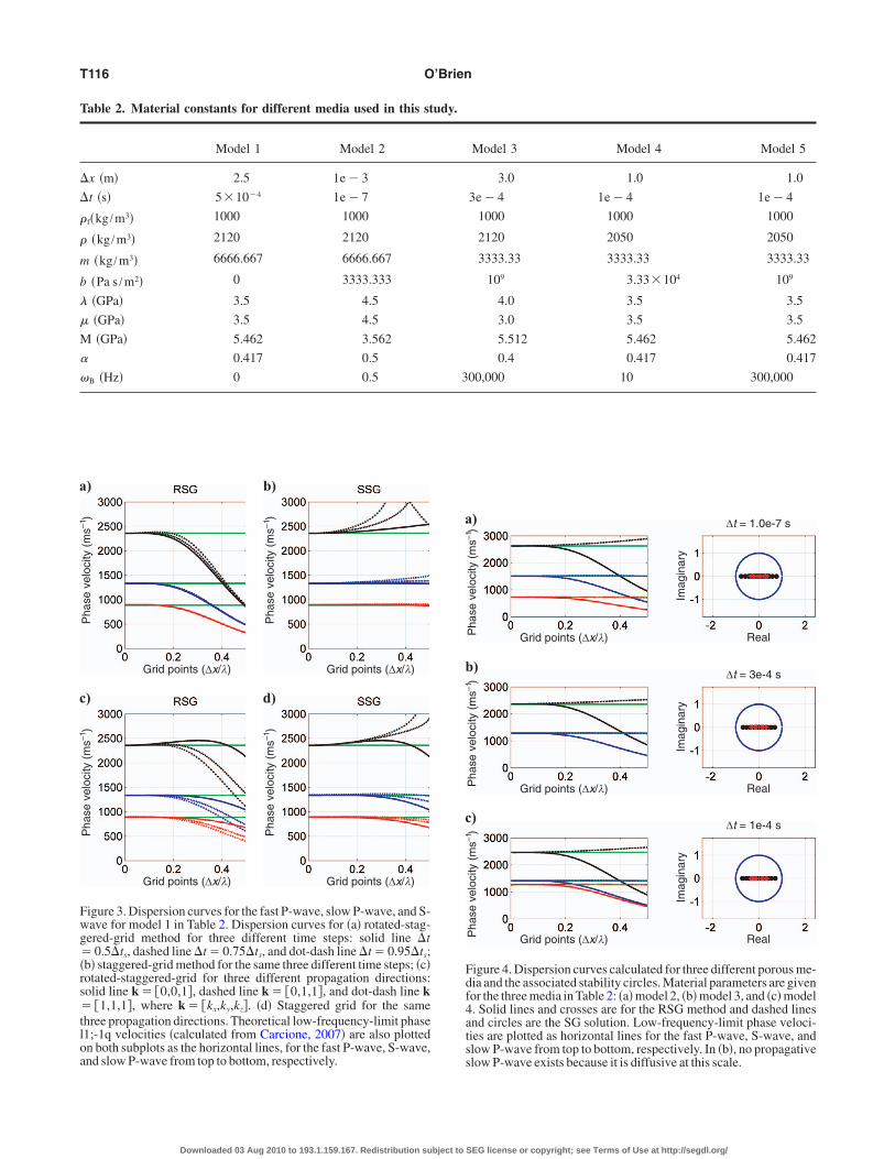
able 2. Material constants for different media used in this study.

Model 1 Model 2 Model 3 Model 4 Model 5

x �m� 2.5 1e�3 3.0 1.0 1.0

t �s� 5�10�4 1e�7 3e�4 1e�4 1e�4

f�kg /m3� 1000 1000 1000 1000 1000

�kg /m3� 2120 2120 2120 2050 2050

�kg /m3� 6666.667 6666.667 3333.33 3333.33 3333.33

�Pa s /m2� 0 3333.333 109 3.33�104 109

�GPa� 3.5 4.5 4.0 3.5 3.5

�GPa� 3.5 4.5 3.0 3.5 3.5

�GPa� 5.462 3.562 5.512 5.462 5.462

0.417 0.5 0.4 0.417 0.417

B �Hz� 0 0.5 300,000 10 300,000

a

b

c

Fdf4ats

) b)

) d)

–1P

hase

velo

city

(ms

)

Grid points (∆x/λ)

–1P

hase

velo

city

(ms

)


–1P

hase

velo

city

(ms

)


–1P

hase

velo

city

(ms

)


igure 3. Dispersion curves for the fast P-wave, slow P-wave, and S-ave for model 1 in Table 2. Dispersion curves for �a� rotated-stag-ered-grid method for three different time steps: solid line �t

0.5�ts, dashed line �t�0.75�ts, and dot-dash line �t�0.95�ts;b� staggered-grid method for the same three different time steps; �c�otated-staggered-grid for three different propagation directions:olid line k� �0,0,1�, dashed line k� �0,1,1�, and dot-dash line k

�1,1,1�, where k� �kx,ky,kz�. �d� Staggered grid for the samehree propagation directions. Theoretical low-frequency-limit phase1;-1q velocities �calculated from Carcione, 2007� are also plottedn both subplots as the horizontal lines, for the fast P-wave, S-wave,nd slow P-wave from top to bottom, respectively.
s

)

)

)

–1P

hase

velo

city

(ms

)


∆t = 1.0e-7 s

Imag

inar

y

Real

–1P

hase

velo

city

(ms

)


∆t = 3e-4 sIm

agin

ary

Real

–1P

hase

velo

city

(ms

)


∆t = 1e-4 s

Imag

inar

y

Real

igure 4. Dispersion curves calculated for three different porous me-ia and the associated stability circles. Material parameters are givenor the three media in Table 2: �a� model 2, �b� model 3, and �c� model. Solid lines and crosses are for the RSG method and dashed linesnd circles are the SG solution. Low-frequency-limit phase veloci-ies are plotted as horizontal lines for the fast P-wave, S-wave, andlow P-wave from top to bottom, respectively. In �b�, no propagativelow P-wave exists because it is diffusive at this scale.


rdtVbiouvrtfo

6R

tNbtmittshfFaitS

a

FSgalaM2v��

a

Fanismtbeftaeu


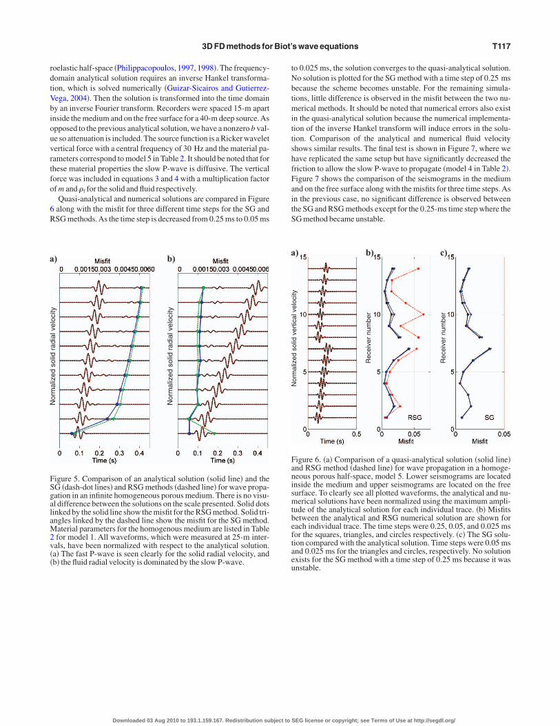
oelastic half-space �Philippacopoulos, 1997, 1998�. The frequency-omain analytical solution requires an inverse Hankel transforma-ion, which is solved numerically �Guizar-Sicairos and Gutierrez-ega, 2004�. Then the solution is transformed into the time domainy an inverse Fourier transform. Recorders were spaced 15-m apartnside the medium and on the free surface for a 40-m deep source.Aspposed to the previous analytical solution, we have a nonzero b val-e so attenuation is included. The source function is a Ricker waveletertical force with a central frequency of 30 Hz and the material pa-ameters correspond to model 5 in Table 2. It should be noted that forhese material properties the slow P-wave is diffusive. The verticalorce was included in equations 3 and 4 with a multiplication factorf m and �f for the solid and fluid respectively.Quasi-analytical and numerical solutions are compared in Figure

along with the misfit for three different time steps for the SG andSG methods.As the time step is decreased from 0.25 ms to 0.05 ms

Nor

mal

ized

solid

radi

alve

loci

ty

Nor

mal

ized

solid

radi

alve

loci

ty

) b)

igure 5. Comparison of an analytical solution �solid line� and theG �dash-dot lines� and RSG methods �dashed line� for wave propa-ation in an infinite homogeneous porous medium. There is no visu-l difference between the solutions on the scale presented. Solid dotsinked by the solid line show the misfit for the RSG method. Solid tri-ngles linked by the dashed line show the misfit for the SG method.aterial parameters for the homogenous medium are listed in Tablefor model 1. All waveforms, which were measured at 25-m inter-als, have been normalized with respect to the analytical solution.a� The fast P-wave is seen clearly for the solid radial velocity, andb� the fluid radial velocity is dominated by the slow P-wave.


o 0.025 ms, the solution converges to the quasi-analytical solution.o solution is plotted for the SG method with a time step of 0.25 msecause the scheme becomes unstable. For the remaining simula-ions, little difference is observed in the misfit between the two nu-

erical methods. It should be noted that numerical errors also existn the quasi-analytical solution because the numerical implementa-ion of the inverse Hankel transform will induce errors in the solu-ion. Comparison of the analytical and numerical fluid velocityhows similar results. The final test is shown in Figure 7, where weave replicated the same setup but have significantly decreased theriction to allow the slow P-wave to propagate �model 4 in Table 2�.igure 7 shows the comparison of the seismograms in the mediumnd on the free surface along with the misfits for three time steps. Asn the previous case, no significant difference is observed betweenhe SG and RSG methods except for the 0.25-ms time step where theG method became unstable.

Nor

mal

ized

solid

vert

ical

velo

city

Rec

eive

rnu

mbe

r

Rec

eive

rnu

mbe

r

) b) c)

igure 6. �a� Comparison of a quasi-analytical solution �solid line�nd RSG method �dashed line� for wave propagation in a homoge-eous porous half-space, model 5. Lower seismograms are locatednside the medium and upper seismograms are located on the freeurface. To clearly see all plotted waveforms, the analytical and nu-erical solutions have been normalized using the maximum ampli-

ude of the analytical solution for each individual trace. �b� Misfitsetween the analytical and RSG numerical solution are shown forach individual trace. The time steps were 0.25, 0.05, and 0.025 msor the squares, triangles, and circles respectively. �c� The SG solu-ion compared with the analytical solution. Time steps were 0.05 msnd 0.025 ms for the triangles and circles, respectively. No solutionxists for the SG method with a time step of 0.25 ms because it wasnstable.


tlBsawcitDawaeolbaasvsl

ssscFtbdtcrmdde

tsSkpft

a

T�

a

Fanisnpbetc0is

T118 O’Brien

CONCLUSIONS

We have implemented fourth-order in space and second-order inime staggered-grid and rotated-staggered-grid methods for the so-ution of Biot’s equation for wave propagation in a porous medium.iot equations are stiff and care must be taken when choosing the

cale of the problem because the Biot slow wave behaves diffusivelyt low frequency and becomes propagative at high frequencies.Also,ithout correcting for the viscous boundary layer at high frequen-

ies, the method should be restricted to the low-frequency regime,.e., ��B. The exact 3D numerical dispersion and stability condi-ions of the methods were derived using a von Neumann analysis.etermination of the required time step depends on the evaluation ofdeterminant of a 6�6 matrix. This matrix depends in a nontrivialay on the spatial grid step, the time step, and material parameters,

s well as the wavenumber. This prohibits the derivation of a simplexpression for the stability condition and dispersion curves. The usef a 1D approximate stability condition is not advised as the SG vio-ates it for specific material properties. The numerical methods haveeen verified against an analytical solution for an isotropic source inhomogeneous porous medium. In both methods, we have includedfree-surface boundary condition and compared our numerical re-

ults with a quasi-analytical solution. We show that the method pro-ides a good solution for wave propagation in a poroelastic half-pace. The free-surface boundary condition represents one of theargest material contrasts in any geological formation, and thus the

Nor

mal

ized

solid

vert

ical

velo

city

Rec

eive

rnu

mbe

r

Rec

eive

rnu

mbe

r

) b) c)

igure 7. �a� Comparison of a quasi-analytical solution �solid line�nd RSG method �dashed line� for wave propagation in a homoge-eous porous half-space, model 4. Lower seismograms are locatednside the medium and upper seismograms are located on the freeurface. To clearly see all the plotted waveforms, the analytical andumerical solutions have been normalized using the maximum am-litude of the analytical solution for each individual trace. �b� Misfitsetween the analytical and RSG numerical solution are shown forach individual trace. Time steps were 0.25, 0.05, and 0.025 ms forhe squares, triangles, and circles, respectively. �c� The SG solutionompared with the analytical solution. Time steps were 0.05 and.025 ms for the triangles and circles, respectively. No solution ex-sts for the SG method with a time step of 0.25 ms because it was un-table.


chemes are applicable to high medium contrasts once sufficientlymall spatial and temporal scales are selected. The RSG methodtays stable for a larger time step than the SG method, which reducesomputational time but comes at the cost of a reduction in accuracy.or sufficiently small time steps, no discernable difference between

he methods is observed for the examples illustrated here. It shoulde noted that accuracy of the methods depends on the propagationistance, temporal grid step, spatial grid step, and material proper-ies. Therefore, misfit errors calculated for the models used hereould increase or decrease equally depending on the computationalesources and model properties. Selection of an appropriate scale toinimize errors can be determined from the exact 3D stability con-

itions and dispersion curves. However, in seismology, the lack ofetailed velocity models usually would be responsible for the largestrror associated with computational wave propagation.

ACKNOWLEDGMENTS

The author wishes to acknowledge that this work was funded byhe Ireland Department of Communications, Energy and Natural Re-ources under the National Geoscience Programme 2007-2013. TheFI/HEA Irish Centre for High-End Computing �ICHEC� is ac-nowledged for the provision of computational facilities and sup-ort. The author would like to thank Chris Bean and Louis De Barrosor discussions. Comments and suggestions from four reviewers andhe associate editor greatly improved the original manuscript.

APPENDIX A

The staggered-grid first and second time and spatial derivativesre given by

� �u

�t�t

�Dtu�ut�∆t/2�ut�∆t/2

∆t, �A-1�

� �2u

�t2�t

�Dttu�ut�∆t�2ut�ut�∆t

∆t2, �A-2�

�u

�x� �Dxu�x,y,z��x��x/2,y,z��

c1

�x�u�x��x,y,z��u�x,y,z�

�c2

�x�u�x�2�x,y,z��u�x��x,y,z�� . �A-3�

he other derivative directions are calculated in a similar manner tou/�x. The RSG spatial derivatives are given by

�u

�x� �Dxu�x,y,z��x��x/2,y��x/2,z��x/2�

�1

4�x�c1�u�x��x,y,z��u�x��x,y,z��x��u�x

��x,y��x,z��u�x��x,y��x,z��x�

�u�x,y,z��u�x,y��x,z��u�x,y��x,z��x�

�u�x,y,z��x��c2�u�x�2�x,y��x,z��x�

�u�x�2�x,y�2�x,z��x��u�x�2�x,y��x,z


C1a

B

—

—

B

C

C

D

D

E

G

M

M

P

—

P

R

S

S

S

S

V

W


�2�x��u�x�2�x,y�2�x,z�2�x��u�x

��x,y��x,z��x��u�x��x,y�2�x,z��x�

�u�x��x,y��x,z�2�x��u�x��x,y�2�x,z

�2�x��, �A-4�

�u

�y� �Dyu�x,y,z��x��x/2,y��x/2,z��x/2�

�1

4�x�c1��u�x��x,y,z��u�x��x,y,z��x��u�x

��x,y��x,z��u�x��x,y��x,z��x�


�u�x,y,z��x��c2��u�x�2�x,y��x,z��x�

�u�x�2�x,y�2�x,z��x��u�x�2�x,y��x,z

�2�x��u�x�2�x,y�2�x,z�2�x��u�x

��x,y��x,z��x��u�x��x,y�2�x,z��x�

�u�x��x,y��x,z�2�x��u�x��x,y�2�x,z

�2�x��, �A-5�

�u

�x� �Dzu�x,y,z��x��x/2,y��x/2,z��x/2�

�1

4�x�c1��u�x��x,y,z��u�x��x,y,z��x��u�x

��x,y��x,z��u�x��x,y��x,z��x�


�u�x,y,z��x��c2��u�x�2�x,y��x,z��x�

�u�x�2�x,y�2�x,z��x��u�x�2�x,y��x,z

�2�x��u�x�2�x,y�2�x,z�2�x��u�x

��x,y��x,z��x��u�x��x,y�2�x,z��x�

�u�x��x,y��x,z�2�x��u�x��x,y�2�x,z

�2�x�� . �A-6�

onstants c1 and c2 are 9 /8 and �1 /24, respectively �Dablain,986�. Material variables aij, bij, and cij in matrix Q in equation 16re given by

a11�m� �� f2, �A-7�

b11��2m�� f�M �m�, �A-8�

c11��m�, �A-9�

a21��m��m�� f�M, �A-10�

a41�� fb, �A-11�


a51�b41��m�M �� fM, �A-12�

a14�2� f�� f��M, �A-13�

b14�� f�, �A-14�

a24�� f�� f��M, �A-15�

c44�a45�� f�M ��M . �A-16�

REFERENCES

iot, M. A., 1956a, Theory of propagation of elastic waves in a fluid-saturat-ed porous solid. I. Low-frequency range: Journal of the Acoustic SocietyofAmerica, 28, 168–178.—–, 1956b, Theory of propagation of elastic waves in a fluid-saturated po-rous solid. II. Higher-frequency range: Journal of the Acoustic Society ofAmerica, 28, 179–191.—–, 1962, Mechanics of deformation and acoustic propagation in porousmedia: Journal ofApplied Physics, 33, 1482–1498.

ohlen, T., 2002, Parallel 3-D viscoelastic finite difference seismic model-ling: Computers & Geosciences, 28, 887–899.

arcione, J. M., 2007, Wave fields in real media, second edition: Wave propa-gation in anisotropic, anelastic, porous and electromagnetic media:Elsevier.

arcione, J. M., and G. Quiroga-Goode, 1995, Some aspects of the physics ofand numerical modelling of Biot compressional waves: Journal of Com-putationalAcoustics, 4, 261–280.

ablain, M. A., 1986, The application of high-order differencing to the scalarwave equation: Geophysics, 51, 54–66.

ai, N., A. Vafidis, and E. R. Kanasewich, 1995, Wave propagation in hetero-geneous, porous media: A velocity-stress, finite difference method: Geo-physics, 60, 327–340.

mmerich, H., and M. Korn, 1987, Incorporation of attenuation into time-do-main computations of seismic wave fields: Geophysics, 52, 1252–1264.

uizar-Sicairos, M., and J. C. Gutierrez-Vega, 2004, Computation of quasi-discrete Hankel transforms of integer order for propagating optical wavefields: Journal of the Optical Society ofAmericaA, 21, 53–58.asson, Y. J., S. R. Pride, and K. T. Nihei, 2006, Finite difference modelingof Biot’s poroelastic equations at seismic frequencies, Journal of Geo-physical Research, 111, B10305, , doi: 10.1029/2006JB004366.oczo, P., J. Kristek, V. Varycuk, R. J. Archuleta, and L. Halada, 2002, 3Dheterogeneous staggered-grid finite-difference modeling of seismic mo-tion with volume harmonic and arithmetic averaging of elastic moduli anddensities: Bulletin of the Seismological Society of America, 92, 3042–3066.

hilippacopoulos, A. J., 1997, Buried point source in a poroelastic half-space: Journal of Engineering Mechanics, 123, 860–869.—–, 1998, Spectral Green’s dyadic for point sources in poroelastic media:Journal of Engineering Mechanics, 124, 24–31.

ress, W. H., S. A. Teukolsky, W. T. Vetterling, and B. Flannery, 2007, Nu-merical recipes, third edition: Cambridge University Press.

obertsson, J. O. A., J. O. Blanch, and W. W. Symes, 1994, Viscoelastic fi-nite-difference modeling: Geophysics, 59, 1444–1456.

aenger, E., T. Bohlen, 2004, Finite-difference modeling of viscoelastic andanisotropic wave propagation using the rotated staggered grid: Geophys-ics, 69, 583–591.

aenger, E. H., R. Ciz, O. S. Krüger, S. M. Schmalholz, B. Gurevich, and S.A. Shapiro, 2007, Finite-difference modeling of wave propagation on mi-croscale: A snapshot of the work in progress: Geophysics, 72, no. 5,SM293–SM300.

aenger, E. H., N. Gold, and S. Shapiro, 2000, Modelling the propagation ofelastic waves using a modified finite-difference grid: Wave Motion, 31,77–92.

heen, D., K. Tuncay, C. Baag, and P. J. Ortoleva, 2006, Parallel implemen-tation of a velocity-stress staggered-grid finite-difference method for 2-Dporoelastic wave propagation: Computers & Geosciences, 32, 1182–1191.

irieux, J., 1986, P-SV wave propagation in heterogeneous media: Velocity-stress finite-difference method: Geophysics, 51, 889–901.enzlau, F., and T. M. Müller, 2009, Finite-difference modeling of wavepropagation and diffusion in poroelastic media: Geophysics, 74, no. 4,T55–T66.


3d rotated and standard staggered finite-difference solutions to biot’s

Documents