3d reconstruction of environments for tele …yiannis/publications/aiaa06.pdf · american institute...

American Institute of Aeronautics and Astronautics

1

3D Reconstruction of Environments for Tele-Operation of Planetary Rover

Joseph Nsasi Bakambu, Sebastien Gemme, Pierre Allard, Tom Lamarche, Ioannis Rekleitis and Erik Dupius Canadian Space Agency, Saint-Hubert, Québec, Canada J3Y 8Y9

In this paper we consider the problem of constructing a 3D environment model for the tele-operation of a planetary rover. We presented our approach to 3D environment reconstruction from large sparse range data sets. In space robotics applications, an accurate and up-to-date model of the environment is very important for a variety of reasons. In particular, the model can be used for safe tele-operation, path planning and mapping points of interest. We propose an on-line reconstruction of the environment using data provided by an on-board high resolution and accurate 3D range sensor (LIDAR). Our approach is based on on-line acquisition of range scans from different view-points with overlapping regions, merge them together into a single point cloud, and then fit an irregular triangular mesh on the merged data. The experimental results demonstrate the effectiveness of our approach in localization, path planning and execution scenario on the Mars Yard located at the Canadian Space Agency.

I. Introduction HE recent success of the Mars Exploration Rovers “Spirit” and “Opportunity” has demonstrated the important benefits that mobility adds to landed planetary exploration missions. The recent announcement by NASA to

increase its activities in planetary exploration (via Moon and Mars missions) and the ESA Aurora program will certainly result in an increase in the number of robotic vehicles roaming on the surface of other planets. The current state-of-the-art in control of planetary rovers requires intensive human involvement throughout the planning portion of the operations. Unless the terrain is relatively easy to navigate, rovers are typically limited to traverses on the order of a few tens of meters. Recently, the Mars Exploration Rovers “Spirit” and “Opportunity” have managed to conduct traverses on the order of 100 meters per day.

To increase the science return, future planetary missions will undoubtedly require the ability to traverse even longer distances. Given the long communication delays and narrow communication windows of opportunity, it is impossible for Earth-based operators to drive Mars rovers in an interactive manner. Furthermore, over long traverses, the detailed geometry of the environment cannot be known a priori. In this context, planetary rovers will require the ability to navigate autonomously over long distances.

One of the key technologies that will be required is the ability to sense and model the 3D environment in which the rover has to navigate. For long-range navigation, the ability to register maps and stitch them together is also required. Some of the challenges specific to our application include the fact that most terrain scans are taken from a shallow grazing angle, giving point clouds of variable resolution and containing sparse data as a result of occlusions. In addition, the global localization may require the registration of maps with different resolutions taken from different viewpoints.

Several methods already exist to reconstruct surfaces from sets of points. Of particular interest are free-form surfaces, which have well defined normal vectors everywhere (with a few exceptions). A common approach is using NURBS (Non-Uniform Rational B-Spline), but sometimes NURBS-surfaces are impossible to accurately fit on point clouds. Polygonal meshes continue today to be the most popular choices; for a more extensive review please refer to Campbell and Flynn [4]. Hoppe et. al. [10] proposed an algorithm that is robust to undersampling and can handle large volumes of data. The main idea is to divide the space into cubes and retrieve the crossing points of the surface with the cubes. By collecting these intersection points one can rebuild the mesh. Following that, a mesh simplification is applied. Finally, a subdivision surface is generated. The drawback of those approaches is the fact that the original surface's points do not represent the final surface.

Another approach to free-form surface generation is based on the Delaunay triangulation [8]. The original approach was appropriate for small data sets and uniform sampling. Dey et al. [12] have extended the previous method to deal with undersampling. Further variations of these algorithms has been developed in order to address

T


2

the problem of large data set using a Delaunay based method; e.g. SUPERCOCONE by Dey et. al. [13]. Nebot et al. [11] partitioned the surface into a set of connected local triangular regions combined with occupancy grid maps. Torres and Dudek [9] combine information from intensity and range images in order to compensate for sparse data, and fill in any gaps.

The next section describes our approach to 3D surface reconstruction from large sparse range data sets and discusses how constructing a reliable model can significantly increase the on-board autonomy. Our approach is based on acquiring range scans from different view-points with overlapping regions, merging them together into a single data set, and fitting a triangular mesh on the merged data points. The triangulation data structure selected for the terrain representation provides valuable information in the form of the connectivity graph that allows for efficient retrieval of the adjacent triangles from the current triangle. Section 3 presents how this valuable information is enhanced to generate a safe-trajectory from a given start position to the goal position. Section 4, describes the rover guidance that can keep the robot precisely on the planned trajectory. Finally, we provide experimental results performed in a challenging terrain of the Mars Yard located at the Canadian Space Agency. This Mars Yard simulates the topography found in typical Mars landscapes.

II. Environment Modeling Complete 3D reconstruction of a free-form surface requires

acquisition of data from multiple viewpoints in order to compensate for the limitations of the field of view and for self-occlusions. We used an ILRIS-3D LIght Detection And Ranging (LIDAR) sensor (see Figure 1) for scanning views of a 3D surface to obtain 2.5D point clouds. The reconstruction of the environment is performed in two steps. The first step consists of the assembly of the different views by estimating the rigid transformation between the poses from where each view was taken. The second step is the environment reconstruction, achieved by fitting an irregular triangular mesh on the point cloud that combines the data from all views

Two problems have to be mentioned in this application. First, is the challenge of dealing with large data sets, as each LIDAR scan has about 500K 3D points, and the combination of multiple scans is required. Therefore, the data sets can easily grow to millions of points. Any approach used has to be robust for high volume of data. The second challenge is the sparsity of the point cloud and the non-uniform density of scans as it can be seen in Figure 2.

A. Assembly of the Different Scans In this step, different scans are registered in

a common coordinate system. Since the coordinates of the viewpoint may not be available or may be inaccurate, the original Iterative Closest Points (ICP) by Besl and McKay [1] may not converge to the global minimum. Thus, to assemble all views in the same coordinate frame, we used a variant of ICP [7], which differs from the original ICP by searching for the closest point under a constraint of similarity in geometric primitives. The geometric primitives used in [7] are the normal vector and the change of geometric curvature. The change of geometric curvature represents how much the surface formed by a point and its neighbors deviates from the tangential plane [2], and is invariant to the 3D rigid motion.

Figure 1. LIDAR Sensor from Optech

2 1 3

Figure 2. The three scans (scan 1, scan 2, scan 3) to be assembled.


3

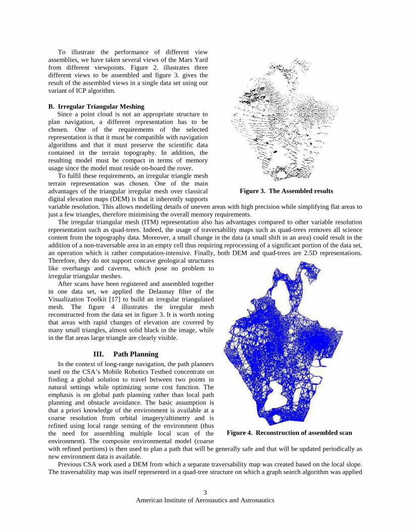
To illustrate the performance of different view assemblies, we have taken several views of the Mars Yard from different viewpoints. Figure 2. illustrates three different views to be assembled and figure 3. gives the result of the assembled views in a single data set using our variant of ICP algorithm.

B. Irregular Triangular Meshing Since a point cloud is not an appropriate structure to

plan navigation, a different representation has to be chosen. One of the requirements of the selected representation is that it must be compatible with navigation algorithms and that it must preserve the scientific data contained in the terrain topography. In addition, the resulting model must be compact in terms of memory usage since the model must reside on-board the rover.

To fulfil these requirements, an irregular triangle mesh terrain representation was chosen. One of the main advantages of the triangular irregular mesh over classical digital elevation maps (DEM) is that it inherently supports variable resolution. This allows modelling details of uneven areas with high precision while simplifying flat areas to just a few triangles, therefore minimising the overall memory requirements.

The irregular triangular mesh (ITM) representation also has advantages compared to other variable resolution representation such as quad-trees. Indeed, the usage of traversability maps such as quad-trees removes all science content from the topography data. Moreover, a small change in the data (a small shift in an area) could result in the addition of a non-traversable area in an empty cell thus requiring reprocessing of a significant portion of the data set, an operation which is rather computation-intensive. Finally, both DEM and quad-trees are 2.5D representations. Therefore, they do not support concave geological structures like overhangs and caverns, which pose no problem to irregular triangular meshes.

After scans have been registered and assembled together in one data set, we applied the Delaunay filter of the Visualization Toolkit [17] to build an irregular triangulated mesh. The figure 4 illustrates the irregular mesh reconstructed from the data set in figure 3. It is worth noting that areas with rapid changes of elevation are covered by many small triangles, almost solid black in the image, while in the flat areas large triangle are clearly visible.

III. Path Planning In the context of long-range navigation, the path planners

used on the CSA’s Mobile Robotics Testbed concentrate on finding a global solution to travel between two points in natural settings while optimizing some cost function. The emphasis is on global path planning rather than local path planning and obstacle avoidance. The basic assumption is that a priori knowledge of the environment is available at a coarse resolution from orbital imagery/altimetry and is refined using local range sensing of the environment (thus the need for assembling multiple local scan of the environment). The composite environmental model (coarse with refined portions) is then used to plan a path that will be generally safe and that will be updated periodically as new environment data is available.

Previous CSA work used a DEM from which a separate traversability map was created based on the local slope. The traversability map was itself represented in a quad-tree structure on which a graph search algorithm was applied

Figure 3. The Assembled results

Figure 4. Reconstruction of assembled scan


4

to find a safe path. While this approach worked, it required a separate structure for the terrain data and traversability map, which forced the update of the traversability map and the quad-tree structure when the DEM was modified.

An other advantage of ITM is their built-in ability to support non-uniform resolution within the same data set as well as zones of missing data. Both of these features are useful when dealing with point clouds generated with a rover mounted LIDAR that provides data resolution that varies with distance and that contains zones missing data in shadowed areas.

The use of ITM to represent terrain data allows us to integrate the terrain representation with the path planning easily. This is done using an undirected weighted graph representing the triangles connectivity. The graph is created where the triangles are the vertices of the graph and a triangle's connectivity to its neighbours are represented as edges. The JGraphT Java Library [18] has been used to implement the graph structure and functions.

The edge weight or cost is defined by providing a function that yields a cost based on the distance between the vertices, slope of the edge, slope of the triangles, mean altitude, or a combination of these to yield the cost associated with moving from one triangle to another. The cost function is associated to the edges at the graph creation, but the actual cost is computed only upon request, when the graph is searched.

Once the graph is constructed, a path between the current rover location and a destination can be planned. The process involves four steps:

1. Finding the two triangles where the current location and the destination lie. 2. Applying the Dijkstra's shortest path search algorithm [18] to find the "cheapest" path. 3. Creating a list of waypoints based on the path found. 4. Generating a simplified trajectory from the list of waypoints. Applying the Dijkstra's shortest path algorithm on the triangle connectivity graph from the current location to the

destination triangles produces a list of edges along the path. This list is used to create a list of the triangles to be traversed. Finding the center of each of the triangles making the path yields a list of waypoints.

Figure 6. Trajectory after simplification

Figure 5. Trajectory generated using waypoint list

Figure 7. Trajectory minimizing slope and distance

Figure 8. Trajectory favoring high ground


5

The trajectory defined by the waypoints list has often a "saw tooth" look, which makes it difficult to follow for the robot guidance. In order to alleviate this problem, the waypoint list is processed in order to remove unnecessary waypoints while maintaining the resulting trajectory on safe ground. Figure 5 and Figure 6 show the effect of the trajectory simplification.

Various cost functions have been tested with the path planner. For example, Figure 7 shows the result for planning a path from location (15.0, 5.0) to (80.0, 100.0) (in meters) using a cost function that takes into account distance and slope. Figure 8 shows a trajectory generated using a variation on the previous cost function. This function favours high grounds over low grounds and could be used to improve a robot's view of the terrain

IV. Guidance The usage of a scanning lidar for terrain sensing results in a concept of operation slightly different from the more

common schemes using stereo pairs. Indeed the scanning lidar used on the CSA’s Mobile Robotics Test-bed typically takes on the order of one or two minutes to perform a terrain scan but it has a sensing range of over a kilometer. As a result, the terrain is not sensed continuously. It is rather imaged using snapshots taken at discrete intervals. Obviously, since the lidar is located near ground level, the effective range of the measurements is typically not on the order of kilometers but of a few tens of meters. Consequently, the rover has the ability to plan path segments on the order of 20 to 30 meters and does not rely on environment sensing while moving along these path segments. It has, therefore, been necessary to develop a guidance algorithm that can keep the robot precisely on the planned trajectory. The proposed rover guidance has two mains parts: localization and autonomous motion control.

A. Localization The first step to ensure that the robot does not deviate from the planned trajectory is to provide accurate

knowledge of its position. In our system, this task is accomplished by two localization methods. The first method, 3D odometry, continuously estimates the pose of the rover while the second method, scans/maps matching, is used to estimate the initial global pose of the rover and also to periodically correct the 3D accumulated error.

1. 3D Odometry based Localization

Our 3D odometry is a Kalman filter based fusion of odometry from the rover encoders with the orientation in SO(3) from an Inertial Measurement Unit (IMU), and the absolute heading from a digital compass TCM2. The compass is activated only when the robot stops (e.g. for taking new scan) because the compass data is not reliable when the robot motors are running due to the electromagnetic interference. In Mars, a sun sensor would replace this sensor. More details on the performances and the experimental evaluation of our 3D odometry can be find in Dupuis et al.[6].

2. Scans/Maps Matching based 3D Localization

Two cases can be considered: with and without knowledge of the a priori estimation of the viewpoint. In the first case (in our system, the viewpoint is provided by the 3D odometry), the variant of ICP presented in section 2.1 is good enough to register scans and provides a more accurate viewpoint estimation, as illustrated in Figure 9. In this figure, scan 1 and scan 2 (from Figure 2) are registered.

In the second case, without any knowledge of a priori of the viewpoint, features that are independent to rigid motion need to be extracted. Those features are for example, geometric histogram, harmonic shape image, surface signature, footprint point signature, point fingerprint, spherical attribute image, and spin-image. More exhaustive list and details of invariant features is given in [3]. Feature-based approaches drawbacks are mainly that they cannot solve the problem in which the 3D data sets doest not contain salient local features and high computation time for extracting and organizing those invariant features. Their advantage is that they do not require an initial estimate of the viewpoint.

Figure 9. Registration of scans: scan 1 (left) and

scan 2 (right).


6

CSA is currently investigating three approaches for scan matching with no initial estimate of the viewpoint: harmonic shape image [15], point fingerprint [21] and spin-image [5] matching. The results presented in this paper are based on Point fingerprint matching enhanced with Random Sample Consensus Algorithm based Data-Aligned Rigidity-Constrained (POINT-FINGERPRINT_RANSAC_DARCES) [20].

B. Point Fingerprint matching Matching takes place by having four separate steps: first step is to select points of interest in the scene and the

model. Scene being the scan taken from the sensor and model being the global map of the environment. Interest points are extracted using the curvature change method [2]. Once the points of interest are selected, a fingerprint representation is generated for each of them. To generate a fingerprint representation of a point, one has to define a fixed number of geodesic circles. The radius of a circle is the geodesic distance from the interest points. Geodesic distance is an appropriate choice because it is less sensitive to mesh resolution and configuration since it is following the mesh's surface instead of the edge of the triangles (figure 10).

Once the geodesic circles generated, each point of the circles is projected on the tangent plane of the surface at

the interest points, i.e. the center. After projecting the circles' points on the tangent plane, a constant re-sampling of circles' points is performed. The result of the projection is presented in figure 11.

The fingerprints are compared using cross-correlation radius of the circles at each point of every circle in the fingerprint. More detailed information of this procedure is presented in [21].

Once the fingerprint matching is completed, many outliers are present but the size of data to be treated has been significantly reduced. Another method based on the RANSAC BASED DARCES [20] is then used as a final step. This method has been modified to use the reduced information set obtained from the fingerprint matching, which allows it to complete in acceptable time. It has proven to be a key element in the algorithm since it is filtering the outliers, thus providing the initial estimate of the rigid body transformation. The initial estimate is then passed to an ICP algorithm that results in a very precise registration. Figure 12 shows the final result of the global localization without a priori knowledge of the rigid-motion parameters.

Figure 10. Geodesic circles surrounding the

feature point.

Figure 11. Resulting fingerprint

Figure 12. Global localization: a scan of a resolution of 20cm is successfully registered in a

model of a resolution of 1m.


7

C. Motion controller The developed motion control is based on a discontinuous state feedback control law initially proposed by

Astolfi [19]. Experimental results in an outdoor 3D environment (Figure 15) demonstrate the robustness and the stability of the developed path-following approach. The Figure 13 and the Figure 14 illustrate an 8m by 8m square-shaped reference path following result. A part on the path was on a slope. The dashed line represents the planned trajectory that covers an 8m by 8m region. The solid line represents the actual robot positions in 3D. In the far edge along the x-axis the vertical difference between the solid line and the dashed line is due to the fact that the commanded trajectory does not take into account a rise in the physical terrain. During the autonomous motion

execution, artificial perturbations were induced twice as show in Figure 14. This figure shows that the rover can robustly, quickly and smoothly recover the path.

During our tests with and without perturbations, physical error at the end of the motion was always negligible (about few centimeters in position and few degrees in orientation) and it is essentially due to the wheels slippage and the gyroscope drift. For example, the errors of the test in Figure 13 were on the order of 15 centimeters in position and 3.3 degree in orientation for 32 meters trajectory. The physical error in position was measured by putting marks on the ground, while an onboard compass (in rest state) provided the orientation error.

Those results illustrate the precision and the performance of the proposed autonomous motion controller and the 3D odometry based localization.

V. EXPERIMENTAL RESULTS To evaluate the efficiency of the proposed 3D

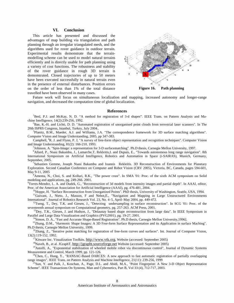
reconstruction of the environment approach, a global localization and path-planning scenario using the reconstructed model is tested in the Mars Yard (Figure 15). The mobile robot is placed some-where in the Mars Yard (at unknown position A) and asked to find a safe path up to a given global position of point B(see Figure 16). The unique a priori known information is a low (one meter) resolution map of the Mars Yard. The experimental results are shown in Figure 12 for the global localization illustration and in Figure 16 for the path planning. In Figure 12, first the rover takes a high-resolution scan and then uses the POINT-FINGER-PRINT-RANSAC Based DARCES algorithm to match it with a low-resolution model of Mars Yard without any knowledge of the position of the rover in the Mars Yard. The obtained result is the global position and orientation of the rover in Mars yard. This process takes approximately from 30 seconds to 2 minutes (Pentium 4, 1.8 GHz, which is acceptable for Mars exploration application since the rover has to do it only once to initialize the 3D odometry). In Figure 12, the registration results are: position of the rover (x=59.259, y=18.973, z=0.371) in meters and orientation of the rover (roll= -0.311, pitch= -0.633, yaw=-176.192) in degrees.

02

46

810

0

2

4

6

8

10-0.5

0

0.5

1

X (meters)

Guidance Results in 3D Terrain

Y (meters)

Z

Commanded TrajectoryActual Trajectory (3D Odometry)

Figure 13. Square-shaped path following with

artificially induced perturbations: 3D view.

-1 0 1 2 3 4 5 6 7 8 9-1

0

1

2

3

4

5

6

7

8

9

X (meters)

Y

2D projection of Guidance Results

Way pointsCommended TrajectoryActual Trajectory (3D Odometry)

Artificially induced pertubations

Figure 14. Square-shaped path following with artificially induced perturbations: 2D projection.

Figure 15. A view of the Mars Yard located at

Canadian Space Agency.


8

VI. Conclusion This article has presented and discussed the

advantages of map building via triangulation and path planning through an irregular triangulated mesh, and the algorithms used for rover guidance in outdoor terrain. Experimental results demonstrate that the terrain-modelling scheme can be used to model natural terrains efficiently and is directly usable for path planning using a variety of cost functions. The robustness and stability of the rover guidance in rough 3D terrain is demonstrated. Closed trajectories of up to 50 meters have been executed successfully in natural terrain even in the presence of external disturbances. Position errors on the order of less than 1% of the total distance travelled have been observed in many cases.

Future work will focus on simultaneous localization and mapping, increased autonomy and longer-range navigation, and decreased the computation time of global localization.

References 1Besl, P.J. and McKay, N. D. “A method for registration of 3-d shapes” . IEEE Trans. on Pattern Analysis and Ma-

chine Intelligence, 14(2):239-256, 1992. 2Bae, K.-H. and Lichti, D. D. "Automated registration of unorganised point clouds from terrestrial laser scanners". In The

20th ISPRS Congress, Istanbul, Turkey, July 2004.. 3Planitz, B.M., Maeder, A.J. and Williams, J.A. "The correspondence framework for 3D surface matching algorithms".

Computer Vision and Image Understanding, 2005, pp 347-383. Campbell, 4R. J. and Flynn, P. J, "A survey of free-form object representation and recognition techniques". Computer Vision

and Image Understranding, 81(2): 166-210, 1993. 5Johnson, A. "Spin-Image: a representation for 3-D surfacematching". Ph.D thesis, Carnegie Mellon University, 1997. 6Allard, P., Nsasi Bakambu, J., Lamarche,T, Rekleitis,I. and Dupuis, E., "Towards autonomous long range navigation". 8th

International Symposium on Artificial Intelligence, Robotics and Automation in Space (i-SAIRAS), Munich, Germany, September, 2005.

7Sebastien Gemme, Joseph Nsasi Bakambu and Ioannis Rekleitis. 3D Reconstruction of Environments for Planetary Exploration. Second Canadian Conference on Computer and Robot Vision (CRV 2005), Victoria, BC, Canada, pages 594-601, May 9-11, 2005

8Amenta, N., Choi, S. and Kolluri, R.K., "The power crust". In SMA '01: Proc. of the sixth ACM symposium on Solid modeling and applications, pg. 249-266. 2001. 9Torres-Mendez, L. A. and Dudek, G., "Reconstruction of 3d models from intensity images and partial depth". In AAAI, editor, Proc. of the American Association for Artificial Intelligence (AAAI), pg. 476-481, 2004.

10Hoppe, H. "Surface Reconstruction from Unorganized Points". PhD thesis, University of Washington, Seattle, USA, 1994. 11Guivant, J., Nieto, J., Masson, F and Nebot,E., "Navigation and Mapping in Large Unstructured Environments

International". Journal of Robotics Research Vol. 23, No. 4–5, April–May 2004, pp. 449-472. 12Tseng, T., Dey, T.K. and Giesen, J., "Detecting undersampling in surface reconstruction". In SCG '01: Proc. of the

seventeenth annual symposium on Computational geometry, pg. 257-263. ACM Press, 2001. 13Dey, T.K., Giesen, J. and Hudson, J., "Delaunay based shape reconstruction from large data". In IEEE Symposium in

Parallel and Large Data Visualization and Graphics (PVG2001), pg. 19-27, 2001. 14Simon, D. A., "Fast and Accurate Shape-Based Registration". Ph.D thesis, Carnegie Mellon University,1996]. 15Zhang, D.M., "Harmonic Shape Images: A 3D Free-form Surface Representation and its Application in surface Maching".

Ph.D thesis, Carnegie Mellon University, 1999. 16Zhang, Z., "Iterative point matching for registration of free-form curves and surfaces". Int. Journal of Computer Vision,

13(2):119-152, 1992. 17Kitware Inc. Visualization Toolkits. http://www.vtk.org, Website (accessed: September 2005) 18Naveh, B., et al. JGraphT, http://jgrapht.sourceforge.net Website (accessed: September 2005) 19Astolfi, A., "Exponential stabilization of wheeled mobile robot via discontinuous control", Journal of Dynamic Systems

Measurement and Control, March 1999, pp. 121-126. 20Chen, C., Hung, Y., "RANSAC-Based DARCES: A new approach to fast automatic registration of partially overlapping

range images". IEEE Trans. on Pattern Analysis and Machine Intelligence, 21(11): 239-256, 1999 21Sun, Y. and Paik, J., Koschan, A., Page, D.L. and Abidi, M.A., "Point Fingerprint: A New 3-D Object Representation

Scheme". IEEE Transactions On Systems, Man and Cybernetics, Part B, Vol 33 (4), 712-717, 2003.

B

A

Figure 16. Path planning

3d reconstruction of environments for tele …yiannis/publications/aiaa06.pdf · american institute...

Documents