3D Computer Vision

Prof. Didier Stricker

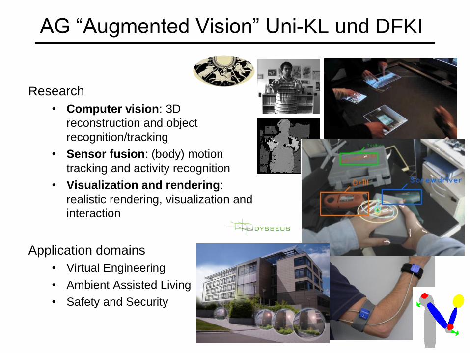
AG ―Augmented Vision‖ Uni-KL und DFKI

Research

• Computer vision: 3D

reconstruction and object

recognition/tracking

• Sensor fusion: (body) motion

tracking and activity recognition

• Visualization and rendering:

realistic rendering, visualization and

interaction

Application domains

• Virtual Engineering

• Ambient Assisted Living

• Safety and Security

3D Computer Vision:

• Lecture: Wednesday - 8:15 – 9:45

• Exercices: 1 hour per week

• SWS: 2V+1Ü

• Credit point: 4 LP

• Language: english

3D Computer Vision: lecture

• Topics: • Introduction: what is a camera?

• Camera model and camera calibration

• Fitting and parameter estimation

• Image point detection and point matching

• 2D-image transformation (mapping) and

panorama

• Two cameras: epipolar geometry and

triangulation

• Multiple views reconstruction

• Depth maps and multiple view stereo

reconstruction

• Structured light: laser, coded light

images

3D reconstruction

Camera pose

Texturing

3D Computer Vision: Exercices

• Homework assignments, consisting of

– theoretical part (questions) and

– practical part (Matlab implementation)

to be solved and handed in in groups of max. 3 students (by email)

• Accompanying supervised exercise sessions: two hours every two

weeks (discussion of last exercise, presentation/preparation of current

exercise)

• Room: probably 32/411 (computer pool) SCI account required

• Time: Monday, 17:00 to 19:00

• Starting 07.11.2011, possibly 21.11.2011

• Exam: Oral exam. In order to qualify, a minimum average score of

60% in the exercises is required.

• Next lecture (include exercices): 26th October– Introduction to

Matlab (Tobias Nöll, Johannes Köhler)

Contact

Prof. Didier Stricker

Tobias Nöll: Tobias.Noell@dfki.de

Johannes Köhler: Johannes.Koehler@dfki.de

Dr. Gabriele Bleser: Gabriele.Bleser@dfki.de

http://av.dfki.de -> Lectures

Example

Input images Structure From Motion

Multiple View Stereo

3D model

Today: The Camera

Overview

• The pinhole projection model • Qualitative properties

• Perspective projection matrix

• Cameras with lenses • Depth of focus

• Field of view

• Lens aberrations

• Digital cameras • Types of sensors

• Color

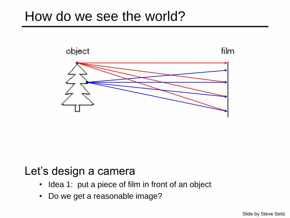
How do we see the world?

Let’s design a camera • Idea 1: put a piece of film in front of an object

• Do we get a reasonable image?

Slide by Steve Seitz

Pinhole camera

Add a barrier to block off most of the rays • This reduces blurring

• The opening known as the aperture

Slide by Steve Seitz

Pinhole camera model

Pinhole model: • Captures pencil of rays – all rays through a single point

• The point is called Center of Projection (focal point)

• The image is formed on the Image Plane

Slide by Steve Seitz

Point of observation

Figures © Stephen E. Palmer, 2002

Dimensionality Reduction Machine (3D to 2D)

3D world 2D image

What have we lost? • Angles

• Distances (lengths) Slide by A. Efros

Projection properties

• Many-to-one: any points along same ray map

to same point in image

• Points → points • But projection of points on focal plane is undefined

• Lines → lines (collinearity is preserved) • But line through focal point projects to a point

• Planes → planes (or half-planes) • But plane through focal point projects to line

Projection properties

• Parallel lines converge at a vanishing point • Each direction in space has its own vanishing point

• But parallels parallel to the image plane remain parallel

• All directions in the same plane have vanishing points on the

same line

How do we construct the vanishing point/line?

One-point perspective

Masaccio, Trinity, Santa

Maria Novella,

Florence, 1425-28

First consistent use of

perspective in

Western art?

Perspective distortion

• Problem for architectural photography:

converging verticals

Source: F. Durand

Perspective distortion

• What does a sphere project to?

Image source: F. Durand

Perspective distortion

• What does a sphere project to?

Perspective distortion

• The exterior columns appear bigger

• The distortion is not due to lens flaws

• Problem pointed out by Da Vinci

Slide by F. Durand

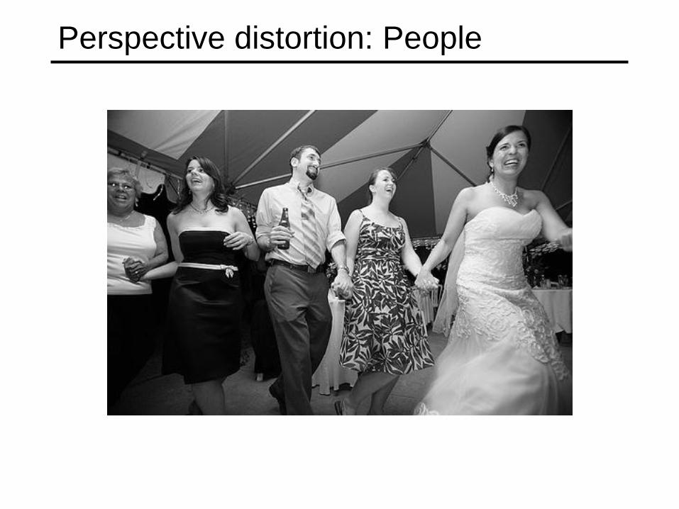
Perspective distortion: People

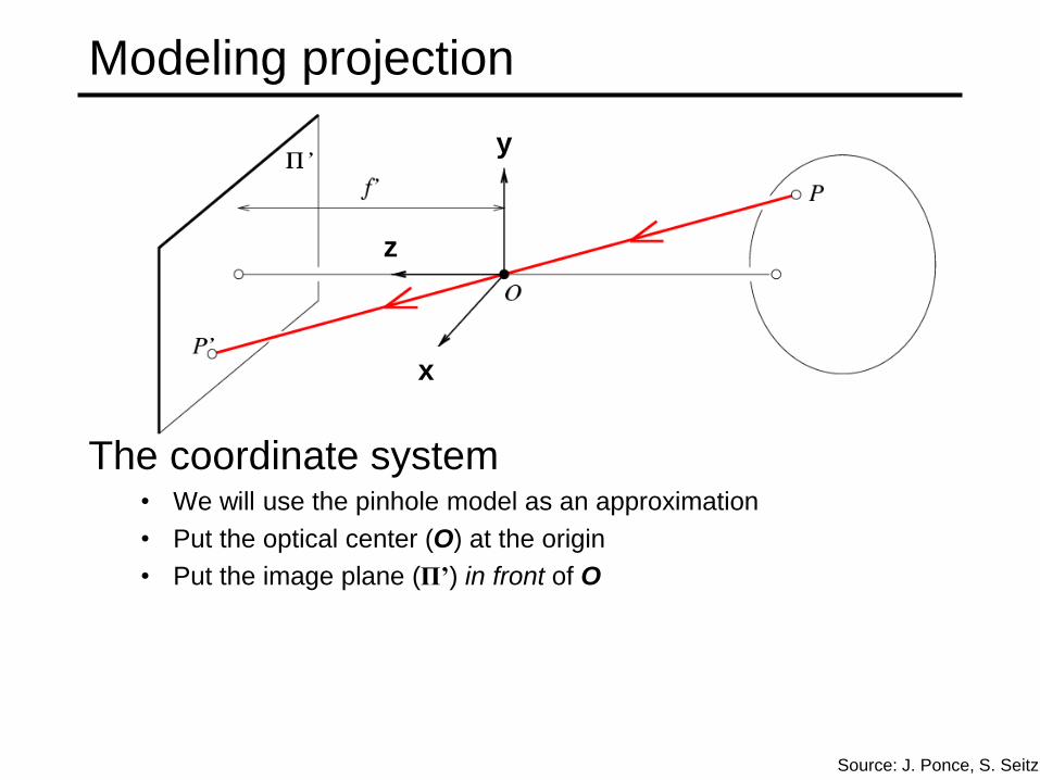
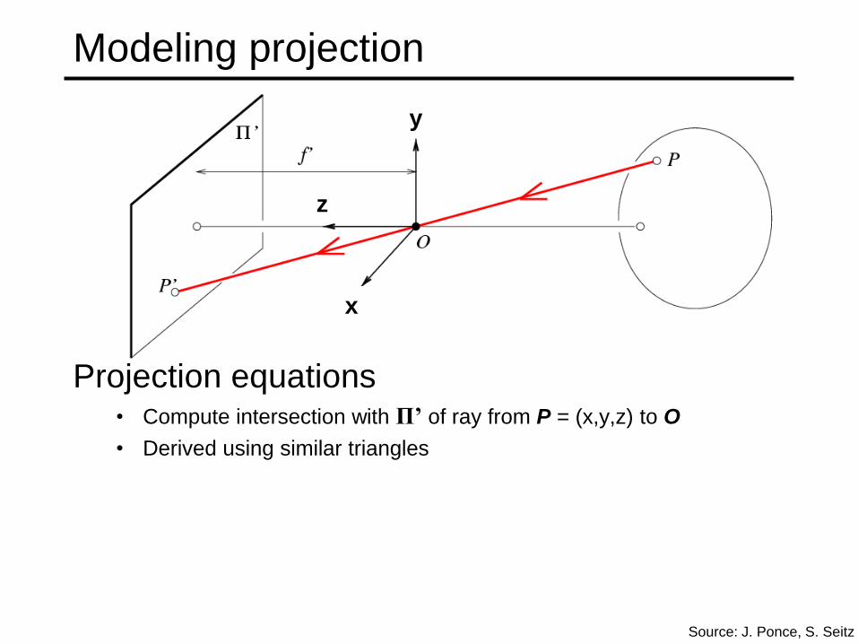
Modeling projection

The coordinate system • We will use the pinhole model as an approximation

• Put the optical center (O) at the origin

• Put the image plane (Π’) in front of O

x

y

z

Source: J. Ponce, S. Seitz

x

y

z

Modeling projection

Projection equations • Compute intersection with Π’ of ray from P = (x,y,z) to O

• Derived using similar triangles

)',','(),,( fz

yf

z

xfzyx

Source: J. Ponce, S. Seitz

• We get the projection by throwing out the last coordinate:

)','(),,(z

yf

z

xfzyx

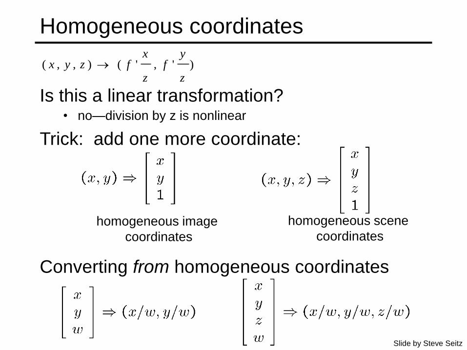
Homogeneous coordinates

Is this a linear transformation?

Trick: add one more coordinate:

homogeneous image

coordinates

homogeneous scene

coordinates

Converting from homogeneous coordinates

• no—division by z is nonlinear

Slide by Steve Seitz

)','(),,(z

yf

z

xfzyx

divide by the third

coordinate

Perspective Projection Matrix

Projection is a matrix multiplication using homogeneous

coordinates:

'/1

0'/100

0010

0001

fz

y

x

z

y

x

f

)','(z

yf

z

xf

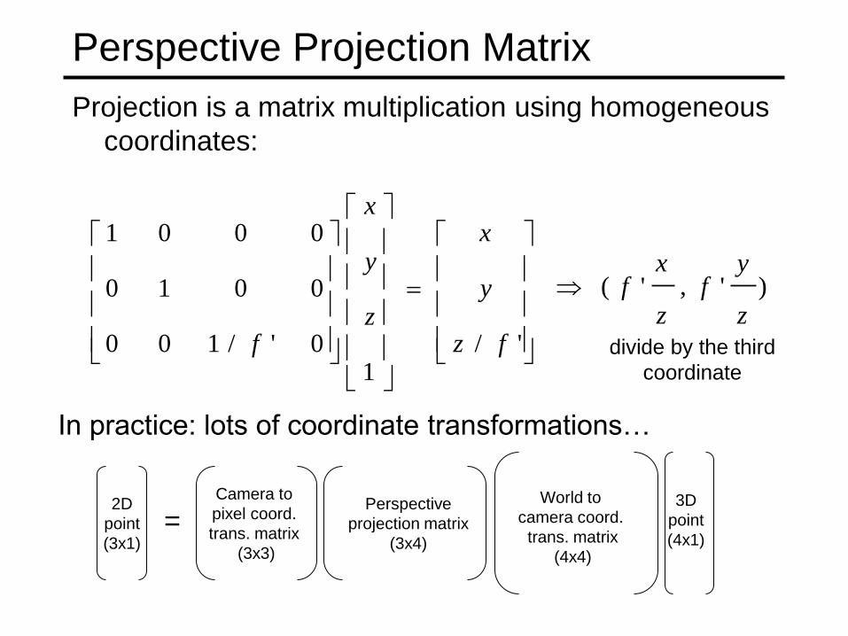
divide by the third

coordinate

Perspective Projection Matrix

Projection is a matrix multiplication using homogeneous

coordinates:

'/1

0'/100

0010

0001

fz

y

x

z

y

x

f

)','(z

yf

z

xf

In practice: lots of coordinate transformations…

World to

camera coord.

trans. matrix

(4x4)

Perspective

projection matrix

(3x4)

Camera to

pixel coord.

trans. matrix

(3x3)

= 2D

point

(3x1)

3D

point

(4x1)

Building a real camera

Camera Obscura

• Basic principle known to

Mozi (470-390 BCE),

Aristotle (384-322 BCE)

• Drawing aid for artists:

described by Leonardo

da Vinci (1452-1519)

Gemma Frisius, 1558

Source: A. Efros

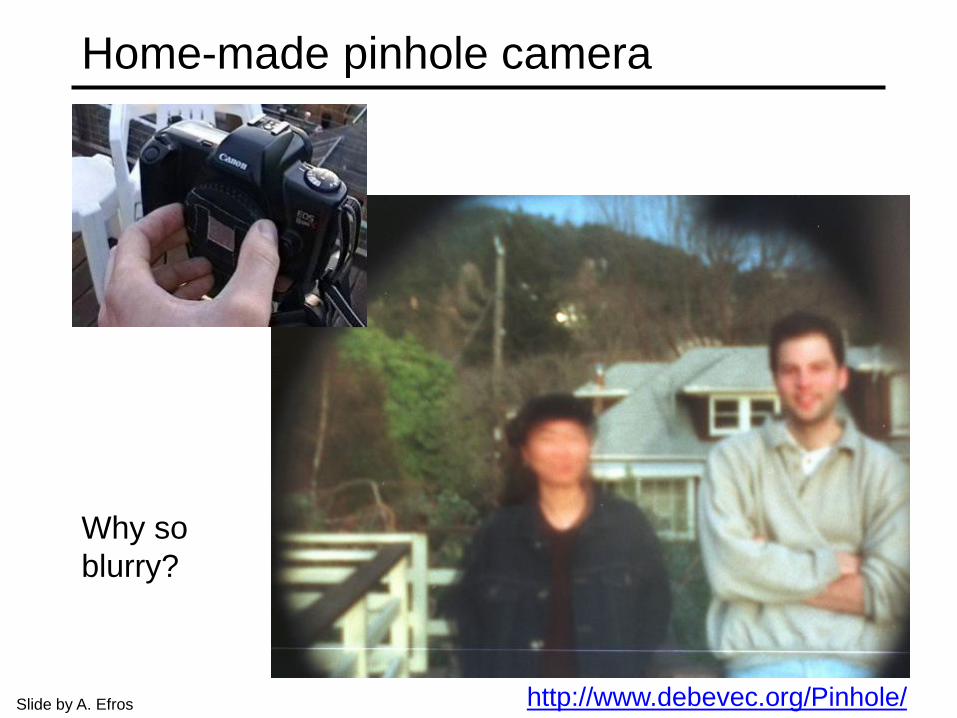
Home-made pinhole camera

http://www.debevec.org/Pinhole/

Why so

blurry?

Slide by A. Efros

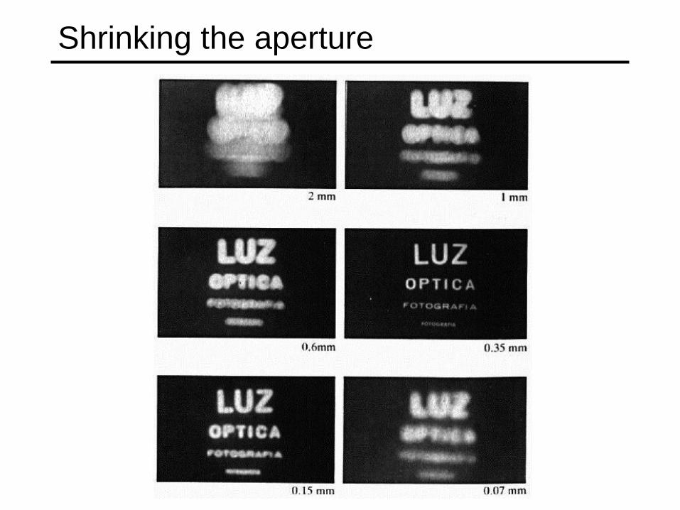
Shrinking the aperture

Why not make the aperture as small as possible? • Less light gets through

• Diffraction effects…

Slide by Steve Seitz

Shrinking the aperture

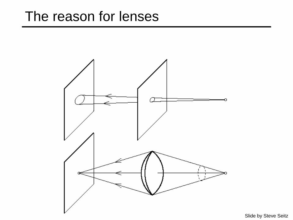
The reason for lenses

Slide by Steve Seitz

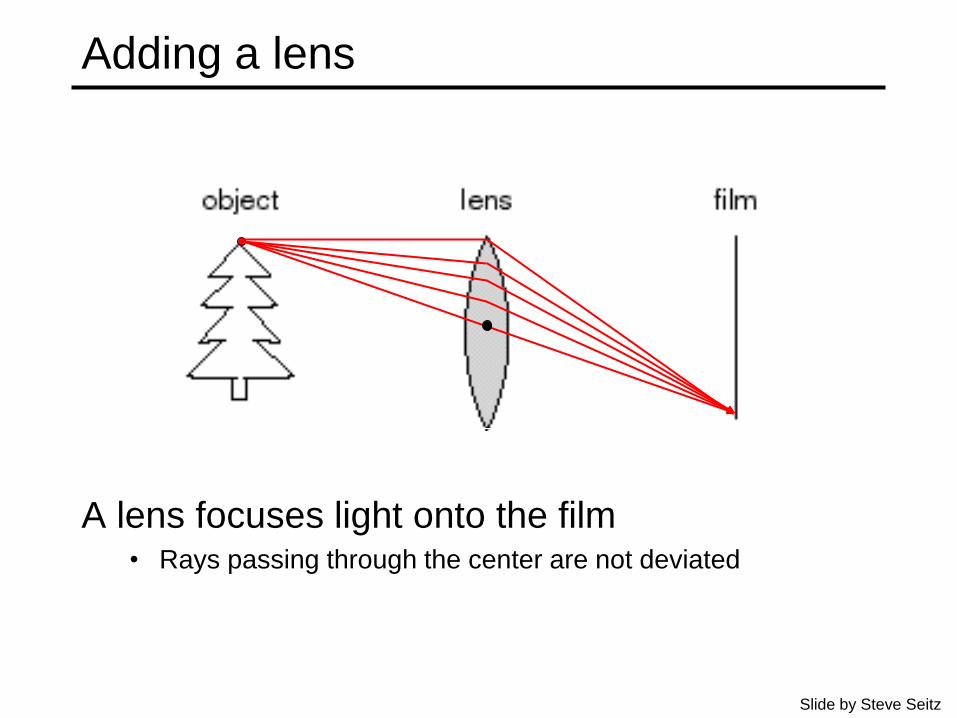
Adding a lens

A lens focuses light onto the film • Rays passing through the center are not deviated

Slide by Steve Seitz

Adding a lens

A lens focuses light onto the film • Rays passing through the center are not deviated

• All parallel rays converge to one point on a plane located at

the focal length f

Slide by Steve Seitz

focal point

f

Adding a lens

A lens focuses light onto the film • There is a specific distance at which objects are ―in focus‖

– other points project to a ―circle of confusion‖ in the image

―circle of

confusion‖

Slide by Steve Seitz

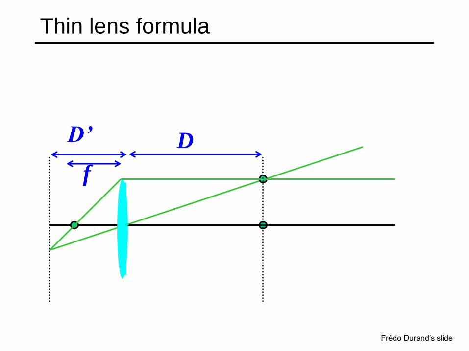
Thin lens formula

f

D D’

Frédo Durand’s slide

Thin lens formula

f

D D’

Similar triangles everywhere!

Frédo Durand’s slide

Thin lens formula

f

D D’

Similar triangles everywhere!

y’

y

y’/y = D’/D

Frédo Durand’s slide

Thin lens formula

f

D D’

Similar triangles everywhere!

y’

y

y’/y = D’/D

y’/y = (D’-f)/f

Frédo Durand’s slide

Thin lens formula

f

D D’

1 D’ D

1 1 f

+ = Any point satisfying the thin lens equation is in focus.

Frédo Durand’s slide

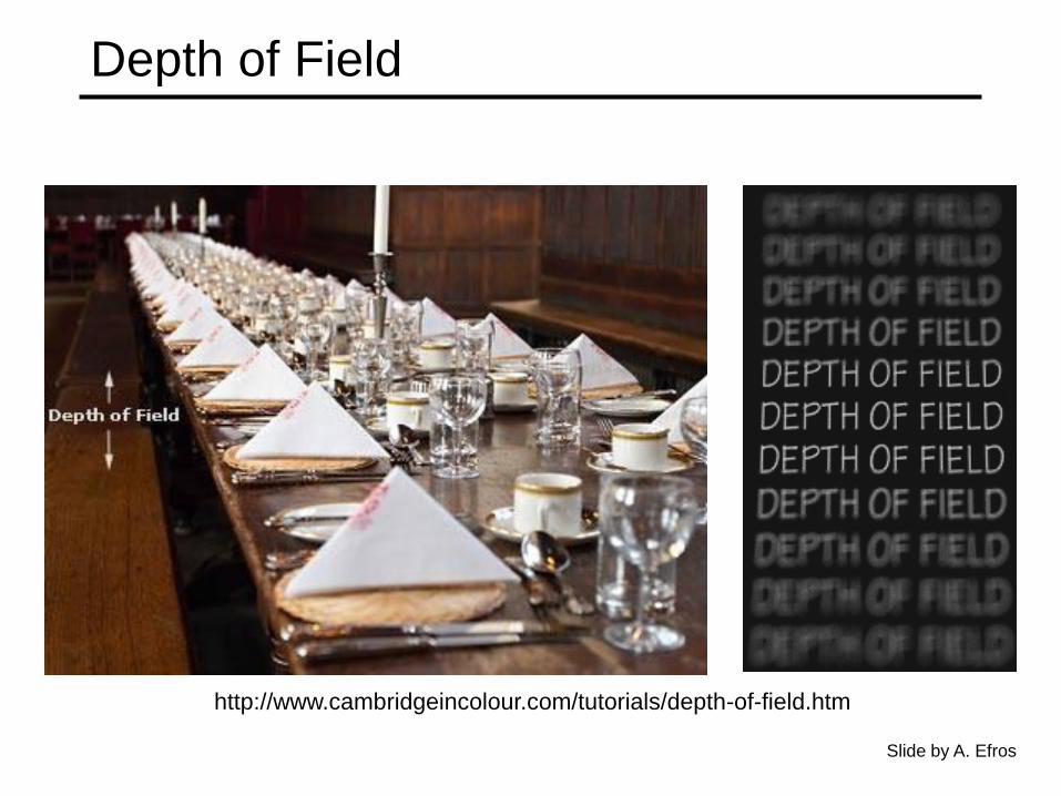
Depth of Field

http://www.cambridgeincolour.com/tutorials/depth-of-field.htm

Slide by A. Efros

Depth of field

Changing the aperture size affects depth of field • A smaller aperture increases the range in which the object is

approximately in focus

f / 5.6

f / 32

Flower images from Wikipedia http://en.wikipedia.org/wiki/Depth_of_field

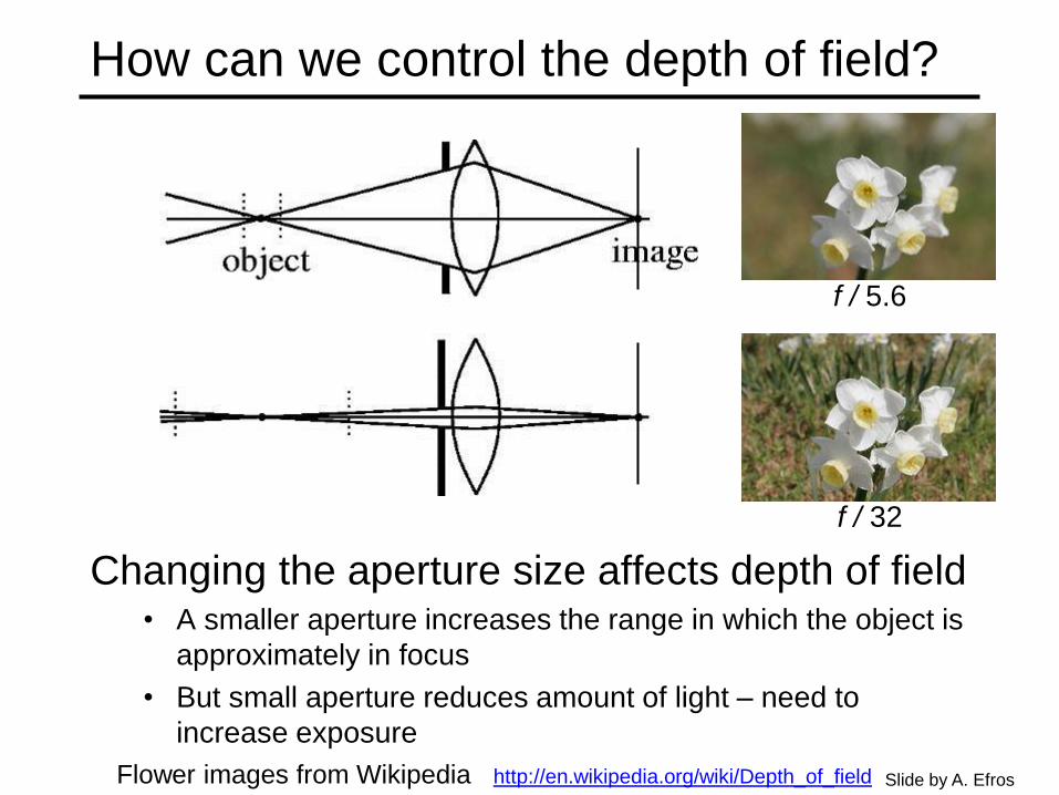
How can we control the depth of field?

Changing the aperture size affects depth of field • A smaller aperture increases the range in which the object is

approximately in focus

• But small aperture reduces amount of light – need to

increase exposure

Slide by A. Efros

f / 5.6

f / 32

Flower images from Wikipedia http://en.wikipedia.org/wiki/Depth_of_field

Varying the aperture

Large aperture = small DOF

Small aperture = large DOF

Slide by A. Efros

Nice Depth of Field effect

Source: F. Durand

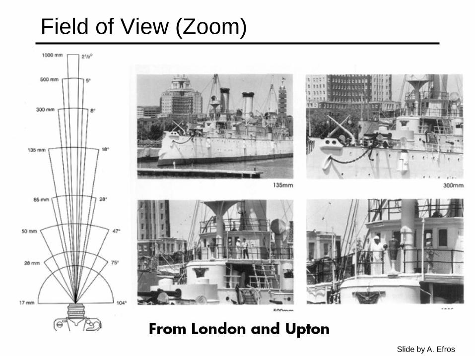
Field of View (Zoom)

Slide by A. Efros

Field of View (Zoom)

Slide by A. Efros

f

Field of View

Smaller FOV = larger Focal Length Slide by A. Efros

f

FOV depends on focal length and size of the camera retina

Field of View / Focal Length

Large FOV, small f

Camera close to car

Small FOV, large f

Camera far from the car

Sources: A. Efros, F. Durand

Same effect for faces

standard wide-angle telephoto

Source: F. Durand

Real lenses

Lens Flaws: Chromatic Aberration

Lens has different refractive indices for different

wavelengths: causes color fringing

Near Lens Center Near Lens Outer Edge

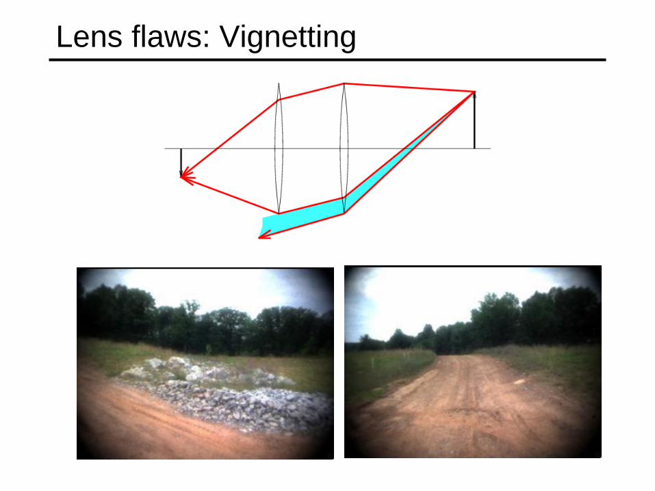
Lens flaws: Vignetting

No distortion Pin cushion Barrel

Radial Distortion

• Caused by imperfect lenses

• Deviations are most noticeable for rays that pass through the edge of

the lens

Distortion

Slides from Seitz

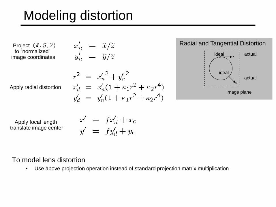
Modeling distortion

To model lens distortion • Use above projection operation instead of standard projection matrix multiplication

Apply radial distortion

Apply focal length translate image center

Project to ―normalized‖

image coordinates

Radial and Tangential Distortion

image plane

ideal actual

ideal actual

Digital camera

A digital camera replaces film with a sensor array • Each cell in the array is light-sensitive diode that converts photons to electrons

• Two common types

– Charge Coupled Device (CCD)

– Complementary metal oxide semiconductor (CMOS)

• http://electronics.howstuffworks.com/digital-camera.htm

Slide by Steve Seitz

CCD vs. CMOS CCD: transports the charge across the chip and reads it at one corner of the array.

An analog-to-digital converter (ADC) then turns each pixel's value into a digital

value by measuring the amount of charge at each photosite and converting that

measurement to binary form

CMOS: uses several transistors at each pixel to amplify and move the charge using

more traditional wires. The CMOS signal is digital, so it needs no ADC.

http://www.dalsa.com/shared/content/pdfs/CCD_vs_CMOS_Litwiller_2005.pdf

http://electronics.howstuffworks.com/digital-camera.htm

High Dynamic Range Images

• CCD / CMOS have a given dynamic range for caputring the luminance of

the scene – LDR cameras (Low Dynamic Range)

• Problem

The dynamic range of the scene illumination is higher than the dynamic of

the camera

• It results

• Saturation areas

• Under exposed areas

High Dynamic Range Images

High dynamic range image - Standard RGB images are encoded over 8 bit integer (255 values)

- HDR: 12 bits floats

+ + + =

See: www.OpenEXR.com

Interlace vs. progressive scan

http://www.axis.com/products/video/camera/progressive_scan.htm Slide by Steve Seitz

Progressive scan

http://www.axis.com/products/video/camera/progressive_scan.htm Slide by Steve Seitz

Interlace

http://www.axis.com/products/video/camera/progressive_scan.htm Slide by Steve Seitz

Color sensing in camera: Color filter array

Source: Steve Seitz

Estimate missing components from neighboring values (demosaicing)

Why more green?

Bayer grid

Human Luminance Sensitivity Function

Color sensing in camera: Prism

• 3 CCD camera • requires three chips and precise alignment

• More expensive

CCD(B)

CCD(G)

CCD(R)

Issues with digital cameras

Noise – low light is where you most notice noise

– light sensitivity (ISO) / noise tradeoff

– stuck pixels

Resolution: Are more megapixels better? – requires higher quality lens

– noise issues

In-camera processing – oversharpening can produce halos

RAW vs. compressed – file size vs. quality tradeoff

Blooming – charge overflowing into neighboring pixels

Color artifacts – purple fringing from microlenses, artifacts from Bayer patterns

– white balance

More info online: • http://electronics.howstuffworks.com/digital-camera.htm

• http://www.dpreview.com/

Slide by Steve Seitz

Historical context

• Pinhole model: Mozi (470-390 BCE),

Aristotle (384-322 BCE)

• Principles of optics (including lenses):

Alhacen (965-1039 CE)

• Camera obscura: Leonardo da Vinci

(1452-1519), Johann Zahn (1631-1707)

• First photo: Joseph Nicephore Niepce (1822)

• Daguerréotypes (1839)

• Photographic film (Eastman, 1889)

• Cinema (Lumière Brothers, 1895)

• Color Photography (Lumière Brothers, 1908)

• Television (Baird, Farnsworth, Zworykin, 1920s)

• First consumer camera with CCD:

Sony Mavica (1981)

• First fully digital camera: Kodak DCS100 (1990)

Niepce, ―La Table Servie,‖ 1822

CCD chip

Alhacen’s notes

Thank You!