3D analysis of pore effect on composite elasticityby means of the finite-element method

Akira Yoneda1 and Ferdous Hasan Sohag1

ABSTRACT

We developed a 3D buffer-layer finite-element method modelto investigate the porosity effect on macroscopic elasticity. Us-ing the 3D model, the effect of pores on bulk effective elasticproperties was systematically analyzed by changing the degreeof porosity, the aspect ratio of the ellipsoidal pore, and the elas-ticity of the material. The results in 3D space were comparedwith the previous results in 2D space. Derivatives of normalizedelastic stiffness constants with respect to needle-type porositywere integers, if the Poisson ratio of a matrix material was zero;those derivatives of normalized stiffness elastic constants forC33, C44, C11, and C66 converged to −1, −2, −3, and −4,

respectively, at the corresponding condition. We have developeda criterion of R < ∼1∕3, where the mutual interaction betweenpores became negligible for macroscopic composite elasticity.These derivatives were nearly constant at less than 5% porosityin the case of a spherical pore, suggesting that the interactionbetween neighboring pores was insignificant if the representa-tive size of the pore was less than one-third of the mean distancebetween neighboring pores. The relations we obtained in thiswork were successfully applied to invert the bulk modulus andrigidity of Cmcm-CaIrO3 as a case study; the performance ofthe inverting scheme was confirmed through this assessment.Thus, our scheme is applicable to predict the macroscopic elas-ticity of porous object as well.

INTRODUCTION

Porous systems are ubiquitous. Sandstone and pumice are porousrocks. Karst terrain is representative of porous structures on theearth (e.g., Hiltunen et al., 2007), and most meteorites and asteroidsalso have significant porosity (Britt et al., 2002). Aside from materi-als associated with earth and planetary sciences, some biological tis-sues, such as those composing trunks and bones, are porous.Furthermore, there are many porous industrial goods, such as rubbersponges, metal foams, and semisintered ceramics. Therefore, themacroscopic physical properties of porous objects have been studiedintensively not only in earth sciences but also in other disciplines,such as material engineering.Composite elasticity of porous objects is of fundamental interest

because of the nontrivial interactions among pores. Although a sin-gle spherical pore in an isotropic elastic body can be analyzedexplicitly by exact analytical solutions, interactions among multiplepores cannot be solved analytically. Therefore, the porosity effect

on composite elasticity has been investigated by various bound meth-ods, such as the Voigt-Reuss bound (Hill, 1952) and the Hashin-Shtrikman bound (Hashin and Shtrikman, 1963). However, it is wellknown that these bounds cannot constrain the composite elasticity ofporous materials in a reasonably narrow range; the lower bounds areinsignificant owing to the infinitely small elasticity of pores (e.g.,Watt, 1976).The differential effective medium (DEM) method, a kind of

self-consistent approach, has been applied to the problem of porousmaterials (e.g., Budiansky, 1965; Hill, 1965; Wu, 1966; Walpole,1969; Guéguen et al., 1997). The validity of the DEM method hasbeen checked using experimental data for specimens of sinteredhard material with porosity. However, it has been difficult to prepareporous specimens with sufficient quality for evaluating the perfor-mance of these theoretical approaches. Thus, the finite-elementmethod (FEM) was introduced to provide unambiguous references(e.g., Berryman, 1995; Mavko et al., 1998; Garboczi and Berry-man, 2001).

Manuscript received by the Editor 29 December 2014; revised manuscript received 14 July 2015; published online 30 November 2015.1Okayama University, Institute for Study of the Earth’s Interior, Tottori, Japan. E-mail: yoneda@misasa.okayama-u.ac.jp; ferdous07@yahoo.com.© The Authors. Published by the Society of Exploration Geophysicists. All article content, except where otherwise noted (including republished material), is

licensed under a Creative Commons Attribution 4.0 Unported License (CC BY). See http://creativecommons.org/licenses/by/4.0/. Distribution or reproduction ofthis work in whole or in part commercially or noncommercially requires full attribution of the original publication, including its digital object identifier (DOI).

L15

GEOPHYSICS, VOL. 81, NO. 1 (JANUARY-FEBRUARY 2016); P. L15–L26, 13 FIGS., 8 TABLES.10.1190/GEO2014-0614.1

We examined the composite elasticity of porous objects by a 3DFEM. An important advantage of the FEM approach is that it candeal with realistic configurations without difficulty; there have beenextensive studies on “digital rock,” i.e., analog models of naturalrock synthesized in a computer by using the FEM and other sim-ulation techniques (e.g., Torquato, 2002; Chen et al., 2007; Nouyand Clement, 2010; Cho et al., 2013). Furthermore, we can extendthe present FEM analysis to anisotropic cases in terms of not onlyphysical properties of the constituent material but also the geometricconfiguration of the pores in 3D space.The present work is a 3D extension of the previous 2D buffered

layer model analysis (Yoneda and Sohag, 2011). The uniqueness ofthe buffered layer model is its regular distribution of pores, which isin distinct contrast to the preceding works based on relativelyirregular geometry (e.g., Cho et al., 2013; Matthies, 2015). Needless

to say, its regularity is definitely more advantageous to evaluate theporosity effect systematically.We have succeeded to obtain various interesting results through

3D FEM analysis. Furthermore, the results were successfully ap-plied to derive intrinsic elasticity of Cmcm-CaIrO3 from its nominalelasticity measured on a porous sample. Cmcm-CaIrO3 is a well-known analog of the postperovskite (PPv) phase in MgSiO3 (Mur-akami et al., 2004; Oganov and Ono, 2004). It is much more elas-tically anisotropic than Pbnm-CaIrO3 of the bridgmanite analog; itcan also be a good analog of crustal anisotropic minerals such asquartz, feldspar, and serpentine (e.g., Vasin et al., 2013; Watanabeet al., 2014).In this work, we limited the present FEM analysis to only a com-

pletely unsaturated dry pore system, although the degree of liquidsaturation in the pores is an important factor for the macroscopicelasticity of porous rock (e.g., Takei, 2002; Vasin et al., 2013).Although it is noted that FEM is inappropriate to simulate nonsta-tionary fluid flow inside pores, the present result is beneficial forexamining porous systems with fluid because it can constrainthe macroscopic elastic property of the porous host rock accommo-dating water or oil.Finally, we follow the Voigt notation for elasticity (stress, σ;

strain, ε; stiffness elastic constant, C; and elastic compliance con-stant, S) throughout this study (e.g., Nye, 1985); it is noted that theVoigt notation is a conventional way to express the exact elasticconstants of a fourth-rank tensor.

PROCEDURES FOR 3D FINITE-ELEMENTMETHOD ANALYSIS

The procedures for 3D FEM analysis are a natural extension ofthose for 2D analysis by Yoneda and Sohag (2011). Because thefundamental concepts and procedures have already been described,we are restricted to a brief description of the procedures of thepresent 3D study.Figure 1 shows an octant part of the 5 × 5 × 5 buffered layer

model used in the present 3D analysis; the figures in Appendix Bshow some extreme cases with mesh density. Although the outer-most edge length is set as 1 m in the present work for simplicity, theabsolute size of the geometry does not matter for the present pur-pose. This means that the ratio between the edge length and thediameter of the pore is essential. Considering the symmetry alongthe central interfaces, FEM analysis can be conducted only on anoctant part. In this work, we conducted FEM analysis using COM-SOL®, which is commercial FEM software.Figure 2 shows the ellipsoidal shape of pores discussed in this

study. The three principal axes of the ellipsoid were set as a, b,and c in the x-, y-, and z-directions, respectively. To decrease thecomplexity, we assume a ¼ b, and we adjust að¼ bÞ and c. Here,the inverse of the aspect ratio α 0ð¼ a∕cÞ is introduced to describethe present results; note that the definition of α 0 is inverse of theaspect ratio that is usually used in poroelasticity.Here, we summarize the essence of the present model geometries:

(1) Pores are embedded in an elastically isotropic matrix. (2) Poresare all identical, and (3) their centers distribute regularly at gridpoints in a model geometry. (4) Symmetric axes of pores align al-ways in the z-axis direction.Because of the equivalence between the x- and y-directions, the

porous bodies analyzed in this study have tetragonal symmetry. Inthe spherical pores cases, it has cubic symmetry because of the

Figure 1. Octant part of a multi-buffer-layer model for N ¼ 5, ora 5 × 5 × 5 model with a cube having an edge length of 1 m. Theedges of the central cube, indicated by short arrows, correspond tothe observation interfaces for stress and displacement in the defor-mation tests.

Figure 2. Examples of the shape of a pore as a function of aspectratio α 0. In this drawing, the size of the pores is normalized to havethe same volume.

L16 Yoneda and Sohag

regular distribution of pores. The terminologies of “tetragonal” and“cubic” symmetry for investigated bodies are based on an analogyof those symmetries defined in crystallography.After setting the model geometry as described above, uniform

displacements were applied to the outer surfaces of the model ge-ometry to generate a stress-strain relation inside the model. In thiswork, the matrix was first assumed to be elastically isotropic with aYoung modulus Y ¼ 100 GPa; the Poisson ratio ν was treated as avariable between 0 and 0.45.Let us define u, v, and w as displacements in the x-, y-, and z-

directions, respectively. In the 3D analysis, we can classify six typesof forced displacement on the outermost surfaces as follows:(1) There is uniform forced displacement of Δu ¼ −1 × 10−6 m

in the x-direction on the x-surface, whereas the model is free in they- and z-directions, or there is no constraint on the y- and z-surfaces.Cases (2) and (3) are similar to (1), but the directions of compres-sion are in the y- and z-directions, respectively. (4) There is acoupled uniform forced displacement of Δv ¼ 1 × 10−6 m in they-direction on the z-surface, and that of Δw ¼ 1 × 10−6 in thez-direction on the y-surface. This is a pure shear deformation ob-served from the x-direction. Cases (5) and (6) are similar to (4), butcorresponding pure shear deformations are observed from they- and z-directions, respectively.We easily obtain the average strains from the resulting displace-

ments Δu, Δv, and Δw along the observation interfaces:

ε1¼Δux0

; ε2¼Δvy0

; ε3¼Δwz0

;

ε4¼�Δvz0

þΔwy0

�; ε5¼

�Δwz0

þΔux0

�; and ε6¼

�Δuy0

þΔvx0

�;

(1)

where the overbar for Δu, Δv, and Δw specifies their average, andx0, y0, and z0 are the positions of the observation interfaces in the x-,y-, and z-coordinates, respectively. We then formulate the simulta-neous equations between the averaged stresses over the observedinterface and those averaged strains:

σ1 ¼ C11ε1 þ C12ε2 þ C13ε3;

σ2 ¼ C12ε1 þ C11ε2 þ C13ε3;

σ3 ¼ C13ε1 þ C13ε2 þ C33ε3. (2)

We can make three sets of simultaneous equations according tothe uniaxial compressions in the x-, y-, and z-directions. In general,we have nine redundant equations for four unknown parameters,C11ð¼ C22Þ, C12, C13ð¼ C23Þ, and C33. These four parameters weresolved using the least-squares method. For two independent shearelastic constants C44ð¼ C55Þ and C66, we have the following equa-tions:

σ4 ¼ C44ε4; σ6 ¼ C66ε6. (3)

Here, we introduce normalized moduli C�ð¼ C∕C0Þ, where C0 isthe modulus of the matrix material itself or that of the porous systemat zero porosity. According to the experience of the previous 2D

analysis (Yoneda and Sohag, 2011), we would mainly observethe initial slope of the normalized elastic constant against porosityϕ, defined as

Dijðα 0; νÞ ¼ limϕ→0

∂C�ijðϕ; α 0; νÞ∂ϕ

: (4)

The usefulness of C� and D were well confirmed in the previous2D analysis (Yoneda and Sohag, 2011).

RESULTS AND DISCUSSION

We start with the case of a spherical pore in a matrix with a Pois-son ratio of ν ¼ 0.3 as the simplest representative case. Figure 3shows the variations in the longitudinal and shear elastic constants(CP and CS) as functions of porosity obtained using the FEM andDEM methods, respectively. Although the DEM calculation wasconducted to 100% porosity, the FEM calculation was terminatedat 50% porosity to avoid mutual contact between neighboring poresat 0.5236, which is the volume ratio between a cube and its inscribedsphere. We recognize that the porous object still has substantialstiffness to the limit of contact between neighboring spherical pores.This contrasts with the 2D analysis, in which the object loses stiffnesswhen approaching the limit of circular pore contact. This is anobvious dimensional effect between the 2D and 3D analyses.In the case of a spherical pore, the macroscopic object maintains

cubic symmetry, where C11 ¼ C22 ¼ C33, C12 ¼ C23 ¼ C31, andC44 ¼ C55 ¼ C66 are satisfied. The general trend of the FEM resultsis similar to that estimated by the DEM method. The DEM resultsare consistent with the most compliant elastic constant in the presentFEM analysis. This is consistent with the preliminary results ob-tained in the 2D analysis (Figure 14 in Yoneda and Sohag, 2011).Figure 3 also shows that the directional fluctuations of CP and CS

are approximately 20% and 33%, respectively, at approximately50% porosity. The directional anisotropy is smaller than those in2D analysis, where we recognized more than 25% and 75% direc-tional fluctuation, respectively, at approximately 50% porosity(Figure 5 in Yoneda and Sohag, 2011).Further, we recognize that the macroscopic elasticity of the

porous object is nearly isotropic and has a linear change in thelow-porosity range (< 5%) for the longitudinal and shear stiffnessconstants. This observation is analogous to the case in 2D analysis.This finding suggests an important concept that the pore effectcan be treated as a “linear system” in the porosity range lower thanapproximately 5%. In other words, we expect “additivity” amongpores with different shapes, sizes, and orientations as long as thedistribution of pores is homogeneous and the porosity is lowenough. Let us define the ratio R ¼ l∕d (l, a representative size ofa pore, and d, the distance between the nearest pores); R is intro-duced as a scale for evaluating mutual interaction among pores. Weconclude that for R < ∼1∕3 (approximately 0.37, or the cubic rootof 0.05), where the mutual interaction between pores is negligiblefor macroscopic composite elasticity. If the shape and distributionof pores are anisotropic and/or heterogeneous, we should use amaximum l and a minimum d when evaluating R.Figure 4 compares D values derived using the FEM and DEM

methods in the spherical pore case. We can see that the presentFEM results are consistent with those of the DEM method, assuggested in previous works (e.g., Matthies, 2015).

3D pore effect on composite elasticity L17

We recognize that the 5 × 5 × 5 model shows better consistencywith DEM results than does the 7 × 7 × 7 model. This situation iscaused by the limitation of machine capacity making a precise meshin the 7 × 7 × 7 model. Therefore, we use the 5 × 5 × 5 modelbecause of the better consistency with the DEM method in thiswork.

According to an analogy with the previous 2D analysis, we firstcheck the relation between theD values and aspect ratio α 0 at ν ¼ 0.We find the following from Figure 5:

1) D33 converges to −1 as α 0 → 0. This is consistent with intuitionbecause the pores approach tubes extending in the z-direction atthe limit of α 0 → 0.

2) D11 and D66 converge to −3 and −4, respectively, as α 0 → 0.This is consistent with the previous 2D analysis because of thegeometric similarity.

Figure 3. Decrease in elastic constants with porosity ϕ in a repre-sentative case of a spherical pore (α 0 ¼ 1.0) and ν ¼ 0.3. FEM re-sults (solid lines) and DEM results (dashed line) are compared. Notethat the present FEM analysis is limited at approximately 50%because of the contact between neighboring spheres. (a) CP elasticstiffness constants corresponding to longitudinal waves. For FEMresults, the symbols “○,” “□,” and “△” are used to specify thecurves of C11, ðC11 þ C12 þ 2C44Þ∕2, and ðC11 þ 2C12 þ 4C44Þ∕3, corresponding to longitudinal waves in the [100], [110], and[111] directions, respectively. (b) CS elastic stiffness constants cor-responding to S-waves. For FEM results, the symbols “○,” “□,”and “△” are used to specify curves of C44, ðC11 − C12Þ∕2, andðC11 − C12 þ C44Þ∕3, corresponding S-waves in the [100], [110],and [111] directions, respectively.

Figure 4. The D11 ð¼ D22; D33Þ and D44 ð¼ D55; D66Þ versus thePoisson ratio ν for a spherical pore, or aspect ratio α 0 ¼ 1. Thedashed lines are the results obtained using the DEM method. Sym-bols “○” and “▪” are used to show the results of the 5 × 5 × 5 and7 × 7 × 7 FEM models, respectively. Note that the result obtainedusing the 7 × 7 × 7 model at ν ¼ 0.45 is not shown because of di-vergence in the FEM calculation.

Figure 5. The D11 ð¼ D22Þ, D33, D44 ð¼ D55Þ, and D66 versus as-pect ratio α 0 between 0.1 and 10 at a Poisson ratio ν ¼ 0.

L18 Yoneda and Sohag

3) D44 converges to −2 as α 0 → 0. This is a new finding of thepresent 3D analysis. Consequently,D33,D44,D11, andD66 con-verge to −1, −2, −3, and −4, respectively, at ν ¼ 0 andas α 0 → 0.

4) D11 and D66 converge to −1 as α 0 → ∞, whereas D33 and D44

diverge to −∞ as α 0 → ∞. This is consistent with intuition be-cause the pores approach plates in the x − y space at the limitof α 0 → ∞.

5) At α 0 ¼ 1, all theDij values are close to −2, which is consistentwith previous analysis for selected moduli by means of the self-consistent method, DEM, etc. (e.g., Guéguen et al., 1997; Choet al., 2013; Matthies, 2015).

Although our findings (equations 2 and 3) are difficult not only tounderstand intuitively but also to derive deductively, they are inter-

esting and useful to qualitatively predict the macroscopic elasticityof porous object.In the previous 2D analysis of a circular pore, we found useful

relations consistent with 2D FEM results, such as those for a cir-cular pore:

D11ðνÞ ¼ −3þ 8νð0.25 − νÞð1 − 2νÞ ; D66ðνÞ ¼ −4ð1 − νÞ: (5)

We tried to find similar relations for 3D FEM analysis, startingwith the analogous functional forms used in 2D analysis. We as-sumed the following functional forms for longitudinal and shearconstants:

Figure 6. Performance of the fitting functions of equations 6 and 7 (solid line) against the FEM results (“*”) in the Poisson ratio range ofν ¼ 0.0 − 0.4. The three cases of α 0 ¼ 0.1, 1.0, and 10.0 correspond to plots (a-c), respectively.

3D pore effect on composite elasticity L19

D11ðα 0; νÞ ¼ −p1ðα 0Þ þ p2ðα 0Þνðp3ðα 0Þ − νÞð1 − 2νÞ ;

D33ðα 0; νÞ ¼ −q1ðα 0Þ þ q2ðα 0Þνðq3ðα 0Þ − νÞð1 − 2νÞ ; (6)

D44ðα 0; νÞ ¼ −r1ðα 0Þð1 − r2ðα 0ÞνÞr3ðα 0Þ;

D66ðα 0; νÞ ¼ −s1ðα 0Þð1 − s2ðα 0ÞνÞs3ðα 0Þ: (7)

Figure 6 shows the results of fitting equations 6 and 7 to the FEMresults. We recognize that the functions reproduced the FEM resultsreasonably. The differences between the FEM results and the fittingvalues are within approximately 1.0 for D11 and D33, and approx-imately 0.1 for D44 and D66, for the fitting range of ν from 0.0 to0.4. It is worth mentioning that the fitting performance improves toapproximately 0.2 for D11 and D33, and approximately 0.1 for D44

and D66, for the fitting range of ν from 0.0 to 0.35. Figure 7 showsthe resulting variations in the parameters p, q, r, and s with aspectratio α 0 for the fitting range of ν from 0.0 to 0.4. It is worth men-tioning that the global features of p, q, r, and s are similar for thefitting range of ν from 0.0 to 0.35 as well.Finally, the fittings for D12 and D23 are mentioned. According to

analogy with the previous 2D analysis, we tested the followingfunctional forms to find a suitable functional form inductively:

D12ðα 0; νÞ ¼ 1

C012

fC011D11 þ 2C0

66D66Þg; (8)

D23ðα 0; νÞ ¼ 1

C012

�C011ðD11 þD33Þ

2þ C0

66ðD44 þD66Þ�.

(9)

Figure 8 compares the results of fitting equations 8 and 9 to theFEM results. We see that the performance of the functions is notsatisfactory except for α 0 ¼ 1.0 and ν of 0.1–0.3. This is in contrastwith the previous 2D study, where an equation analogous withequations 8 and 9 worked very well (see equation 20 and Figure 10in Yoneda and Sohag, 2011). The survey for more suitable fictionalforms in 3D remains as a future subject.The data sets of the D values are given in Appendix A, and we

recommend that readers carry out their own fitting of the dataaround specific values of ν and α 0 using equations 6–9, a splinefunction, polynomial function, or another function.

CASE STUDY ON POROUS Cmcm-CaIrO3

AGGREGATE

Cmcm-CaIrO3 has been frequently investigated as a representa-tive analog of unquenchable PPv-MgSiO3 (e.g., Hunt et al. 2009),since Murakami et al. (2004) and Oganov and Ono (2004) discoverthe PPv phase in MgSiO3 with Cmcm-CaIrO3 structure. Yonedaet al. (2014) report single crystal elasticity of Cmcm-CaIrO3 bymeans of the inelastic X ray scattering (IXS) technique (Table 1).Before the single crystal elasticity of Cmcm-CaIrO3 was avail-

able, ultrasonic velocity was measured on a porous aggregate ofCmcm-CaIrO3 synthesized at 8 GPa and 1200°C in the Kawai-typehigh-pressure apparatus. The specimen was confirmed to be a singlephase of Cmcm-CaIrO3 by means of X-ray diffraction. Figure 9 is asectional image of the specimen showing the pore shape (α 0 ∼ 0.3)and distribution; its porosity was estimated to be 6% by comparingits nominal density and the X-ray density of 8211 kg∕m3 (Sugaharaet al., 2008).We measured ultrasonic velocities in the three directions of a

rectangular specimen (approximately 1 mm edge length), and wefound it to be nearly isotropic within 2% in P-and S-wave velocities.

Figure 7. Resulting parameters p, q, r, and s as functions of aspectratio α 0, after the fitting of the FEM results based on equations 6 and7 (see Figure 6). The solid, dashed, and dotted lines correspond tosubscripts of 1, 2, and 3 for p, q, r, and s, respectively. A significantanomaly for r2 (the dashed curve in the D44 plot) at the left end ofthe plot area seems to be due to numerical instability.

Figure 8. D12 versus the Poisson ratio ν at aspect ratio α 0 ¼ 0.1,1.0, and 10. The solid lines are calculated using equation 8, andthe dashed lines are calculated using equation 9, and the symbols“●” and “○” show the D12 and D23 obtained in FEM analysis.

L20 Yoneda and Sohag

Liu et al. (2011) do independent study on Cmcm-CaIrO3 aggregatessynthesized by themselves (8% porosity); those results are summa-rized in Table 2 with nominal values of bulk modulus and rigidity; thetwo experimental data agree well with each other despite the 2%porosity difference.The experimental data are enough to constrain intrinsic K and G

from the four parameters of the porous object (porosity, aspect ratioof pore, and P- and S-wave velocities) as suggested in previous re-search (e.g., Takei, 2002). Thus, we tried to correct the nominalvalues of the bulk modulus and rigidity to the intrinsic ones by usingthe results of the present FEM analysis.The present target specimen was assumed to be a macroscopi-

cally isotropic elastic object, whereas the present FEM porosity ef-fect analysis was conducted on an object with tetragonal symmetry(equivalence between the x- and y-directions) resulting inD11 ¼ D22,D13 ¼ D23, andD44 ¼ D55. We have to take that differ-ence into account in conducting the porosity effect correction.The correction of the porosity effect was conducted using the

following method: The initial values for Cð0Þ11 ð¼ Cð0Þ

22 ; Cð0Þ33 Þ,

Cð0Þ12 ð¼ Cð0Þ

23 ; Cð0Þ31 Þ, and Cð0Þ

44 ð¼ Cð0Þ55 ; C

ð0Þ66 Þ were calculated to be

251, 101, and 75 GPa from the present 6% porosity object; thesuperscript suffix “0” indicates the initial value of the iterative proc-ess. It is noted that C11, C12, and C44 are equivalent with λþ 2μ, λ,and μð¼ GÞ, respectively, by using Lame’s elastic constants for iso-tropic elasticity.The porosity effect was corrected according to

Cðiþ1Þ11 ¼ Cð0Þ

11 f1 − 0.02 × ½D11ðα; νðiÞÞþD22ðα; νðiÞÞ þD33ðα; νðiÞÞ�g;

Cðiþ1Þ12 ¼ Cð0Þ

12 f1 − 0.02 × ½D12ðα; νðiÞÞþD23ðα; νðiÞÞ þD31ðα; νðiÞÞ�g;

Cðiþ1Þ44 ¼ Cð0Þ

44 f1 − 0.02 × ½D44ðα; νðiÞÞþD55ðα; νðiÞÞ þD66ðα; νðiÞÞ�g;

(10)

where α 0 was fixed at approximately 0.3, and νðiÞ

was recalculated each time from CðiÞ11 , C

ðiÞ12 , and

CðiÞ44 , at the ith iteration. The factor of “0.02”

in equation 10 is one-third of the 6% porosity,which was equally divided into the three direc-tions of the x-, y-, and z-axes. In the present iter-ation, νðiÞ was slightly shifted from 0.285 to0.287 throughout.

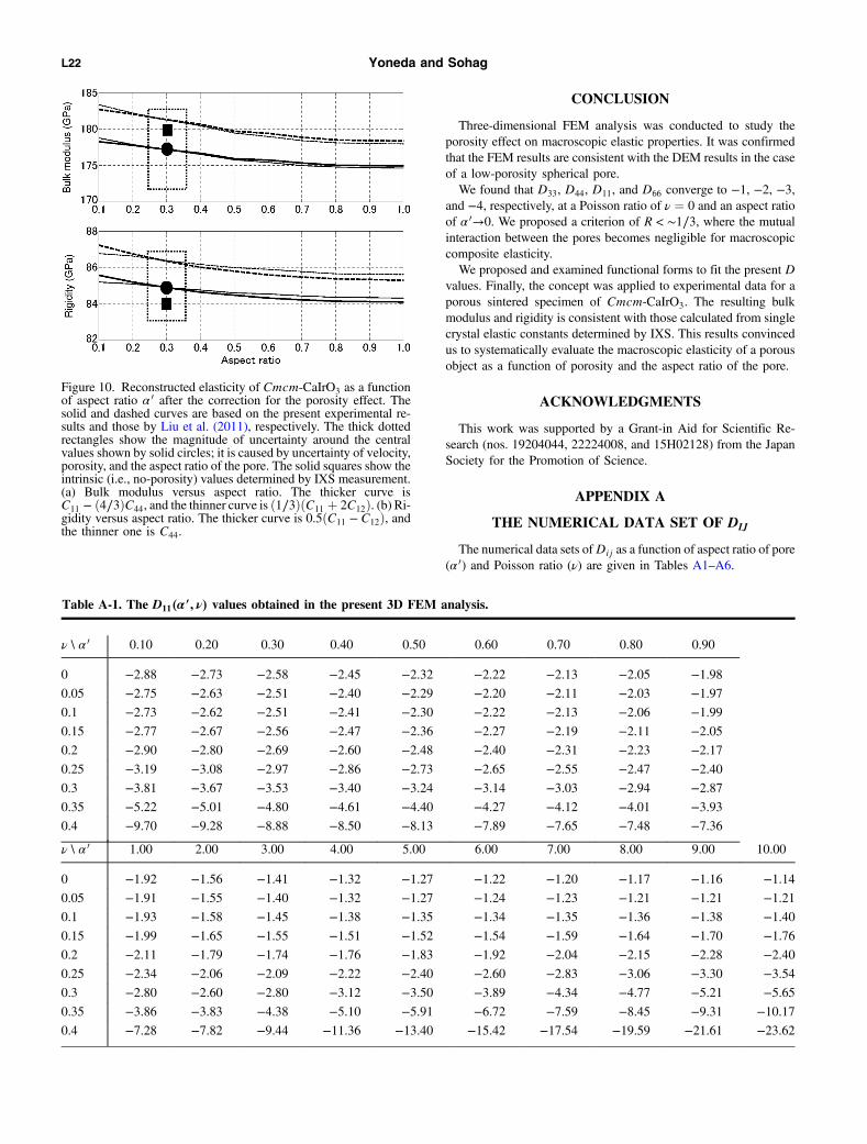
Figure 10 shows the results of the correction for the porosityeffect. We found that K ¼ 177ð6Þ GPa and G ¼ 85ð2Þ GPa, wherethe magnitude of error was estimated from the uncertainty inaspect ratio α 0, porosity, and the anisotropy of the ultrasonic veloc-ities. We recognize that the present results are consistent with theintrinsic bulk modulus and rigidity (178 and 84 GPa as shownin Table 1) within the uncertainties. Thus, the present case studyconfirms the reliability of the present correction procedure forthe porosity effect.

Figure 9. Scanning electron microscope image of the Cmcm-CaIrO3 specimen with 6% porosity. The black parts correspond topores, suggesting a tubelike geometry. Although it is difficult todetermine the average aspect ratio α 0 of pores from the image,we used α 0 ∼ 0.3 as the starting value of the correction for theporosity effect.

Table 1. Single-crystal elastic constants of Cmcm-CaIrO3 (upper row) and Pbnm-CaIrO3 (lower row) determined by IXS(Yoneda et al., 2014). The unit is in gigapascal. Uncertainties are shown in parentheses. The values KH and GH are the Voigt-Reuss-Hill average of the bulk modulus and rigidity, respectively.

C11 C22 C33 C12 C23 C31 C44 C55 C66 KH GH

378 (4) 255 (11) 360 (5) 104 (7) 137 (9) 73 (6) 76 (5) 56 (2) 85 (3) 178 (4) 84 (1)

235 (6) 278 (6) 286 (11) 132 (6) 138 (11) 120 (10) 87 (4) 60 (2) 79 (2) 174 (6) 72 (2)

Table 2. Results of velocity measurement on the porous Cmcm-CaIrO3 aggre-gate. In the present study, the P- and S-wave velocities were measured by 50-and 20-MHz transducers, respectively. Uncertainties are shown in parentheses.Elastic moduli were calculated assuming isotropic elasticity; λ is one of Lame’selastic constants corresponding to C12.

Data source Porosity VP (km∕s) VS (km∕s) K (GPa) G (GPa) λ (GPa)

Liu et al. (2011) 8% 5.71 (3) 3.13 (2) 148 74 99

Present study 6% 5.7 (1) 3.13 (2) 151 (5) 75 (1) 101

3D pore effect on composite elasticity L21

CONCLUSION

Three-dimensional FEM analysis was conducted to study theporosity effect on macroscopic elastic properties. It was confirmedthat the FEM results are consistent with the DEM results in the caseof a low-porosity spherical pore.We found that D33, D44, D11, and D66 converge to −1, −2, −3,

and −4, respectively, at a Poisson ratio of ν ¼ 0 and an aspect ratioof α 0→0. We proposed a criterion of R < ∼1∕3, where the mutualinteraction between the pores becomes negligible for macroscopiccomposite elasticity.We proposed and examined functional forms to fit the present D

values. Finally, the concept was applied to experimental data for aporous sintered specimen of Cmcm-CaIrO3. The resulting bulkmodulus and rigidity is consistent with those calculated from singlecrystal elastic constants determined by IXS. This results convincedus to systematically evaluate the macroscopic elasticity of a porousobject as a function of porosity and the aspect ratio of the pore.

ACKNOWLEDGMENTS

This work was supported by a Grant-in Aid for Scientific Re-search (nos. 19204044, 22224008, and 15H02128) from the JapanSociety for the Promotion of Science.

APPENDIX A

THE NUMERICAL DATA SET OF DIJ

The numerical data sets ofDij as a function of aspect ratio of pore(α 0) and Poisson ratio (ν) are given in Tables A1–A6.

Figure 10. Reconstructed elasticity of Cmcm-CaIrO3 as a functionof aspect ratio α 0 after the correction for the porosity effect. Thesolid and dashed curves are based on the present experimental re-sults and those by Liu et al. (2011), respectively. The thick dottedrectangles show the magnitude of uncertainty around the centralvalues shown by solid circles; it is caused by uncertainty of velocity,porosity, and the aspect ratio of the pore. The solid squares show theintrinsic (i.e., no-porosity) values determined by IXS measurement.(a) Bulk modulus versus aspect ratio. The thicker curve isC11 − ð4∕3ÞC44, and the thinner curve is ð1∕3ÞðC11 þ 2C12Þ. (b) Ri-gidity versus aspect ratio. The thicker curve is 0.5ðC11 − C12Þ, andthe thinner one is C44.

Table A-1. The D11�α 0; ν� values obtained in the present 3D FEM analysis.

ν \ α 0 0.10 0.20 0.30 0.40 0.50 0.60 0.70 0.80 0.90

0 −2.88 −2.73 −2.58 −2.45 −2.32 −2.22 −2.13 −2.05 −1.980.05 −2.75 −2.63 −2.51 −2.40 −2.29 −2.20 −2.11 −2.03 −1.970.1 −2.73 −2.62 −2.51 −2.41 −2.30 −2.22 −2.13 −2.06 −1.990.15 −2.77 −2.67 −2.56 −2.47 −2.36 −2.27 −2.19 −2.11 −2.050.2 −2.90 −2.80 −2.69 −2.60 −2.48 −2.40 −2.31 −2.23 −2.170.25 −3.19 −3.08 −2.97 −2.86 −2.73 −2.65 −2.55 −2.47 −2.400.3 −3.81 −3.67 −3.53 −3.40 −3.24 −3.14 −3.03 −2.94 −2.870.35 −5.22 −5.01 −4.80 −4.61 −4.40 −4.27 −4.12 −4.01 −3.930.4 −9.70 −9.28 −8.88 −8.50 −8.13 −7.89 −7.65 −7.48 −7.36

ν \ α 0 1.00 2.00 3.00 4.00 5.00 6.00 7.00 8.00 9.00 10.00

0 −1.92 −1.56 −1.41 −1.32 −1.27 −1.22 −1.20 −1.17 −1.16 −1.140.05 −1.91 −1.55 −1.40 −1.32 −1.27 −1.24 −1.23 −1.21 −1.21 −1.210.1 −1.93 −1.58 −1.45 −1.38 −1.35 −1.34 −1.35 −1.36 −1.38 −1.400.15 −1.99 −1.65 −1.55 −1.51 −1.52 −1.54 −1.59 −1.64 −1.70 −1.760.2 −2.11 −1.79 −1.74 −1.76 −1.83 −1.92 −2.04 −2.15 −2.28 −2.400.25 −2.34 −2.06 −2.09 −2.22 −2.40 −2.60 −2.83 −3.06 −3.30 −3.540.3 −2.80 −2.60 −2.80 −3.12 −3.50 −3.89 −4.34 −4.77 −5.21 −5.650.35 −3.86 −3.83 −4.38 −5.10 −5.91 −6.72 −7.59 −8.45 −9.31 −10.170.4 −7.28 −7.82 −9.44 −11.36 −13.40 −15.42 −17.54 −19.59 −21.61 −23.62

L22 Yoneda and Sohag

Table A-2. The D33�α 0; ν� values obtained in the present 3D FEM analysis.

ν \ α 0 0.10 0.20 0.30 0.40 0.50 0.60 0.70 0.80 0.90

0 −1.05 −1.12 −1.20 −1.28 −1.38 −1.48 −1.59 −1.69 −1.810.05 −1.08 −1.15 −1.21 −1.29 −1.38 −1.49 −1.59 −1.69 −1.800.1 −1.14 −1.20 −1.26 −1.33 −1.42 −1.52 −1.62 −1.71 −1.820.15 −1.23 −1.28 −1.34 −1.41 −1.49 −1.58 −1.68 −1.77 −1.880.2 −1.39 −1.44 −1.48 −1.54 −1.61 −1.71 −1.80 −1.89 −2.000.25 −1.69 −1.72 −1.75 −1.80 −1.86 −1.95 −2.03 −2.12 −2.230.3 −2.27 −2.27 −2.28 −2.31 −2.35 −2.43 −2.50 −2.59 −2.690.35 −3.61 −3.55 −3.50 −3.48 −3.47 −3.53 −3.58 −3.65 −3.750.4 −8.00 −7.73 −7.50 −7.32 −7.16 −7.12 −7.08 −7.10 −7.18

ν \ α 0 1.00 2.00 3.00 4.00 5.00 6.00 7.00 8.00 9.00 10.00

0 −1.92 −3.11 −4.33 −5.55 −6.78 −7.97 −9.18 −10.39 −11.56 −12.760.05 −1.91 −3.10 −4.32 −5.56 −6.80 −8.00 −9.23 −10.45 −11.63 −12.850.1 −1.93 −3.13 −4.37 −5.62 −6.89 −8.11 −9.36 −10.60 −11.80 −13.040.15 −1.99 −3.20 −4.47 −5.76 −7.06 −8.32 −9.61 −10.89 −12.13 −13.410.2 −2.11 −3.35 −4.68 −6.03 −7.39 −8.71 −10.07 −11.41 −12.71 −14.050.25 −2.34 −3.64 −5.06 −6.51 −7.98 −9.41 −10.88 −12.32 −13.73 −15.170.3 −2.80 −4.20 −5.79 −7.43 −9.10 −10.72 −12.38 −14.03 −15.62 −17.250.35 −3.86 −5.46 −7.41 −9.44 −11.52 −13.53 −15.61 −17.64 −19.63 −21.640.4 −7.28 −9.46 −12.47 −15.66 −18.93 −22.09 −25.34 −28.49 −31.55 −34.62

Table A-3. The D44�α 0; ν� values obtained in the present 3D FEM analysis.

ν \ α 0 0.10 0.20 0.30 0.40 0.50 0.60 0.70 0.80 0.90

0 −1.99 −1.96 −1.95 −1.95 −1.97 −1.99 −2.02 −2.05 −2.090.05 −1.99 −1.95 −1.93 −1.92 −1.93 −1.95 −1.97 −2.00 −2.030.1 −1.98 −1.94 −1.91 −1.90 −1.91 −1.92 −1.94 −1.96 −2.000.15 −1.98 −1.93 −1.90 −1.88 −1.89 −1.89 −1.91 −1.93 −1.960.2 −1.98 −1.91 −1.88 −1.86 −1.86 −1.86 −1.88 −1.89 −1.920.25 −1.97 −1.90 −1.86 −1.83 −1.83 −1.83 −1.84 −1.85 −1.870.3 −1.97 −1.89 −1.84 −1.81 −1.80 −1.79 −1.80 −1.81 −1.830.35 −1.96 −1.87 −1.81 −1.77 −1.76 −1.75 −1.75 −1.76 −1.770.4 −1.95 −1.85 −1.78 −1.74 −1.72 −1.70 −1.70 −1.70 −1.71

ν \ α 0 1.00 2.00 3.00 4.00 5.00 6.00 7.00 8.00 9.00 10.00

0 −2.13 −2.65 −3.24 −3.84 −4.46 −5.08 −5.70 −6.32 −6.94 −7.560.05 −2.07 −2.55 −3.10 −3.67 −4.26 −4.84 −5.43 −6.01 −6.61 −7.190.1 −2.03 −2.49 −3.02 −3.58 −4.14 −4.71 −5.28 −5.85 −6.42 −7.000.15 −1.99 −2.43 −2.94 −3.48 −4.02 −4.57 −5.13 −5.68 −6.23 −6.780.2 −1.95 −2.36 −2.85 −3.37 −3.90 −4.42 −4.96 −5.49 −6.03 −6.560.25 −1.90 −2.29 −2.76 −3.25 −3.76 −4.27 −4.78 −5.29 −5.81 −6.320.3 −1.85 −2.21 −2.66 −3.13 −3.62 −4.10 −4.59 −5.08 −5.58 −6.060.35 −1.79 −2.13 −2.55 −3.00 −3.46 −3.92 −4.39 −4.85 −5.33 −5.790.4 −1.72 −2.04 −2.43 −2.86 −3.29 −3.73 −4.17 −4.61 −5.06 −5.49

3D pore effect on composite elasticity L23

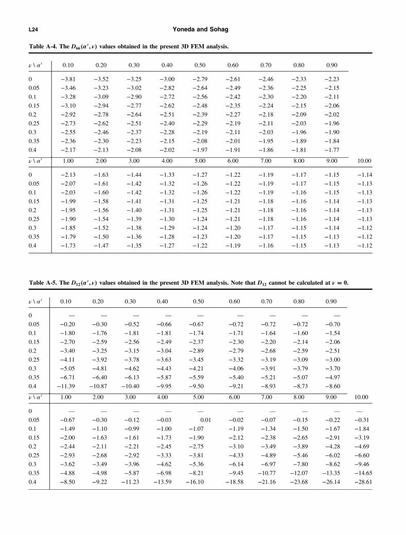
Table A-4. The D66�α 0; ν� values obtained in the present 3D FEM analysis.

ν \ α 0 0.10 0.20 0.30 0.40 0.50 0.60 0.70 0.80 0.90

0 −3.81 −3.52 −3.25 −3.00 −2.79 −2.61 −2.46 −2.33 −2.230.05 −3.46 −3.23 −3.02 −2.82 −2.64 −2.49 −2.36 −2.25 −2.150.1 −3.28 −3.09 −2.90 −2.72 −2.56 −2.42 −2.30 −2.20 −2.110.15 −3.10 −2.94 −2.77 −2.62 −2.48 −2.35 −2.24 −2.15 −2.060.2 −2.92 −2.78 −2.64 −2.51 −2.39 −2.27 −2.18 −2.09 −2.020.25 −2.73 −2.62 −2.51 −2.40 −2.29 −2.19 −2.11 −2.03 −1.960.3 −2.55 −2.46 −2.37 −2.28 −2.19 −2.11 −2.03 −1.96 −1.900.35 −2.36 −2.30 −2.23 −2.15 −2.08 −2.01 −1.95 −1.89 −1.840.4 −2.17 −2.13 −2.08 −2.02 −1.97 −1.91 −1.86 −1.81 −1.77

ν \ α 0 1.00 2.00 3.00 4.00 5.00 6.00 7.00 8.00 9.00 10.00

0 −2.13 −1.63 −1.44 −1.33 −1.27 −1.22 −1.19 −1.17 −1.15 −1.140.05 −2.07 −1.61 −1.42 −1.32 −1.26 −1.22 −1.19 −1.17 −1.15 −1.130.1 −2.03 −1.60 −1.42 −1.32 −1.26 −1.22 −1.19 −1.16 −1.15 −1.130.15 −1.99 −1.58 −1.41 −1.31 −1.25 −1.21 −1.18 −1.16 −1.14 −1.130.2 −1.95 −1.56 −1.40 −1.31 −1.25 −1.21 −1.18 −1.16 −1.14 −1.130.25 −1.90 −1.54 −1.39 −1.30 −1.24 −1.21 −1.18 −1.16 −1.14 −1.130.3 −1.85 −1.52 −1.38 −1.29 −1.24 −1.20 −1.17 −1.15 −1.14 −1.120.35 −1.79 −1.50 −1.36 −1.28 −1.23 −1.20 −1.17 −1.15 −1.13 −1.120.4 −1.73 −1.47 −1.35 −1.27 −1.22 −1.19 −1.16 −1.15 −1.13 −1.12

Table A-5. The D12�α 0; ν� values obtained in the present 3D FEM analysis. Note that D12 cannot be calculated at ν � 0.

ν \ α 0 0.10 0.20 0.30 0.40 0.50 0.60 0.70 0.80 0.90

0 — — — — — — — — —0.05 −0.20 −0.30 −0.52 −0.66 −0.67 −0.72 −0.72 −0.72 −0.700.1 −1.80 −1.76 −1.81 −1.81 −1.74 −1.71 −1.64 −1.60 −1.540.15 −2.70 −2.59 −2.56 −2.49 −2.37 −2.30 −2.20 −2.14 −2.060.2 −3.40 −3.25 −3.15 −3.04 −2.89 −2.79 −2.68 −2.59 −2.510.25 −4.11 −3.92 −3.78 −3.63 −3.45 −3.32 −3.19 −3.09 −3.000.3 −5.05 −4.81 −4.62 −4.43 −4.21 −4.06 −3.91 −3.79 −3.700.35 −6.71 −6.40 −6.13 −5.87 −5.59 −5.40 −5.21 −5.07 −4.970.4 −11.39 −10.87 −10.40 −9.95 −9.50 −9.21 −8.93 −8.73 −8.60

ν \ α 0 1.00 2.00 3.00 4.00 5.00 6.00 7.00 8.00 9.00 10.00

0 — — — — — — — — — —0.05 −0.67 −0.30 −0.12 −0.03 0.01 −0.02 −0.07 −0.15 −0.22 −0.310.1 −1.49 −1.10 −0.99 −1.00 −1.07 −1.19 −1.34 −1.50 −1.67 −1.840.15 −2.00 −1.63 −1.61 −1.73 −1.90 −2.12 −2.38 −2.65 −2.91 −3.190.2 −2.44 −2.11 −2.21 −2.45 −2.75 −3.10 −3.49 −3.89 −4.28 −4.690.25 −2.93 −2.68 −2.92 −3.33 −3.81 −4.33 −4.89 −5.46 −6.02 −6.600.3 −3.62 −3.49 −3.96 −4.62 −5.36 −6.14 −6.97 −7.80 −8.62 −9.460.35 −4.88 −4.98 −5.87 −6.98 −8.21 −9.45 −10.77 −12.07 −13.35 −14.650.4 −8.50 −9.22 −11.23 −13.59 −16.10 −18.58 −21.16 −23.68 −26.14 −28.61

L24 Yoneda and Sohag

APPENDIX B

EXAMPLES OF MESH IN THE PRESENT FINITE-ELEMENT METHOD ANALYSIS

Examples of mesh in the present FEM analysis are shown inFigures B1–B3.

Table A-6. The D23�α 0; ν� values obtained in the present 3D FEM analysis. Note that D23 cannot be calculated at ν � 0.

ν \ α 0 0.10 0.20 0.30 0.40 0.50 0.60 0.70 0.80 0.90

0 — — — — — — — — —0.05 0.69 0.47 0.23 0.01 −0.12 −0.27 −0.38 −0.49 −0.580.1 −0.94 −0.99 −1.08 −1.16 −1.19 −1.27 −1.31 −1.37 −1.430.15 −1.84 −1.82 −1.83 −1.85 −1.83 −1.86 −1.88 −1.91 −1.950.2 −2.53 −2.46 −2.42 −2.40 −2.35 −2.36 −2.35 −2.37 −2.400.25 −3.22 −3.11 −3.04 −2.98 −2.91 −2.89 −2.87 −2.87 −2.890.3 −4.13 −3.98 −3.87 −3.77 −3.67 −3.62 −3.58 −3.57 −3.590.35 −5.78 −5.56 −5.37 −5.21 −5.05 −4.97 −4.89 −4.86 −4.860.4 −10.47 −10.03 −9.65 −9.30 −8.97 −8.79 −8.62 −8.53 −8.50

ν \ α 0 1.00 2.00 3.00 4.00 5.00 6.00 7.00 8.00 9.00 10.00

0 — — — — — — — — — —0.05 −0.67 −1.50 −2.48 −3.57 −4.67 −5.78 −6.97 −8.10 −9.29 −10.450.1 −1.49 −2.25 −3.27 −4.38 −5.53 −6.69 −7.90 −9.07 −10.28 −11.470.15 −2.00 −2.75 −3.80 −4.96 −6.16 −7.35 −8.61 −9.83 −11.07 −12.300.2 −2.44 −3.19 −4.30 −5.52 −6.79 −8.06 −9.38 −10.67 −11.97 −13.270.25 −2.92 −3.72 −4.92 −6.25 −7.63 −9.00 −10.44 −11.84 −13.24 −14.650.3 −3.62 −4.49 −5.86 −7.38 −8.95 −10.52 −12.16 −13.75 −15.34 −16.930.35 −4.88 −5.94 −7.66 −9.57 −11.55 −13.52 −15.56 −17.55 −19.53 −21.500.4 −8.50 −10.12 −12.89 −15.95 −19.13 −22.24 −25.45 −28.56 −31.61 −34.64

Figure B-1. Mesh for the case of large spherical pores. Porosity is0.45. The total element number is 77,156.

Figure B-3. Mesh for the case of disk-type pores (α 0 ¼ 10). Poros-ity is 0.04. The total element number is 97,353.

Figure B-2. Mesh for the case of needle-type pores (α 0 ¼ 0.1).Porosity is 0.001. The total element number is 62,411. The left-sideimage is the object before meshing.

3D pore effect on composite elasticity L25

REFERENCES

Berryman, J. P., 1995, Mixture theories for rock properties, in T. J. Ahrens,eds., Rock physics and phase relations — A handbook of physical con-stants: American Geophysical Union, 205–228.

Britt, D. T., D. Yeomans, K. Housen, and G. Consolmagno, 2002, Asteroiddensity, porosity, and structure, in W. F. Bottke, Jr., A. Cellino, P. Pao-licchi, and R. P. Binzel, eds., Asteroids III: The University of ArizonaPress, 485–500.

Budiansky, B., 1965, On the elastic moduli of some heterogeneous materi-als: Journal of the Mechanics and Physics of Solids, 13, 223–227, doi: 10.1016/0022-5096(65)90011-6.

Chen, S., Z. Q. Yue, and L. C. Tham, 2007, Digital image based approach forthree-dimensional mechanical analysis of heterogeneous rocks: Rock Me-chanics and Rock Engineering, 40, 145–168, doi: 10.1007/s00603-006-0105-8.

Cho, Y. J., V. J. Lee, S. K. Park, and Y. H. Park, 2013, Effect of pore mor-phology on deformation behaviors in porous Al by FEM simulations: Ad-vanced EngineeringMaterials, 15, 166–169, doi: 10.1002/adem.201200145.

Garboczi, E. J., and J. G. Berryman, 2001, Elastic moduli of a material con-taining composite inclusions: Effective medium theory and finite elementcomputations: Mechanics of Materials, 33, 455–470, doi: 10.1016/S0167-6636(01)00067-9.

Guéguen, Y., T. Chelidze, and M. Le Ravalec, 1997, Microstructure, perco-lation thresholds, and rock physical properties: Tectonophysics, 279, 23–35, doi: 10.1016/S0040-1951(97)00132-7.

Hashin, Z., and S. Shtrikman, 1963, A variational approach to the elasticbehavior of multiple minerals: Journal of the Mechanics and Physicsof Solids, 11, 127–140, doi: 10.1016/0022-5096(63)90060-7.

Hill, R., 1952, The elastic behavior of crystalline aggregate: Proceedings ofPhysical Society of London, A65, 349–354, doi: 10.1088/0370-1298/65/5/307.

Hill, R., 1965, A self-consistent mechanics of composite materials: Journalof the Mechanics and Physics of Solids, 13, 213–222, doi: 10.1016/0022-5096(65)90010-4.

Hiltunen, D. R., et al., 2007, Ground proving three seismic refraction tomog-raphy programs: Transportation Research Record, 2016, 110–120, doi: 10.3141/2016-12.

Hunt, S. A., D. J. Weidner, L. Li, L. Wang, N. P. Walte, J. P. Brodholt, and D.P. Dobson, 2009, Weakening of calcium iridate during its transformationfrom perovskite to post-perovskite: Nature Geoscience, 2, 794–797, doi:10.1038/ngeo663.

Liu, W., M. L. Whitaker, Q. Liu, L. Wang, N. Nishiyama, Y.Wang, A. Kubo,T. S. Duffy, and B. Li, 2011, Thermal equation of state of CaIrO3 post-perovskite: Physics and Chemistry of Minerals, 38, 407–417, doi: 10.1007/s00269-010-0414-z.

Matthies, S., 2015, On the possibilities and limitations of modeling the elas-tic properties of textured multi-phase materials: IOP Conference Series(ICOTOM 17), Materials Science and Engineering 82, 012005.

Mavko, G., T. Mukerji, and J. Dvorkin, 1998, The rock physics handbook:Tools for seismic analysis in porous media: Cambridge University Press.

Murakami, M., K. Hirose, K. Kawamura, N. Sata, and Y. Ohishi, 2004, Post-perovskite phase transition in MgSiO3: Science, 304, 855–858, doi: 10.1126/science.1095932.

Nouy, A., and A. Clement, 2010, eXtended Stochastic Finite ElementMethod for the numerical simulation of heterogeneous materials with ran-dom material interfaces: International Journal for Numerical Methods inEngineering, 83, 1312–1344, doi: 10.1002/nme.2865.

Nye, J. F., 1985, Physical properties of crystals: Their representation by ten-sors and matrices: Oxford University Press.

Oganov, A. R., and S. Ono, 2004, Theoretical and experimental evidence fora post-perovskite phase ofMgSiO3 in Earth’s D″ layer: Nature, 430, 445–448, doi: 10.1038/nature02701.

Sugahara, M., A. Yoshiasa, A. Yoneda, T. Hashimoto, S. Sakai, M. Okube,A. Nakatsuka, and O. Ohtaka, 2008, Single-crystal X-ray diffraction studyof CaIrO3: American Mineralogist, 93, 1148–1152, doi: 10.2138/am.2008.2701.

Takei, Y., 2002, Effect of pore geometry on VP/VS: From equilibrium geom-etry to crack: Journal of Geophysical Research, 107, 2043, doi: 10.1029/2001JB000522.

Torquato, S., 2002, Random heterogeneous materials: Microstructure andmacroscopic properties: Springer.

Vasin, R., H. Wenk, W. Kanitpanyacharoen, S. Matthies, and R.Wirth, 2013,Elastic anisotropy modeling of Kimmeridge shale: Journal of GeophysicalResearch: Solid Earth, 118, 3931–3956, doi: 10.1002/jgrb.50259.

Walpole, L. J., 1969, On the overall elastic moduli of composite materials:Journal of the Mechanics and Physics of Solids, 17, 235–251, doi: 10.1016/0022-5096(69)90014-3.

Watanabe, T., Y. Shirasugi, and K. Michibayashi, 2014, A new method forcalculating seismic velocities in rocks containing strongly dimensionallyanisotropic mineral grains and its application to antigorite-bearing serpen-tinite mylonites: Earth and Planetary Science Letters, 391, 24–35, doi: 10.1016/j.epsl.2014.01.025.

Watt, J. P., G. F. Davies, and R. O’Connell, 1976, The elastic properties ofcomposite materials: Reviews of Geophysics and Space Physics, 14, 541–563, doi: 10.1029/RG014i004p00541.

Wu, T. T., 1966, The effect of inclusion shape on the elastic moduli of a two-phase material: International Journal of Solids and Structures, 2, 1–8, doi:10.1016/0020-7683(66)90002-3.

Yoneda, A., H. Fukui, F. Xu, A. Nakatsuka, A. Yoshiasa, Y. Seto, K. Ono, S.Tsutsui, H. Uchiyama, and A. Baron, 2014, Elastic anisotropy of exper-imental analogues of perovskite and post-perovskite help to interpret D″diversity: Nature Communications, 5, 3453, doi: 10.1038/ncomms4453.

Yoneda, A., and F. H. Sohag, 2011, Pore effect on macroscopic physicalproperties: Composite elasticity determined using a two-dimensionalbuffer layer finite element method model: Journal of Geophysical Re-search, 116, B03207, doi: 10.1029/2010JB007500.

L26 Yoneda and Sohag