introduction · 3564 sergey fomin up where; neither do we know how much time it took for each one...

TRANSACTIONS OF THEAMERICAN MATHEMATICAL SOCIETYVolume 353, Number 9, Pages 3563–3583S 0002-9947(01)02824-0Article electronically published on April 9, 2001

LOOP-ERASED WALKS AND TOTAL POSITIVITY

SERGEY FOMIN

Abstract. We consider matrices whose elements enumerate weights of walksin planar directed weighted graphs (not necessarily acyclic). These matricesare totally nonnegative; more precisely, all their minors are formal power seriesin edge weights with nonnegative coefficients. A combinatorial explanationof this phenomenon involves loop-erased walks. Applications include totalpositivity of hitting matrices of Brownian motion in planar domains.

1. Introduction

Then [Pooh] dropped two in at once, and leant over the bridge to see which ofthem would come out first; and one of them did; but as they were both the samesize, he didn’t know if it was the one which he wanted to win, or the other one.

A. A. Milne [17, Chapter VI]

Consider a stationary Markov process whose state space is a connected planardomain Ω, or a discrete subset thereof. In the continuous version, assume thatall trajectories of this process are continuous; in the discrete version, the possibletransitions from one state to another are described by a planar directed graph.

Let B be an absorbing subset of the boundary of Ω (i.e., once the process reachesa state in B, it stays there), and suppose that the points a1, a2 /∈ B and b1, b2 ∈ Bare such that any possible trajectory that goes from a1 to b2 must intersect anytrajectory going from a2 to b1 . See Figure 1.

ssss

a2

a1

b2

b1

Ω

(a)

s s s sa2 a1 b1 b2

Ω

(b)

ss ssa2

a1

b2

b1

Ω

(c)

Figure 1. Some possible locations of a1, a2, b1, b2

Let us now consider two independent realizations of our Markov process, startingat points a1 and a2, respectively. Suppose that we know that the other endpointsof these trajectories are b1 and b2, although we do not know which of the two ended

Received by the editors July 27, 2000 and, in revised form, January 19, 2001.2000 Mathematics Subject Classification. Primary 15A48; Secondary 05C50, 31C20, 60J65.Key words and phrases. Total positivity, loop-erased walk, hitting probability, resistor network.Supported in part by NSF grant #DMS-9700927.

c©2001 by Sergey Fomin

3563

License or copyright restrictions may apply to redistribution; see https://www.ams.org/journal-terms-of-use

3564 SERGEY FOMIN

up where; neither do we know how much time it took for each one to reach itsdestination. We then ask the usual Bayesian question: which of the two possibilities(i.e., a1 ; b1, a2 ; b2 or a1 ; b2, a2 ; b1) is more likely, and by how much?In particular, is it necessarily true that the first match-up is more likely than thesecond one?

This paper answers the last question—and various related ones—in the affir-mative. To make it more precise, let xij denote the hitting probability (or thecorresponding density) that the trajectory originating at ai will hit the target Bat location bj . Then our claim amounts to the inequality x11x22 ≥ x12x21. In

other words, the determinant of the submatrix(x11 x12

x21 x22

)of the hitting matrix

X of our Markov process is nonnegative. In fact, the determinant of any squaresubmatrix of X can be shown to be nonnegative, so the hitting matrix is totally non-negative. To explain this phenomenon, we provide a combinatorial interpretationof such determinants in the spirit of the celebrated Karlin-McGregor nonintersect-ing path approach; note that this approach cannot be applied directly to the caseunder consideration, since the trajectories are allowed to self-intersect. The crucialingredient of our combinatorial construction is Lawler’s concept of loop-erased walk.

To give a flavor of the main result of this paper, here is its simplest version,stated loosely: we prove that the 2 × 2 determinant x11x22 − x12x21 is equal tothe probability (or density) that the trajectories that started out at a1 and a2 willend up at b1 and b2, respectively, and furthermore the first trajectory will neverintersect the loop-erased part of the second one.

We give conditions under which the minors of hitting matrices are positive (asopposed to nonnegative), so the matrices themselves are totally positive. Thislatter property immediately implies a number of others, for example, simplicityand positivity of the spectrum, and the variation-diminishing property.

The paper is organized as follows. Sections 2–5 are devoted to preliminaries ofvarious kinds. Section 2 introduces walk matrices and hitting matrices of directednetworks. Section 3 reviews classical results by Karlin-McGregor and Lindstrom ontotal positivity of walk matrices of acyclic directed networks or associated Markovchains. Section 4 gives an account of some of the results obtained in [6, thesis] onresistor networks and their Dirichlet-to-Neumann maps; although these results arenot used in the rest of the paper, they provided the primary motivation for thisinvestigation (cf. Acknowledgments below). Section 5 introduces loop-erased walks.

The main results are presented in Sections 6–7. We give combinatorial formulasfor the minors of walk matrices and hitting matrices of directed networks (seeTheorems 6.1, 6.4, 7.1, and 7.2) and Markov processes (see Theorems 7.4 and 7.5),and apply them to various examples of discrete and continuous Markov processes,such as one-dimensional Bernoulli process and two-dimensional Brownian motion.

Acknowledgments. This paper was inspired by a remark, made by David Inger-man, that his total positivity result for Dirichlet-to-Neumann maps (cf. Theorem 4.3below) extends to arbitrary planar directed graphs (not necessarily acyclic) withpositive edge weights. David furthermore noted that this statement can be refor-mulated in terms of matrices whose entries enumerate walks in such graphs withrespect to their weight. Intrigued by these observations, the author attempted tofind a combinatorial explanation; as a result, this paper appeared. The author isindebted to David Ingerman for generously sharing his insights, and for commentingon the early versions of the paper.


LOOP-ERASED WALKS AND TOTAL POSITIVITY 3565

The author is grateful to David M. Jackson and Andrei Zelevinsky for helpfuleditorial suggestions, and thanks Greg Lawler, Robin Pemantle, and Oded Schrammfor their insightful comments.

2. Directed networks and associated matrices

Most of the material in this section is basic graph theory (see, e.g., [21, Sec. 4.7]),although some of the terminology is not standard.

A directed network Γ = (V,E,w) is a directed graph (loops and multiple edgesare allowed) with vertex set V and edge set E, together with a family of formalvariables w(e)e∈E , the weights of the edges.

The notation ae→ b will mean “edge e goes from vertex a to vertex b.” More

generally,

a = a0e1→ a1

e2→ a2e3→ · · · em→ am = b(2.1)

will denote that the edges e1, . . . , em form a walk of length m from a to b thatsuccessively passes through a1, a2, . . . . We will sometimes shorten (2.1) to a π−→ b,where π denotes the walk. The weight of π is by definition given by w(π) =

∏w(ei).

The degenerate walk a −→ a of length 0 has weight 1.No finiteness conditions are imposed on Γ; we only ask that the number of walks

of any fixed length between any two vertices a, b ∈ V is at most countable, so thatthe following formal power series is well defined:

W (a, b) =∑m

∑w(e1) · · ·w(em) ,(2.2)

where the second summation goes over all walks of length m from a to b, as givenin (2.1). In other words, W (a, b) is simply the generating function for the weightsof all walks from a to b. The matrix W = (W (a, b))a,b∈V will be called the walkmatrix of the network Γ. (The term “Green function” would perhaps fit better,but it is already overused.)

One easily sees that W = (I −Q)−1, where

Q = (Q(a, b))a,b∈V , Q(a, b) =∑ae→b

w(e) ,

is the “weighted adjacency matrix” of the network, and I is the identity map/matrix.The identity W = QW +I shows that for any b ∈ V , the function Wb : a 7→W (a, b)is “Q-harmonic” on V \ b, i.e., satisfies Wb(a) =

∑cQ(a, c)Wb(c), for a 6= b.

Example 2.1. See Figure 2.

-

AAAA

AAAKt tt

a

c

bq1

q2q3 Q =

0 q1 00 0 q2

q3 0 0

W = K

1 q1 q1q2

q2q3 1 q2

q3 q1q3 1

K = (1− q1q2q3)−1

Figure 2. Directed network and its walk matrix


3566 SERGEY FOMIN

In most applications, the weight variables w(e) are specialized to numerical (usu-ally nonnegative real) values. One should then be careful while introducing the walkmatrix W , since the power series (2.2) may easily diverge. The following exampleis typical in this regard.

Example 2.2. Consider a Markov chain with a countable set of states V . When-ever the transition probability p(a, b) from state a to state b is nonzero, let a e→ bbe an edge of E, and let its weight be w(e) = t · p(a, b), where t is a formal vari-able. Then W =

∑∞m=0 t

mPm = (I − tP )−1, where P = (p(a, b))a,b∈V is thetransition matrix of the Markov chain. Note that we cannot simply put t = 1 andw(e) = p(a, b) for a e→ b, since this may lead to divergence of the power seriesfor W (a, b). If, however, this power series does converge, then

W (a, b) =⟨

expected number of times the processvisits b provided it starts at a

⟩.(2.3)

Example 2.3 (Bernoulli random walk). Let V = Z, with edges connecting n andn+ 1 (in both directions) for all n ∈ Z. Let the weights be given by

w(e) =

p if n e→ n+ 1;

q if n+ 1 e→ n,(2.4)

where p + q = 1 and p > q > 0. It is classically known (see, e.g., [20, Section 1,(11)]) that

W (n, n+ k) =

(p− q)−1 if k ≥ 0;

(p− q)−1

(p

q

)kif k ≤ 0.

(2.5)

Hitting matrices. In what follows, we will also need a variation of the notion of awalk matrix, which arises in situations where Γ comes equipped with a distinguishedsubset of vertices ∂Γ ⊂ V , called boundary of Γ. Accordingly, intΓ = V − ∂Γ is theinterior of Γ.

For a ∈ V and b ∈ ∂Γ, let X(a, b) be the weight generating function for thewalks from a to b of nonzero length whose internal vertices all lie in the interiorof Γ. Formally,

X(a, b) =∑m>0

∑w(e1) · · ·w(em) ,

where the second sum is over all walks (2.1) such that ai /∈ ∂Γ for 0 < i < m.The hitting matrix X is then defined by X = (X(a, b))a∈V,b∈∂Γ . Also, the term“hitting matrix” will sometimes be used for submatrices of X , with the notationXA,B = (X(a, b))a∈A,b∈B for A ⊂ V , B ⊂ ∂Γ.

Example 2.4. See Figure 3.

Example 2.5. Let us continue with Example 2.2. Unlike in the case of walkmatrices, it is now permissible to set t=1. Then X(a, b) is nothing but the hittingprobability; more precisely, it is the probability that the Markov process with initialstate a visits the boundary after leaving a, and furthermore the first boundary stateit hits is b.



AAAA

-

AAAK

- -

- -

t t t tt t t

a2

a1

b2

b1

q1

q2q3

q6 q7

q4 q5

∂Γ = b1, b2

A = a1, a2B = b1, b2

XA,B =1

1− q1q2q3

(q4q5 q1q3q4q7

q1q2q5q6 q1q6q7

)

Figure 3. Hitting matrix of a directed network

The matrix X∂Γ,∂Γ can be expressed in terms of the weighted adjacency matrix Qusing the notion of Schur complement. Recall that for a matrixM of block structure

M =(C DE F

), the Schur complement M/F is defined by M/F = C −DF−1E.

The following statement is a straightforward corollary of the definitions.

Proposition 2.6. We have

I −X∂Γ,∂Γ = (I −Q)/(I −QintΓ,intΓ) ,(2.6)

where QintΓ,intΓ = (Q(a, b))a,b∈intΓ. (By a common abuse of notation, in formula(2.6), the letter I denotes identity matrices of three different sizes.)

3. Acyclic graphs and total positivity

This section reviews some classical results concerning directed networks whoseunderlying graph is acyclic. Although these results will not be used in subsequentproofs, they will serve as the inspiration in the study of the general (non-acyclic)case.

For an acyclic network Γ, let the boundary ∂Γ be the set of sinks in Γ:

∂Γ = a ∈ V :6 ∃a e→ b .Under these assumptions, the hitting matrix X is a submatrix of the walk matrixof Γ, and the entries X(a, b) of X enumerate the paths from each vertex a to eachsink b with respect to their weight.

For an arbitrary pair of totally ordered subsets A = a1, . . . , ak ⊂ V andB = b1, . . . , bk ⊂ ∂Γ of equal cardinality k, consider the corresponding k × kminor of the hitting matrix:

det(XA,B) = det(X(ai, bj)i=1,...,k

j=1,...,k

).(3.1)

The following fundamental observation goes back to Karlin and McGregor [14] (inthe case of Markov chains) and Lindstrom [16].

Theorem 3.1. In an acyclic network, the minors of the hitting matrix are given by

det(XA,B) =∑σ∈Sk

sgn(σ)∑

non-intersecting path families

a1π1−→ bσ(1), . . . , ak

πk−→ bσ(k)

w(π1) · · ·w(πk) ,(3.2)

where the first sum is over all permutations σ in the symmetric group Sk (inter-preted as bijections A → B), and the second sum runs over all families of vertex-disjoint paths which connect the vertices in A to the sinks in B, assigned to them


3568 SERGEY FOMIN

by σ. (Recall that the weight w(π) of a path is by definition equal to the product ofthe weights of its edges.)

Theorem 3.1, which is proved by a path-switching argument, has many applica-tions in the theory of stochastic processes, enumerative combinatorics, and beyond(see, e.g., [2] and references therein). Most of these applications are based on thefollowing corollary, treating the case of planar acyclic networks.

Corollary 3.2. Let Ω be a planar simply-connected domain whose boundary ∂Ωis a simple closed Jordan curve. Let Γ be an acyclic network, embedded into Ω insuch a way that the edges of Γ do not intersect. Suppose that A = a1, . . . , akand B = b1, . . . , bk ⊂ ∂Γ lie on the boundary ∂Ω, and furthermore these verticesappear in the order a1, . . . , ak, bk, . . . , b1 if traced counter-clockwise. Then

det(XA,B) =∑

non-intersecting path families

a1π1−→ b1, . . . , ak

πk−→ bk

w(π1) · · ·w(πk) .(3.3)

In particular, if the weights of all edges are nonnegative, then det(XA,B) ≥ 0, andfurthermore det(XA′,B′) ≥ 0 for any subsets A′ ⊂ A and B′ ⊂ B.

Thus any such matrix XA,B is totally nonnegative (cf., e.g., [10, 11]).

4. Resistor networks and Dirichlet-to-Neumann maps

(after [6, 12])

This section reviews some well known and some fairly recent results from dis-crete potential theory—or, equivalently, the theory of resistor networks,—followingD. V. Ingerman’s thesis [12] and the paper [6] by E. Curtis, D. V. Ingerman, andJ. Morrow.

A resistor network is essentially an undirected graph (V,E) (i.e., a graph in

which each edge a e→ b is paired with an edge b e′→ a) together with a conductivityfunction γ satisfying γ(e) = γ(e′). The conductivities γ(e) can be viewed as eitherpositive reals, or as independent variables taking positive real values.

All our networks will be presumed connected.For a “potential” function u : V → R, the corresponding “current” function

Iu (more precisely, the function that gives currents out of each vertex, for a givencollection of potentials) is given by

Iu(a) =∑ae→b

γ(e)(u(a)− u(b)) .

The Kirchhoff matrix K = (K(a, b))a,b∈V of a resistor network represents the linearmap u 7→ Iu from potentials on V to the corresponding currents. Thus

K(a, b) =

−∑ae→b

γ(e) if a 6= b,

∑ae→c,c 6=a

γ(e) if a = b.



Suppose that the set of vertices V is partitioned into two disjoint subsets ∂Γ andintΓ, as above. The potential functions u : V → R satisfying Kirchhoff’s Law

Iu(a) =∑b

K(a, b)u(b) = 0 , for a ∈ intΓ ,

are called γ-harmonic. In other words, the value of u at an interior node a shouldequal the weighted average of its values at the neighbors of a.

The values of a γ-harmonic function u at the interior nodes of Γ are uniquelydetermined by the values of u at the boundary nodes. This allows us to definethe Dirichlet-to-Neumann map Λ of the resistor network as the map that sends afunction f : ∂Γ → R to the current out of the boundary nodes of the unique γ-harmonic continuation of f . The Dirichlet-to-Neumann map is represented by theresponse matrix Λ = (Λ(a, b))a,b∈∂Γ of the network. A straightforward calculationyields the following formula.

Proposition 4.1 ([6, Theorem 3.2]). The response matrix Λ is the Schur comple-ment in the Kirchhoff matrix K:

Λ = K/KintΓ,intΓ ,

where KintΓ,intΓ is the submatrix (K(a, b))a,b∈intΓ .

For further discussion of Dirichlet-to-Neumann maps, see [6] and referencestherein.

The comparison of Propositions 4.1 and 2.6 shows that the relationship betweenthe Kirchhoff matrix and the response matrix is very similar to the relationship be-tween the weighted adjacency matrix and the hitting matrix X∂Γ,∂Γ. This analogyis not accidental: we will see very soon that the response matrix of a resistor net-work is closely related to the hitting matrix of the Markov chain associated to thenetwork in the standard way [3, 8]. Recall that this Markov chain has the verticesin V as its states, and the numbers

p(a, b) =∑ae→b γ(e)∑

ae→c γ(e)

as transition probabilities. The following statement is a straightforward conse-quence of the definitions.

Proposition 4.2 ([12, (6.6)]). The hitting matrix X∂Γ,∂Γ of the Markov chain as-sociated to a resistor network is related to network’s response matrix Λ by

X∂Γ,∂Γ = I −K−10 Λ,(4.1)

where K0 = (K0(a, b))a,b∈∂Γ is the diagonal part of a principal submatrix of theKirchhoff matrix: K0(a, b) = K(a, b)δab.

Formula (4.1) shows that the hitting matrix of a resistor network is, up to renor-malization, its response matrix, that is, the matrix of the Dirichlet-to-Neumannmap.

Next, let us look at the minors of the response (or hitting) matrix of a resis-tor network. Since the underlying directed graph of the network is almost never

acyclic (indeed, any two adjacent vertices a and b give rise to a cycle a e→ be′→ a),

the nonintersecting-path formulas from Section 3 do not apply. Instead, we willrefer to a remarkable determinantal formula discovered by D. Ingerman (see [6,Lemma 4.1]), reproduced below without proof.


3570 SERGEY FOMIN

Let A = a1, . . . , ak and B = b1, . . . , bk be two disjoint ordered subsets of ∂Γof the same cardinality k. Let

ΛA,B = (Λ(ai, bj))i=1,...,kj=1,...,k

denote the corresponding submatrix of the response matrix Λ.

Theorem 4.3 (D. Ingerman). The minor det(ΛA,B) of Λ is given by

det(ΛA,B) = (−1)k∑σ∈Sk

sgn(σ)∑

π=(π1,...,πk)∈Cσ(A,B)

w(π1) · · ·w(πk)det(Kπ)

det(KintΓ,intΓ),

(4.2)

where, for a permutation σ ∈ Sk , we denote

Cσ(A,B) =π = (π1, . . . , πk) : paths a1

π1−→ bσ(1), . . . , akπk−→ bσ(k) are

vertex-disjoint and stay in the interior of Γ

,

(4.3)

and Kπ denotes the submatrix of K whose rows and columns are labelled by theinterior vertices that do not lie on any of the paths in π.

For a connected resistor network with positive conductivities, the submatrixKintΓ,intΓ is always invertible (cf. Proposition 4.1), so the denominator in (4.2)does not vanish.

It follows from Proposition 4.2 that the corresponding minors of the hittingmatrix of the network are given by

det(XA,B) =(−1)k∏

a∈AK(a, a)det(ΛA,B)

=∑σ∈Sk

sgn(σ)∑

π∈Cσ(A,B)

w(π1) · · ·w(πk) det(Kπ)det(KintΓ,intΓ)

∏a∈AK(a, a)

,

(4.4)

under the assumptions of Theorem 4.3.Just as in Section 3—and for exactly the same reasons,—formulas (4.2) and (4.4)

simplify considerably in the case of a planar resistor network, yielding the followingresults.

Corollary 4.4. Assume that a connected resistor network Γ with positive conduc-tivities is embedded into a simply-connected planar domain Ω (whose boundary ∂Ωis a simple Jordan curve) so that the edges of Γ do not intersect, and ∂Γ ⊂ ∂Ω. LetA = a1, . . . , ak and B = b1, . . . , bk be two equinumerous subsets of boundaryvertices which lie on non-overlapping segments of ∂Ω; we presume that the verticesin A are ordered clockwise, while those in B are ordered counter-clockwise. (SeeFigure 4.) Then

det(ΛA,B) = (−1)k∑

π∈Cid(A,B)

w(π1) · · ·w(πk) · det(Kπ)det(KintΓ,intΓ)

,(4.5)



where we use the notation of Theorem 4.3, and id ∈ Sk is the identity permutation.Consequently,

det(XA,B) =

∑π∈Cid(A,B)

w(π1) · · ·w(πk) det(Kπ)

det(KintΓ,intΓ)∏a∈A

K(a, a).(4.6)

It is not hard to show [6, Lemma 3.1] that for any connected (not necessarilyplanar) resistor network and any subset of vertices V ′ ⊂ V , the determinant of thecorresponding principal submatrix KV ′ = (K(a, b))a,b∈V ′ of the Kirchhoff matrixK is positive. Thus all determinants appearing in the right-hand sides of (4.2)–(4.6)are positive, and we obtain the following corollary.

Corollary 4.5. Under the assumptions of Corollary 4.4, (−1)k det(ΛA,B) ≥ 0 anddet(XA,B) ≥ 0.

The inequality (−1)k det(ΛA,B) ≥ 0 in Corollary 4.5 was first obtained by E. Cur-tis, E. Mooers, and J. Morrow [7] (for “well-connected circular planar networks”)and by Y. Colin de Verdiere [5] (general case). A short proof based on Theorem 4.3was given in [6].

Applying the inequalities in Corollary 4.5 to arbitrary subsets A′ ⊂ A and B′ ⊂B of the same cardinality, we arrive at the following result.

Corollary 4.6. Under the assumptions of Corollary 4.4, the submatrices −ΛA,Band XA,B of the hitting matrix X and the negated response matrix −Λ are totallynonnegative. Furthermore, all these submatrices are totally positive (i.e., all theirminors are positive) provided that the set Cid(A,B) is not empty for any allowablechoice of A and B, i.e., provided there exists at least one family of vertex-disjointpaths connecting A and B through the interior of Ω.

The original motivation for this paper was to provide a combinatorial explana-tion for this total positivity phenomenon, in the spirit of Corollary 3.2. Such anexplanation is given in Section 7, where total nonnegativity of hitting matrices ofdirected planar networks is established by purely combinatorial means.

5. Loop-erased walks

The concept of loop-erased walk (on an undirected graph) has been extensivelyused in the study of random walks, following the work of G. Lawler (see [15, Sec-tion 7] and references therein). Here is the definition, adapted, in the most straight-forward way, to the case of oriented graphs.

Definition 5.1. Let π be a walk given by

a0e1→ a1

e2→ a2e3→ · · · em→ am .(5.1)

The loop-erased part of π, denoted LE(π), is defined recursively as follows. If πdoes not have self-intersections (i.e., all vertices ai are distinct), then LE(π) = π.Otherwise, set LE(π) = LE(π′), where π′ is obtained from π by removing the firstloop it makes; more precisely, find ai = aj with the smallest value of j, and removethe segment ai

ei+1→ ai+1→· · ·ej→ aj from π to obtain π′.


3572 SERGEY FOMIN

The loop erasure operator LE maps arbitrary walks to self-avoiding walks, i.e.,walks without self-intersections. In the case of a directed network Γ = (V,E,w),this operator projects the weight function on the set of walks, defined in Section 2by w(π) =

∏w(ei), onto the corresponding function, denoted by w, on self-avoiding

walks κ:

w(κ) =∑

LE(π)=κ

w(π) .

Although it will not be needed in the sequel, the author cannot resist a temp-tation to mention here a remarkable theorem, first explicitly stated in completegenerality by R. Pemantle [18]. This theorem asserts, speaking loosely, that in thespecial case of a simple random walk on an undirected graph, the probability mea-sure induced by loop erasure on self-avoiding walks from a vertex a to a vertex bcoincides with the measure obtained by choosing, uniformly at random, a spanningtree of the underlying graph, and then selecting the unique path in the tree thatconnects a and b. See [18] for further details.

6. Minors of walk matrices

In this section, we prove the master theorem on minors of walk matrices (Theo-rem 6.1), state its simplified version applicable to walk matrices of planar directednetworks (Theorem 6.4), and give a number of applications.

The notation and terminology introduced in Section 2 is kept throughout. ThusΓ = (V,E,w) is a directed network with the walk matrix W = (W (a, b))a,b∈V .

Similarly to Sections 3 and 4, let us choose a pair of totally ordered subsetsA = a1, . . . , ak ⊂ V and B = b1, . . . , bk ⊂ V , not necessarily disjoint, of thesame cardinality k. Let us denote by WA,B = (W (ai, bj))i=1,...,k

j=1,...,kthe corresponding

k × k submatrix of the walk matrix W .From the definition of the determinant, we have

det(WA,B) =∑σ∈Sk

sgn(σ)∑

a1π1−→ bσ(1), . . . , ak

πk−→ bσ(k)

w(π1) · · ·w(πk) ,(6.1)

where the first sum is over all permutations σ∈Sk, and the second sum runs overall families of walks π1, . . . , πk , which connect elements of A to the elements of Bassigned to them by permutation σ.

Theorem 6.1. The minors of the walk matrix W are given by the formula

det(WA,B) =∑σ∈Sk

sgn(σ)∑

i < j =⇒ πj ∩ LE(πi) = ∅w(π1) · · ·w(πk) ,(6.2)

obtained by restricting the second summation in (6.1) to the families of walksπ1, . . . , πk satisfying the following condition: for any 1 ≤ i < j ≤ k, the walkπj has no common vertices with the loop-erased part of πi .

Before embarking on the proof of this theorem, let us pause for a couple ofcomments.

First, note that the left-hand side of (6.2) is invariant, up to a sign, under changesof total orderings of the sets A and B. It follows that the right-hand side possesses



the same kind of invariance, which is not at all obvious, since the condition imposedthere on families of walks involves these orderings in a nontrivial way.1

Another symmetry of the left-hand side of (6.2) that does not manifest itselfon the right-hand side is the invariance with respect to “time reversal.” In otherwords, we can redirect all the edges backwards, while keeping their weights. Thewalk matrix is then transposed, so its minors remain the same, with the roles of Aand B interchanged. This transformation of the network will replace ordinary looperasure by “backwards loop erasure” (tracing a walk backwards, and erasing loopsas they appear), and it is not immediately clear that this modification will leavethe expression on the right-hand side of (6.2) invariant (but it will).

Proof. We will prove (6.2) by constructing a sign-reversing involution on the setof summands appearing on the right-hand side of (6.1), for which the conditioni < j =⇒ πj ∩ LE(πi) = ∅ is violated. The argument will be first presented for thespecial case k = 2, and then extended to a general k.

The following general construction will be useful in the proof. Let a π−→ b bean arbitrary walk, and let v be a vertex lying on its loop-erased part LE(π). Theedge sequence of LE(π) is canonically a subsequence of the edge sequence of π; inthe latter sequence, let us identify the unique entry of the form v′

e→ v which iscontained in the loop-erased subsequence. (The case v = a is an exception, to bekept in mind.) The walk π is now partitioned at the end of the entry e into two

walks aπ′(v)−→ v

π′′(v)−→ b such that(a) the last entry in the edge sequence of π′(v) contributes to LE(π′(v));(b) π′′(v) does not visit any vertices which lie on LE(π′(v)), except for v.

The conditions (a)–(b) uniquely determine the partition (π′(v), π′′(v)) of the walk π;in the special case v = a, we set π′(v) to be the trivial path v → v, and let π′′(v) = π.

Let us get back to the proof. Assume k = 2, and let the walks a1π1−→ bσ(1) and

a2π2−→ bσ(2) be such that π2 and LE(π1) pass through at least one common vertex.

Among all such vertices, choose the one (call it v) which is closest to a1 along the

self-avoiding walk LE(π1). We then partition π1 into a1π′1(v)−→ v

π′′1 (v)−→ bσ(1) , followingthe rules above (see (a)–(b)). Let us denote L = LE(π′1(v)). With this notation,condition (b) can be restated as follows:

(b1) π′′1 (v) does not visit any vertices which lie on L, except for v.Let us now split π2 at the point of its first visit to v. More formally, we define the

partition a2π′2−→ v

π′′2−→ bσ(2) of π2 by requiring that π′2 does visit v before arrivingat its endpoint. By the choice of v,

(b2) π′′2 does not visit any vertices which lie on L, except for v;(c) π′2 does not visit any vertices which lie on L, except for ending at v.Everything is now ready for the path-switching argument. Let us create new

walks

π1 : a1π′1(v)−→ v

π′′2−→ bσ(2)

and

π2 : a2π′2−→ v

π′′1−→ bσ(1) .

1Note added in revision. This symmetry can be explained using D. B. Wilson’s algorithm [22,19] for constructing random spanning trees. This observation was related to me by several experts,including Y. Peres and O. Schramm, who based it on the setup of [1].


3574 SERGEY FOMIN

The map (π1, π2) 7→ (π1, π2) is the desired sign-reversing involution. The basicreason for this is the similarity of conditions (b1) and (b2), which allows us tointerchange the portions π′′1 (v) and π′′2 . It furthermore ensures that the new walkπ1 splits into π′1(v) = π′1(v) and π′′1 (v) = π′′2 . In particular, the loop-erased part ofthe initial segment of π1 remains invariant: LE(π′1(v)) = L. Now (b1) and (c) showthat π2 splits at v, as needed. As a result, applying the same procedure to (π1, π2)recovers (π1, π2), and we are done.

The case of an arbitrary k is proved by the same argument combined with acareful choice of the pair of paths to which it is applied. Take a term on the right-hand side of (6.1) which corresponds to a k-tuple of walks (π1, . . . , πk). Assume thatthis term does not appear in (6.2). Thus the set of triples (i, j, v), 1 ≤ i < j ≤ k,v ∈ V , such that the walks πj and LE(πi) pass through v is not empty. Amongall such triples, let us choose lexicographically minimal, in the following order ofpriority:

• take the smallest possible value of i;• for this i, let v to be as close as possible to ai along LE(πi), among all

intersections with πj , for all j > i;• for these i and v, find the smallest j > i such that πj hits v.

We then proceed exactly as before, working with the pair of walks (πi, πj). Thus

we partition the walk πi into aiπ′i(v)−→ v

π′′i (v)−→ bσ(i), as prescribed by (a)–(b) above.Then locate

• the first visit of πj to v, starting at aj

and split πj accordingly into ajπ′j−→ v

π′′j−→ bσ(j). Exchanging the portions π′′i (v)and π′′j of the walks πi and πj provides the desired sign-reversing involution. Astraightforward verification is omitted.

Example 6.2. Consider the directed network in Example 2.1. Let A = b, c andB = a, b. Then

det(WA,B) = (1 − q1q2q3)−2

∣∣∣∣∣∣∣∣ q2q3 1q3 q1q3

∣∣∣∣∣∣∣∣ = −q3(1 − q1q2q3)−1 .(6.3)

On the other hand, the only way a pair of walks π1, π2 connecting A and B cansatisfy the conditions of Theorem 6.1 is the following: take any closed walk b π1−→ b(so the loop-erased part of π1 will be the trivial walk b → b of length 0), and setπ2 to be the walk c → a of length 1. The corresponding permutation σ will bea transposition, so sgn(σ) = −1. The weight of π2 will be equal to q3, and thegenerating function for the weight of π1 will be (1− q1q2q3)−1 . So the right-handside of (6.2) will be equal to −q3(1− q1q2q3)−1, in compliance with (6.3).

Example 6.3 (Bernoulli random walk). Let us now look at Example 2.3. Theresults we are going to obtain are not new, but the proofs illustrate quite well howTheorem 6.1 works in one-dimensional applications.



First, let A = a1, a2 and B = b1, b2 be such that a1 < b1 < a2 < b2 anda2 − b1 = k , as shown below:

s s s sa1 b1 a2 b2

k -

By formula (2.5), the left-hand side of (6.2) is

det(WA,B) =

∣∣∣∣∣∣∣∣∣∣ (p− q)−1 (p− q)−1

(p− q)−1qkp−k (p− q)−1

∣∣∣∣∣∣∣∣∣∣ = (p− q)−2(1− qkp−k) .

Let us now look at the right-hand side. The only possible σ is the identity permuta-tion. (It might seem that a mistake is being made here, since the scenario a1 ; b2,a2 ; b1 may occur without direct collision: the two “particles” can easily crosseach other’s ways without ever being at the same point at the same time. However,we only need to make sure that the trajectories intersect—in space, but not neces-sarily in time! This distinguishes the loop-erased switching from the conventionalKarlin-McGregor argument.)

Any walk a1π1−→ b1 has the same loop-erased part, namely the shortest path

from a1 to b1 . To avoid intersecting that path, a walk a2π2−→ b2 must never hit b1 .

The sum of weights of all such walks can be interpreted as

E(a2, b2; b1) =⟨

expected number of visits that a random walk originatingat a2 makes to b2 before hitting b1 for the first time

⟩(if a trajectory never hits b1, then all visits to b2 count toward E(a2, b2; b1)). Thus

det(WA,B) = (p−q)−2(1− qkp−k) = W (a1, b1)E(a2, b2; b1) = (p−q)−1E(a2, b2; b1),

and we conclude that E(a2, b2; b1) = (p− q)−1(1− qkp−k) (assuming b1 < a2 < b2and a2 − b1 = k).

Continuing with this example, let us now swap a2 and b2, as shown below:

s s s sa1 b1 b2 a2

k - l -

Analogous computations give E(a2, b2; b1) = (p − q)−1qlp−l(1 − qkp−k) for b1 <b2 < a2 and b2− b1 = k, a2− b2 = l. Finally, let us add another pair of points, andchange the labelling once again:

s s s sa1 b1 a3 b3

k - l - s sa2 b2

m -


3576 SERGEY FOMIN

Then

det(WA,B) = (p− q)−3

∣∣∣∣∣∣∣∣∣∣∣∣∣∣∣∣

1 1 1

( qp )k+l+m 1 ( qp )m

( qp )k 1 1

∣∣∣∣∣∣∣∣∣∣∣∣∣∣∣∣ = (p− q)−3(1− ( qp )k)(1− ( qp )m) .

By Theorem 6.1,

det(WA,B) = W (a1, b1)E(a2, b2; b1)E(a3, b3; b1, a2) ,(6.4)

where E(a2, b2; b1) has the same meaning as before, and

E(a3, b3; b1, a2) =⟨

expected number of visits that a random walk whichoriginates at a3 makes to b3 before hitting either b1 or a2

⟩.

Substituting W (a1, b1) = (p−q)−1 and E(a2, b2; b1) = (p−q)−1(1− ( qp )k+l+m) into(6.4), we conclude that

E(a3, b3; b1, a2) =(1 − ( qp )k)(1 − ( qp )m)

(p− q)(1 − ( qp )k+l+m).

Most interesting applications of Theorem 6.1 arise when the network Γ is embed-ded into a planar domain Ω, and the points a1, . . . , ak and b1, . . . , bk are chosen onthe topological boundary of Ω in such a way that the only allowable permutationσ is the identity permutation; cf. Figures 1 and 4.

s s s ss s s sc cc

b1 bk

b2

a1a2

ak

Figure 4. Planar network

The following corollary of Theorem 6.1 is useful in such situations,

Theorem 6.4. Assume that the vertices a1, . . . , ak and b1, . . . , bk are chosen sothat any walk from ai to bj intersects any walk from ai′ , i′ > i, to bj′ , j′ < j. Thenthe corresponding minor of the walk matrix is given by

det(WA,B) =∑

w(π1) · · ·w(πk) ,(6.5)

where the sum runs over all families of walks a1π1−→ b1, . . . , ak

πk−→ bk such that forany 1≤ i<k, the walk πi+1 has no common vertices with the loop-erased part of πi.In particular, if all edge weights are nonnegative, then the matrix WA,B is totallynonnegative.

Proof. Consider the right-hand side of (6.2). First we note that the loop-erasedwalks LE(πi) are pairwise vertex-disjoint, and therefore σ must be the identitypermutation, under the assumptions of Theorem 6.4.

It remains to show that the restrictions on the πi may be relaxed as indicated.Assume that the walks a1

π1−→ b1, . . . , akπk−→ bk satisfy the condition in Theo-

rem 6.4. Suppose that the corresponding condition in Theorem 6.1 is violated, that



is, some walk πj intersects LE(πi), for some i ≤ j− 2. We may assume that amongall such violations, this one has the smallest value of j − i, which in particularmeans that πj−1 does not intersect LE(πi). We can then combine segments of πjand LE(πi) to create a walk ai

πij−→ bj . By assumptions of Theorem 6.4, πij must

intersect the walk aj−1LE(πj−1)−→ bj−1 . On the other hand, neither LE(πi) nor πj

intersects LE(πj−1), a contradiction.

Theorem 6.4 can be applied to the study of two-dimensional random walk. Letus briefly discuss two possible venues.

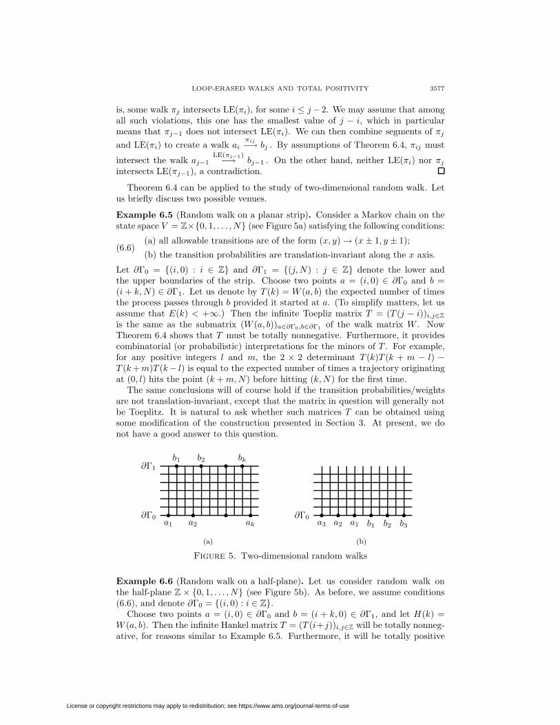
Example 6.5 (Random walk on a planar strip). Consider a Markov chain on thestate space V = Z×0, 1, . . . , N (see Figure 5a) satisfying the following conditions:

(a) all allowable transitions are of the form (x, y)→ (x ± 1, y ± 1);

(b) the transition probabilities are translation-invariant along the x axis.(6.6)

Let ∂Γ0 = (i, 0) : i ∈ Z and ∂Γ1 = (j,N) : j ∈ Z denote the lower andthe upper boundaries of the strip. Choose two points a = (i, 0) ∈ ∂Γ0 and b =(i + k,N) ∈ ∂Γ1. Let us denote by T (k) = W (a, b) the expected number of timesthe process passes through b provided it started at a. (To simplify matters, let usassume that E(k) < +∞.) Then the infinite Toepliz matrix T = (T (j − i))i,j∈Zis the same as the submatrix (W (a, b))a∈∂Γ0,b∈∂Γ1 of the walk matrix W . NowTheorem 6.4 shows that T must be totally nonnegative. Furthermore, it providescombinatorial (or probabilistic) interpretations for the minors of T . For example,for any positive integers l and m, the 2 × 2 determinant T (k)T (k + m − l) −T (k+m)T (k− l) is equal to the expected number of times a trajectory originatingat (0, l) hits the point (k +m,N) before hitting (k,N) for the first time.

The same conclusions will of course hold if the transition probabilities/weightsare not translation-invariant, except that the matrix in question will generally notbe Toeplitz. It is natural to ask whether such matrices T can be obtained usingsome modification of the construction presented in Section 3. At present, we donot have a good answer to this question.

s s s sa1 a2 ak

sb1 sb2 s sbk

∂Γ0

∂Γ1

(a)

s s s s s sa3 a2 a1 b1 b2 b3

∂Γ0

(b)

Figure 5. Two-dimensional random walks

Example 6.6 (Random walk on a half-plane). Let us consider random walk onthe half-plane Z × 0, 1, . . . , N (see Figure 5b). As before, we assume conditions(6.6), and denote ∂Γ0 = (i, 0) : i ∈ Z.

Choose two points a = (i, 0) ∈ ∂Γ0 and b = (i + k, 0) ∈ ∂Γ1, and let H(k) =W (a, b). Then the infinite Hankel matrix T = (T (i+j))i,j∈Z will be totally nonneg-ative, for reasons similar to Example 6.5. Furthermore, it will be totally positive


3578 SERGEY FOMIN

provided all transition probabilities between neighbouring states are positive. De-tails are left to the reader.

7. Minors of hitting matrices

The main goal of this section is to produce analogues of Theorems 6.1 and 6.4for hitting matrices. As before in Section 2, we assume that the vertex set V isarbitrarily partitioned into two disjoint subsets: the boundary ∂Γ and the interiorintΓ. Choose a pair of totally ordered subsets A = a1, . . . , ak ⊂ V and B =b1, . . . , bk ⊂ ∂Γ, and denote by XA,B = (X(ai, bj))i=1,...,k

j=1,...,kthe corresponding

hitting submatrix.Recall that LE(π) denotes the loop-erased part of a walk π.

Theorem 7.1. The minors of the hitting matrix are given by

det(XA,B) =∑σ∈Sk

sgn(σ)∑

a1π1−→ bσ(1), . . . , ak

πk−→ bσ(k)

w(π1) · · ·w(πk) ,(7.1)

where the first sum is over all permutations σ∈Sk, and the second sum runs overall families of walks π1, . . . , πk satisfying the following conditions:• πi has nonzero length, begins at ai, ends at bσ(i), and in the meantime does

not pass through any boundary vertices;• for any 1 ≤ i < j ≤ k, the walks πj and LE(πi) have no common vertices in

the interior of Γ.

Note that Theorem 7.1 reduces to Theorem 3.1 if the network is acyclic.Comparing to formula (4.4) (which has a narrower domain of applicability),

Theorem 7.1 has the advantage of “polynomiality:” the right-hand side of (7.1),unlike that of (4.4), is manifestly a formal power series in the edge weights. Thisfeature will be essential while extending the result to the continuous case.

Proof. This theorem can be proved by a direct argument similar to the one used inthe proof of Theorem 6.1. To save an effort, we will instead use a simple observationthat will reduce Theorem 7.1 to Theorem 6.1.

Let us define a new network Γ′ by splitting every boundary vertex b ∈ ∂Γ intoa source b′ and a sink b′′, converting all outgoing edges b→c into b′→c, redirectingall incoming edges a→b into a→b′′, and keeping the edge weights intact. Let ∂Γ′

and ∂Γ′′ be the sets of sources and sinks, respectively. Then the hitting matrixX of the original network Γ becomes a submatrix of the walk matrix W ′ of thetransformed network Γ′; more precisely, X(a, b) = W ′(a′, b′′) for a, b ∈ ∂Γ, whileX(a, b) = W ′(a, b′′) for a ∈ V \ ∂Γ and b ∈ ∂Γ. To complete the proof, it remainsto carefully reformulate the statement of Theorem 6.1 for Γ′ (with each ai ∈ ∂Γreplaced by a′i and each bj replaced by b′′j ) in terms of Γ.

The following analogue of Theorem 6.4 is a corollary of Theorem 7.1.

Theorem 7.2. Assume that the vertices a1, . . . , ak ∈ V and b1, . . . , bk ∈ ∂Γ havethe property that any walk from ai to bj through the interior of Γ intersects anysuch walk from ai′ , i′ > i, to bj′ , j′ < j, at a point in the interior. Then

det(XA,B) =∑

w(π1) · · ·w(πk) ,(7.2)

where the sum runs over all families of walks π1, . . . , πk satisfying the followingconditions:



• πi has nonzero length, begins at ai, ends at bi, and in the meantime does notpass through any boundary vertices;• for any 1≤ i<k, the walk πi+1 has no common vertices with the loop-erased

part of πi in the interior of Γ.In particular, if the edge weights are nonnegative, then the matrix XA,B is totallynonnegative.

The proof of Theorem 7.2 is similar to that of Theorem 6.4, and is omitted.

Example 7.3. In Example 2.4, let us verify Theorem 7.2. We have

det(XA,B) = (1 − q1q2q3)−2

∣∣∣∣∣∣∣∣ q4q5 q1q3q4q7

q1q2q5q6 q1q6q7

∣∣∣∣∣∣∣∣ = (1− q1q2q3)−1q1q4q5q6q7 .

On the other hand, the right-hand side of (7.2) is the product of X(a1, b1) =(1 − q1q2q3)−1q4q5 and the weight of the only walk a2

π2−→ b2 that does not in-tersect the only self-avoiding walk a1

π1−→ b1. This weight being equal to q1q6q7,Theorem 7.2 checks.

Hitting matrices of Markov chains. If the weights of a directed network aretransition probabilities (cf. Example 2.5), Theorem 7.2 has the following probabilis-tic interpretation.

As before, consider a Markov chain on the state space V with “boundary” ∂Γ ⊂V . The entries of the hitting matrix X are the hitting probabilities: X(a, b) is theprobability that b is the first boundary state hit by the process that originates at a.(Here and below in Theorem 7.4, a “hit” must occur after the clock is started. Inother words, if the process originates at a boundary state, it is not presumed to hitthe boundary right away.)

Theorem 7.4. Suppose that totally ordered subsets A = a1, . . . , ak ⊂ V andB = b1, . . . , bk ⊂ ∂Γ are such that any possible trajectory connecting ai to bjthrough intΓ intersects any trajectory connecting ai′ , i′ > i, to bj′ , j′ < j, ata point in intΓ. Then the minor det(XA,B) of the hitting matrix X is equal tothe probability that k independent trajectories π1, . . . , πk originating at a1, . . . , ak,respectively, will hit the boundary ∂Γ for the first time at the points b1, . . . , bk,respectively, and furthermore, the trajectory πi+1 will have no common verticeswith the loop-erased part of πi in the interior of Γ, for i = 1, . . . , k − 1.

In particular, det(XA,B) ≥ 0, and moreover the matrix XA,B is totally nonneg-ative.

To illustrate, the hitting matrices for two-dimensional random walks discussedin Examples 6.5 and 6.6 are totally nonnegative.

As an application of Theorem 7.4, we obtain another proof of total nonnegativityof response matrices of resistor networks (see Corollary 4.6).

Generalized hitting matrices. For a ∈ V and B ⊂ ∂Γ, let X(a,B) denotethe corresponding hitting probability; that is, X(a,B) is the probability that theprocess originating at a will first hit the boundary at some point b ∈ B. Using mul-tilinearity of the determinant, we obtain the following modification of Theorem 7.4.(Other theorems above can also be given similar analogues.)

Theorem 7.5. Assume that distinct states a1, . . . , ak ∈ V and disjoint subsetsB1, . . . , Bk ⊂ ∂Γ are such that any possible trajectory connecting ai to Bj intersects


3580 SERGEY FOMIN

any trajectory connecting ai′ , i′ > i, to Bj′ , j′ < j, at a point in intΓ. Then thedeterminant det(X(ai, Bj)) is nonnegative, and moreover the matrix (X(ai, Bj)) istotally nonnegative.

Moreover, det(X(ai, Bj)) is equal to the probability that k independent trajecto-ries π1, . . . , πk originating at a1, . . . , ak, respectively, will hit the boundary ∂Γ forthe first time at points which belong to B1, . . . , Bk, respectively, and furthermore,the trajectory πi+1 will have no common vertices with the loop-erased part of πi inthe interior of Γ, for i = 1, . . . , k − 1.

In order for the statement of Theorem 7.5 to make sense, the Markov processunder consideration does not have to be discrete. Although the technical detailsremain to be worked out, it is clear that by passing to a limit in a discrete approx-imation, Theorem 7.5 can be generalized to (non-isotropic) Brownian motions onplanar domains, or arbitrary simply connected Riemann manifolds with boundary,subject to technical assumptions. (See Figure 6.) The same type of argument canbe used to justify well-definedness of the quantities involved; notice that in orderto define a continuous analogue of the probability appearing in Theorem 7.5, wedo not need the notion of loop-erased Brownian motion. Instead, we discretize themodel, compute the probability, and then pass to a limit. One can further extendthese results to densities of the corresponding hitting distributions.

The rest of this section is devoted to a couple of characteristic applicationsinvolving Brownian motion.

s s sq qq q q q

B1

B2

B3

a1a2

a3

Figure 6. Theorem 7.5

Brownian motion in the quadrant with reflecting side. Let

Ω = (x, y) : x ≥ 0, y ≥ 0 ,and consider the Brownian motion in Ω which reflects in (bounces off) [the positivepart of] the x axis (see Figure 7a). The y half-axis is absorbing, i.e., the processstops once it reaches a state (0, y), y ≥ 0. This is equivalent to taking a Brownianmotion in the half-plane x ≥ 0 that stops upon hitting the y axis, and reflectingthe portions of it that go into the lower quadrant (x, y) : x ≥ 0, y < 0 over thex axis.

Let the process start at time t = 0 at a point (x, 0), x > 0 on the x axis. Itis classically known (see, e.g., [9, Section 1.9] for two different proofs) that theBrownian motion in half-plane hits the y axis for the first time at a point Y (x) thathas the Cauchy distribution with appropriate parameter. Taking absolute values,we conclude that our process in Ω induces the hitting distribution on the half-line(0, y) : y ≥ 0 which has the density

K(x, y) =2x

π(x2 + y2), y ≥ 0 .



6

-s sx1 x2

x

sy1

sy2

y

Ω

(a)

-

-s sx1 x2

x

sy1

sy2 y

Ω

(b)

Figure 7. Brownian motion in domains with reflecting sides

It follows from the general results above that the kernel K(x, y) is totally positive,i.e., any determinant of the form det(K(xi, yj)) with 0 < x1 < x2 < · · · and0 < y1 < y2 < · · · is positive. This result is not new. What seems to be new isthe interpretation we give to such determinants in terms of loop-erased walks. Toillustrate, let us fix 0 < x1 < x2, and consider two independent trajectories π1 andπ2 which start at points (x1, 0) and (x2, 0) and end up hitting the y axis at points(0, Y (x1)) and (0, Y (x2)), respectively. Assume that these two points are the points(0, y1) and (0, y2) with 0 < y1 < y2, but we do not know which trajectory hit whichof the two points. Then the conditional probability of the scenario Y (x1) = y1,Y (x2) = y2 is larger than that of Y (x1) = y2, Y (x2) = y1, and the difference ofthese conditional probabilities, which is given by

K(x1, y1)K(x2, y2)−K(x1, y2)K(x2, y1)K(x1, y1)K(x2, y2) +K(x1, y2)K(x2, y1)

,

is equal to the conditional probability that π2 did not hit the loop-erased part of π1 .(We repeat once again that the well-definedness of the loop-erased Brownian motiondoes not have to be justified in order for such probabilities to make perfect sense.)Computations show that∣∣∣∣∣∣∣∣ K(x1, y1) K(x1, y2)

K(x2, y1) K(x2, y2)

∣∣∣∣∣∣∣∣ =4x1x2(x2

2 − x21)(y2

2 − y21)

π2∏2i=1

∏2j=1(x2

i + y2j )

,

and therefore the conditional probability in question is given by the surprisinglysimple formula

P (π1 ∩ LE(π2) = ∅ | Y (x1), Y (x2)=y1, y2) =(x2

2 − x21)(y2

2 − y21)

(x21 + y2

2)(x22 + y2

1).(7.3)

If we do not condition on the locations of the hitting points (still keeping theinitial locations x1 < x2 fixed), then the probability that the trajectory π2 origi-nating at x2 will not intersect the loop-erased part of the trajectory π1 that startsat x1 (or a similar quantity with π1 and π2 interchanged) is equal to

P (Y (x1)<Y (x2))−P (Y (x1)≥Y (x2))=∫ ∞

0

∫ ∞y1

∣∣∣∣∣∣∣∣ K(x1, y1) K(x1, y2)K(x2, y1) K(x2, y2)

∣∣∣∣∣∣∣∣ dy2dy1 .

Computing the integral yields

P (π1 ∩ LE(π2) = ∅) = − 4π2

(Li2(−α) + Li2(1− α) + ln(α) ln(1 + α) +

π2

12

),


3582 SERGEY FOMIN

where α =x2

x1and Li2(t) =

∞∑n=1

tn

n2is the dilogarithm function. In particular, if

α =√

5+12 (so the initial locations x1 and x2 are in golden ratio), then we obtain,

using [4], the formula P (π1 ∩ LE(π2) = ∅) = 13 −

6π2

(ln(√

5+12 )

)2.

Brownian motion in a strip with reflecting side. In this example, we let

Ω = (x, y) : x ∈ R, 0 ≤ y ≤ 1and consider the Brownian motion in Ω which is reflecting in the x axis (see Fig-ure 7b). The process begins at a point (x0, 0) on the x axis and stops when it hitsthe line y = 1.

Standard computations (employing either conformal invariance of Brownian mo-tion or the reflection principle) yield the well-known formula for the hitting density:

K(x0, x0 + x) =1

eπx2 + e−

πx2

=1

2 cosh(πx2 ).

Thus K is a totally positive translation-invariant kernel; equivalently, the function

K(x) =1

2 cosh(πx2 )is a Polya frequency function. This particular example of a

PF function is of course well known; see, e.g., Karlin [13, § 7.1, example (b)]. Thecomputation of probabilities related to loop-erased walks in this model is omitted.

References

1. I. Benjamini, R. Lyons, Y. Peres, and O. Schramm, Uniform spanning forests, Ann. Probab.,to appear.

2. W. Bohm and S. G. Mohanty, On the Karlin-McGregor theorem and applications, Ann. Appl.Probab. 7 (1997), 314–325. MR 98g:60131

3. B. Bollobas, Modern graph theory, Springer-Verlag, New York, 1998. MR 99h:050014. J. M. Borwein, D. M. Bradley, D. J. Broadhurst, and P. Lisonek, Special values of multiple

polylogarithms, Trans. Amer. Math. Soc., to appear.5. Y. Colin de Verdiere, Reseaux electriques planaires, Prepublications de l’Institut Fourier 225

(1992), 1–20.6. E. Curtis, D. V. Ingerman, and J. Morrow. Circular planar graphs and resistor networks,

Linear Algebra Appl. 283 (1998), 115–150. MR 99k:050967. E. Curtis, E. Mooers, and J. Morrow, Finding the conductors in circular networks from bound-

ary measurements, RAIRO Model. Math. Anal. Numer. 28 (1994), 781–814. MR 96i:651108. P. G. Doyle and J. L. Snell, Random walks and electric networks, Math. Assoc. of America,

1984. MR 89a:940239. R. Durrett, Brownian motion and martingales in analysis, Wadsworth, 1984. MR 87a:60054

10. S. Fomin and A. Zelevinsky, Total positivity: tests and parametrizations, Math. Intelligencer22 (2000), no. 1, 23–33. MR 2001b:22014

11. F. R. Gantmacher and M. G. Krein, Oszillationsmatrizen, Oszillationskerne und kleineSchwingungen mechanischer Systeme, Akademie-Verlag, Berlin, 1960. MR 22:5161 (Russianedition: Moscow-Leningrad, 1950. MR 14:178)

12. D. V. Ingerman, Discrete and continuous inverse boundary problems on a disk, Ph.D. thesis,University of Washington, 1997.

13. S. Karlin, Total positivity, Stanford University Press, 1968. MR 37:566714. S. Karlin and G. McGregor, Coincidence probabilities, Pacific J. Math. 9 (1959), 1141–1164.

MR 22:5072

15. G. Lawler, Intersections of random walks, Birkhauser, 1991. MR 92f:6012216. B. Lindstrom, On the vector representations of induced matroids, Bull. London Math. Soc. 5

(1973), 85-90. MR 49:9517. A. A. Milne, The house at Pooh corner, E. P. Dutton & Co., 1928 ff.


http://www.ams.org/mathscinet-getitem?mr=98g:60131

http://www.ams.org/mathscinet-getitem?mr=99h:05001

http://www.ams.org/mathscinet-getitem?mr=99k:05096

http://www.ams.org/mathscinet-getitem?mr=96i:65110

http://www.ams.org/mathscinet-getitem?mr=89a:94023


http://www.ams.org/mathscinet-getitem?mr=2001b:22014

http://www.ams.org/mathscinet-getitem?mr=22:5161




http://www.ams.org/mathscinet-getitem?mr=92f:60122



18. R. Pemantle, Choosing a spanning tree for the integer lattice uniformly, Ann. Probab. 19(1991), 1559–1574. MR 92g:60014

19. J. G. Propp and D. B. Wilson, How to Get a Perfectly Random Sample from a Generic MarkovChain and Generate a Random Spanning Tree of a Directed Graph, J. Algorithms 27 (1998),170–217. MR 99g:60116

20. F. Spitzer, Principles of random walk, Van Nostrand, 1964. MR 30:152121. R. P. Stanley, Enumerative combinatorics, vol. 1, 2d ed., Cambridge Univ. Press, 1997. MR

98a:0500122. D B. Wilson, Generating random spanning trees more quickly than the cover time, Proceedings

of the Twenty-Eighth Annual ACM Symposium on the Theory of Computing, 296–303, 1996.MR 97g:68005

Department of Mathematics, University of Michigan, Ann Arbor, Michigan 48109

E-mail address: [email protected]







introduction · 3564 sergey fomin up where; neither do we know how much time it took for each one...

Documents