3.5-1 routing and deadlock 3.5-1 · therefore network deadlock free. note: theorem speciﬂed...

3.5-1 3.5-1Routing and Deadlock

Routing would be easy . . .

. . . were it not for possible deadlock.

Topics For This Set:

• Routing definitions.

• Deadlock definitions.

• Resource dependencies.

• Acyclic deadlock free routing techniques.

• Virtual channels and acyclic deadlock free routing techniques.

• Cyclic deadlock free routing techniques

3.5-1 EE 7725 Lecture Transparency. Formatted 12:19, 8 June 2001 from lsli03˙5. 3.5-1

3.5-2 3.5-2Routing Definitions

Oblivious Routing

Path uniquely defined by source and destination.

I.e., ignore network congestion, etc. when choosing path.

Adaptive Routing

Path chosen based on network conditions (and source and desto too, of course).

Path might be changed within network to avoid congestion.

Unrestricted (a.k.a., Fully Adaptive) Routing

Adaptive routing in which any neighboring node can be used in path.

Minimal Routing

Each link takes message closer to destination.

In non-minimal routing path might lead away from desto . . .

. . . presumably to avoid congestion.


3.5-3 3.5-3Comparison of Routings

Minimality (Length of Path)

Adaptive routing can be minimal or non-minimal.

Oblivious routing is usually minimal.

In-Order Delivery

Needed for certain systems, such as cache-coherence protocols.

Oblivious routing guarantees in-order message delivery.

Adaptive routing cannot normally do this.


3.5-4 3.5-4

Routing Function

Returns node outputs a message can take based on node input used and destination.

R | Q × 〈N〉 → Q?

where Q is the set of all links (link buffers) in the network [current location],

〈N〉 is the set of all network outputs (usually nodes), [destination],

and Q? is the set of all possible subsets of Q [possible node outputs].

For oblivious routing, |R(q, d)| = 1,

where q ∈ Q is a link buffer

and d ∈ 〈N〉 is a destination.

For unrestricted routing, |R(q, d)| = δ,

where δ is the number of links (or virtual channels) leaving the cell.

Note: The routing function specifies which links could be taken . . .

. . . another function is needed to choose among these.

That other function will not be discussed here.


3.5-5 3.5-5Deadlock Definitions

Deadlock

A situation where there are activities (e.g., messages) . . .

. . . each waiting for another to finish something.

Since a waiting activity cannot finish, deadlock is forever1.

Livelock

A situation where a message can move from node to node . . .

. . . but will never get to its destination.

Yes, it happens.

Starvation

The fate of a contender for a resource . . .

. . . that is never granted the resource . . .

. . . due to an unfair contention-resolution policy.

Livelock and starvation will not be covered further.

1 Unless the waiting activity is somehow aborted.


3.5-6 3.5-6Handling Deadlock

Clear existing deadlock.Okay approach.

Guarantee that deadlock never happens.Better approach.


3.5-7 3.5-7Clearing Deadlock

Detecting deadlock for certain too time consuming.

Instead guess:

If nothing moves for some amount of time, assume deadlock.

Possible Implementation: Compression-Free Routing

Use wormhole routing with single-slot buffers.

Insure the shortest message is longer than longest path.(Messages that would be too short are padded.)

Sending node starts a countdown timer if message stops.

If timer expires and message hasn’t moved, assume deadlock . . .

. . . and kill the message.

Retransmit, possibly after a delay and possibly on another path.


3.5-8 3.5-8Compression-Free Routing

Advantages

Easy to implement: sender can directly detect possible deadlock.

Fully adaptive.

Disadvantage

If deadlock occurs frequently efficiency suffers (due to timer delay).


3.5-9 3.5-9Resource Dependencies

Resource

Something needed to do something.

E.g., link, buffer.

Resource Dependence

A relationship between two resources indicating . . .

. . . the first may not be available . . .

. . . until after the second is available.

(That is, the first needs the second to finish what it’s doing.)

Network Resources

Links, Buffers, Crossbar Outputs

Could use all three, but sufficient to consider only links.

Link resources equivalent to buffers when links connected to buffers.

Treat bidirectional link as two links.


3.5-10 3.5-10

Network Dependence Example

Link 〈1, 1〉 dependent on links 〈2, 0〉, 〈2, 1〉, and 〈2, 2〉..If messages not allowed to reverse direction, 〈1, 1〉 not dependent on 〈2, 3〉.

<1,1>

<2,0>

<2,2>

<2,1>

<2,3>


3.5-11 3.5-11

Link Dependence

In a given network using a given routing algorithm . . .

. . . there is a dependence between link A and B . . .

. . . if they are incident to the same node . . .

. . . and a message can move from link A through the node to B . . .

. . . using the routing algorithm.


3.5-12 3.5-12

Dependence Graph

Used for analyzing deadlock.

A dependence graph consists of a vertex for each resource . . .

. . . and a directed edge from vertex A to B . . .

. . . if A is dependent on B.

Network Dependence Graph

Vertices are (usually) links.

Links to processors are sometimes included.

Message using link to processor will never block.


3.5-13 3.5-13

Example Dependence Graph

<1,1>

<2,0>

<2,2>

<2,1>

<2,3>

<1,1>

<2,0>

<2,2>

<2,1>


3.5-14 3.5-14Deadlock and Dependence Graphs

Consider:

1

23

<1,0>

<2,0>

<3,0>

<1,0>

<2,0>

<3,0>

Link

Node

Dependence

Network Dep. Graph

No message could move if all buffers were full.

(A packet cannot move into a full buffer.)

Relationship with dependence graph clear.


3.5-15 3.5-15

Deadlock Theorem

If a network’s dependence graph is acyclic, it’s deadlock-free.

Proof Setup

Number vertices such that . . .

. . . if there’s a dependence from A to B . . .

. . . then A has a higher number than B.

(All acyclic graphs can be numbered this way.)


3.5-16 3.5-16

Deadlock Theorem Proof Plan

Mark as many deadlock-free links as possible.

If all links marked, network deadlock free.

Proof

All links to processors deadlock free (can’t block).

All links dependent only on links to processors are deadlock free.

Consider lowest-numbered non-processor link.

It must be deadlock free since it only depends on processor links.

Then the same must be true for second-lowest-numbered non-proc link.

By induction on these link numbers, all links are deadlock free.

Therefore network deadlock free.

Note:

Theorem specified acyclicness as a sufficient but not a necessary condition.

So, even if a network’s dependence graph is cyclic, it still may be deadlock-free.


3.5-17 3.5-17

Acyclic Dependence Example: Dimension-Order Mesh Routing

Route mesh in dimension order. Is minimal (good) but oblivious (bad).

0 1

2 3

<0,1>

<0,2><1,3>

<1,2>

<3,0>

<3,3>

<2,1><2,0>

<0,1>

<1,2>

<3,3>

<2,0>

<0,2>

<1,3>

<3,0>

<2,1>

<0,1>

<1,2>

<3,3>

<2,0>

<0,2>

<1,3>

<3,0>

<2,1>

Network Unrestricted Routing

Dependence Graph

Dim-Order Routing

Dependence Graph


3.5-18 3.5-18

Dimension-Order Routing and KNC

Deadlock still possible.

E.g., 1-D network, messages from i to i + 1 mod N for all i ∈ 〈N〉.

Virtual Channel Motivation

Will show that deadlock in KNCs could be avoided by adding links . . .

. . . but that’s expensive.

Same deadlock freedom obtained using virtual channels (virtual links).


3.5-19 3.5-19Virtual Channels

Dally & Sietz, IEEE ToC, vol. C-36, no. 5, pp. 547-553, May 1987.

Virtual Channel (VC)A connection between two nodes which can be used as a single link . . .

. . . but which physically must share a link with other virtual channels.

To routing and flow control mechanisms, virtual channel equivalent to link.

Since multiple virtual channels can share a single link . . .

. . . bandwidth of each virtual channel less than link.


3.5-20 3.5-20

Virtual Channel Implementation

Separate buffers for each virtual channel.

Link

(Physical

Channel)

Buffer for

VC 1

Buffer for

VC 2

Carries

Two Virtual

Channels

Virtual Channel Key Feature

A message blocked in one virtual channel . . .

. . . does not prevent message in any other virtual channel from using link.


3.5-21 3.5-21

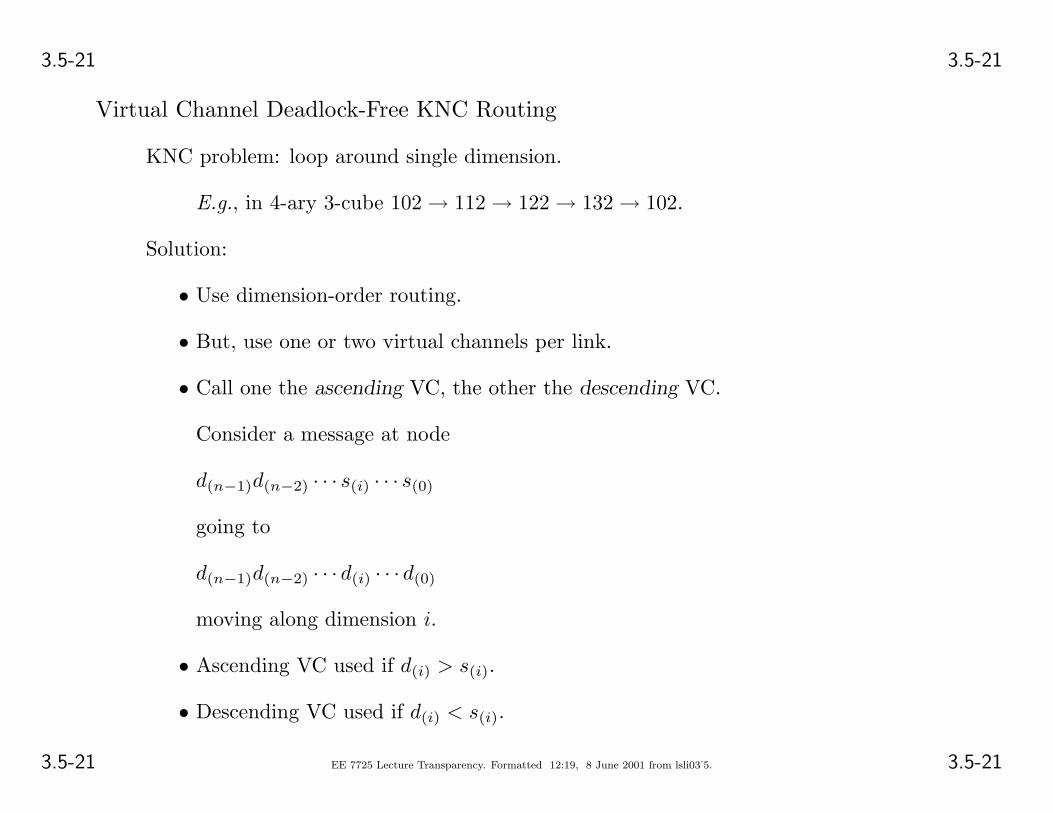
Virtual Channel Deadlock-Free KNC Routing

KNC problem: loop around single dimension.

E.g., in 4-ary 3-cube 102 → 112 → 122 → 132 → 102.

Solution:

• Use dimension-order routing.

• But, use one or two virtual channels per link.

• Call one the ascending VC, the other the descending VC.

Consider a message at node

d(n−1)d(n−2) · · · s(i) · · · s(0)

going to

d(n−1)d(n−2) · · · d(i) · · · d(0)

moving along dimension i.

• Ascending VC used if d(i) > s(i).

• Descending VC used if d(i) < s(i).


3.5-22 3.5-22

Note: some links need only one virtual channel.

Virtual Channel Deadlock-Free KNC Routing Example

Avoiding deadlock in 5-ary 1-cube:

0 1 2 3 4

asc

des des des des

asc asc

asc

(Virtual channels shown.)

0

1 2 3

4

asc

des des des des

asc asc

asc

321


3.5-23 3.5-23

Dimension-Order Routing Drawback: Non-Adaptive (Oblivious)

No way to avoid congestion.

Adding choices to routing complicates dependence graph . . .

. . . and complicates acyclic proofs.

Tool to help analyze dependence graphs: Turn Model


3.5-24 3.5-24Turn Model

Glass & Ni, JACM, vol. 41, no. 5, September 1994, pp. 874-902.

Tool to help visualize possible cycles in dependence graphs.

Consider networks with some translational symmetry.

(The network could be constructed using regularly placed duplicates of a singlenode and some incident links, with a possible extra step for adding special[e.g.,wraparound] connections.)

Define a turn to be a pair of links incident to the same node.

Idea:

• Consider all possible turns (dimension changes) in network.

• Ignore pairs of links in same direction (0◦ turn).

• Ignore pairs of links in opposite direction (180◦ turn).

• Eliminate just enough turns to break cycles.

It’s easy to break obvious cycles.

Proving that all cycles broken still difficult.


3.5-25 3.5-25

Turn Model Example

All turns in 2-D mesh:

Turns in dimension-order routing:

Note that could have kept more turns!

Turns in north-last routing:

Note that message sometimes can avoid congestion.

Several other adaptive 2-D mesh routing schemes are possible.


3.5-26 3.5-26

Turn Model with Virtual Channels.

A topological direction of a VC is the direction of the physical link.

For turn model, each of a link’s VCs go in a different virtual direction.

Analyze as non-VC turn model.

Note that 0◦ topological-direction turn not necessarily 0◦ direction turn.


3.5-27 3.5-27

Applying Turn Model to KNC

Method One: Virtual Network

Add virtual channels to create non-wraparound network.

Apply turn model to that network.

Method Two: Improvise

Start with a turn-model analysis, ignoring wraparound connections.

Add wraparound links, modifying turn-model rules.

(You either love it or you hate it.)


3.5-28 3.5-28Deadlock-Free Cyclic Routing

Wormhole: Duato, IEEE TPDS, vol. 4, no. 12, pp. 1230-1331, December 1993.Store & Forward: Duato, IEEE TPDS, vol. 7, no. 8, pp. 841-854, August 1996.

Deadlock-Free Cyclic Routing

Idea: Guarantee cycle-free path to desto . . .

. . . though cycles exist on other paths in dependence graph.

Method: Choose VC and routing so that a subgraph is cycle free.

Tricky for several reasons.

HOL blocking could deadlock messages . . .

. . . at a node having a deadlock-free link.

Must consider dependencies in subgraph due to messages arriving from outside.

Can be used to design highly adaptive routing algorithm.

Theory and techniques not covered.


3.5-1 routing and deadlock 3.5-1 · therefore network deadlock free. note: theorem speciﬂed...

Documents