NASA/CR-2013-217922

Vandenberg Air Force Base Pressure Gradient Wind Study Jaclyn A. Shafer ENSCO, Inc., Cocoa Beach, Florida NASA Applied Meteorology Unit, Kennedy Space Center, Florida

September 2013

NASA STI Program ... in Profile

Since its founding, NASA has been dedicated to the advancement of aeronautics and space science. The NASA scientific and technical information (STI) program plays a key part in helping NASA maintain this important role. The NASA STI program operates under the auspices of the Agency Chief Information Officer. It collects, organizes, provides for archiving, and disseminates NASA’s STI. The NASA STI program provides access to the NASA Aeronautics and Space Database and its public interface, the NASA Technical Reports Server, thus providing one of the largest collections of aeronautical and space science STI in the world. Results are published in both non-NASA channels and by NASA in the NASA STI Report Series, which includes the following report types: • TECHNICAL PUBLICATION. Reports of

completed research or a major significant phase of research that present the results of NASA Programs and include extensive data or theoretical analysis. Includes compilations of significant scientific and technical data and information deemed to be of continuing reference value. NASA counter-part of peer-reviewed formal professional papers but has less stringent limitations on manuscript length and extent of graphic presentations.

• TECHNICAL MEMORANDUM.

Scientific and technical findings that are preliminary or of specialized interest, e.g., quick release reports, working papers, and bibliographies that contain minimal annotation. Does not contain extensive analysis.

• CONTRACTOR REPORT. Scientific and

technical findings by NASA-sponsored contractors and grantees.

• CONFERENCE PUBLICATION. Collected papers from scientific and technical conferences, symposia, seminars, or other meetings sponsored or co-sponsored by NASA.

• SPECIAL PUBLICATION. Scientific,

technical, or historical information from NASA programs, projects, and missions, often concerned with subjects having substantial public interest.

• TECHNICAL TRANSLATION.

English-language translations of foreign scientific and technical material pertinent to NASA’s mission.

Specialized services also include organizing and publishing research results, distributing specialized research announcements and feeds, providing information desk and personal search support, and enabling data exchange services. For more information about the NASA STI program, see the following: • Access the NASA STI program home page

at http://www.sti.nasa.gov • E-mail your question to help@sti.nasa.gov • Fax your question to the NASA STI

Information Desk at 443-757-5803 • Phone the NASA STI Information Desk at

443-757-5802 • Write to: STI Information Desk NASA Center for AeroSpace Information 7115 Standard Drive Hanover, MD 21076-1320

2

NASA/CR-2013-217922

Vandenberg Air Force Base Pressure Gradient Wind Study Jaclyn A. Shafer ENSCO, Inc., Cocoa Beach, Florida NASA Applied Meteorology Unit, Kennedy Space Center, Florida National Aeronautics and Space Administration Kennedy Space Center Kennedy Space Center, FL 32899-0001

September 2013

Acknowledgements The author would like to thank Dr. William Bauman, Ms. Winifred Crawford, and Dr. Leela

Watson of the Applied Meteorology Unit, Dr. Lisa Huddleston of the Kennedy Space Center Weather Office and Mr. William Roeder of the 45th Weather Squadron for lending their time, data management, and statistical expertise to this task. Mr. Tyler Brock of the 30th Operational Support Squadron and Mr. Ben Kenyon of WROCI/Indyne also played a significant role providing historical Vandenberg Air Force Base tower network data for this task.

Available from:

NASA Center for AeroSpace Information 7115 Standard Drive

Hanover, MD 21076-1320 443-757-5802

This report is also available in electronic form at

http://science.ksc.nasa.gov/amu/

2

Executive Summary Customer: Launch Services Program (LSP)

Warning category winds can adversely impact day-to-day space lift operations at Vandenberg Air Force Base (VAFB) in California. NASA’s LSP and other programs at VAFB use wind forecasts issued by the 30th Operational Support Squadron Weather Flight (30 OSSWF) to determine if they need to limit activities or protect property such as a launch vehicle. For example, winds ≥ 30 kt can affect Delta II vehicle transport to the launch pad, Delta IV stage II attitude control system tank load, and other critical operations. The 30 OSSWF uses the mean sea level pressure (MSLP) from seven regional observing stations to determine the pressure difference (dP) as a guide to forecast surface wind speed at VAFB. Their current method uses an Excel-based tool that is manually intensive and does not contain an objective relationship between peak wind and dP. They require a more objective and automated capability to help them forecast the onset and duration of warning category winds to enhance the safety of their customers’ operations. The 30 OSSWF tasked the Applied Meteorology Unit (AMU) to develop an automated Excel graphical user interface (GUI) that uses the pressure observations at specific observing stations under different synoptic regimes to aid forecasters in determining when wind warnings should be issued. The AMU suggested that the tool use pressure gradients (PG) instead of dP as it is a more accurate indicator of local wind speed, and the 30 OSSWF agreed. Development of such a tool would require that solid relationships exist between the peak wind speed and the PG of one or more station pairs.

In order to determine past high wind events on VAFB and compare the local PGs at the time, the AMU required historical wind data from the VAFB wind tower network and MSLP observations from weather observing stations used operationally by the 30 OSSWF. The 30 OSSWF delivered all available data from their 26 VAFB wind towers from October 2007 – November 2012. The AMU processed the observations to develop a database containing maximum hourly peak winds for each tower and day in the dataset. Meanwhile, the 45th Weather Squadron (45 WS) obtained historical MSLP observations data from the 14th Weather Squadron (14 WS). Once received, the AMU developed an MSLP database containing hourly observations from each station. These observations were organized by synoptic regime and the hourly PGs for each station pair were calculated.

To better understand the relationship between peak wind and PG at VAFB, the AMU created a series of graphs plotting PG and maximum peak wind (MPW) versus time for each of the synoptic regimes. These graphs were created for four days in each synoptic regime, each day representing a different time of the year in order to have a diverse collection of case studies. The initial review of PGs and MPW did not yield a clear qualitative relationship between the two variables regardless of the time of year or synoptic regime. Given this result, the AMU calculated correlation coefficients between PG and MPW to quantitatively measure the relationship between them using the entire 2007-2012 database. Most of the Pearson correlation coefficient (PCC) values ranged between -0.1 and 0.4 with occasional outliers. Given PCC indicates no relationship when it is equal to zero, these statistics confirm a weak relationship between PG and MPW at VAFB. Based on the PG evaluation and calculated PCC values, the AMU was unable to determine PG thresholds for the station pairs and therefore did not automate the 30 OSSWF wind tool. This report provides a description of the data used and the results of the analyses to show the lack of relationship between PG and peak winds at VAFB.

2

Table of Contents Executive Summary ................................................................................................................... 2

Table of Contents ....................................................................................................................... 3

List of Figures ............................................................................................................................ 4

List of Tables ............................................................................................................................. 5

1 Introduction .......................................................................................................................... 6

2 Data Acquisition and Processing .......................................................................................... 7

2.1 VAFB Synoptic Regimes .............................................................................................. 7 2.2 VAFB Wind Tower Data................................................................................................ 9 2.3 Regional Observing Station Data ................................................................................ 11

3 Data Analysis ......................................................................................................................13

3.1 Pressure Gradient Evaluation: Full Base .................................................................... 13 3.2 Pressure Gradient Evaluation: North and South Base ................................................ 16 3.3 Correlation .................................................................................................................. 21

4 Summary .............................................................................................................................24

List of Acronyms .......................................................................................................................26

3

List of Figures Figure 1. Charts depicting the synoptic conditions for each of the regimes included in this

study. The red solid line indicates the location of the PFJ. The blue H indicates a high pressure area, the red L indicates a low pressure area. .................................... 8

Figure 2. Locations of the 26 wind towers in the VAFB network (KVBG in Figure 3). ..............10

Figure 3. Locations of the seven observing stations used to calculate PG. KVBG is VAFB. ...11

Figure 4. Example PG/MPW versus time graph for the ≥ 40 kt wind event on 14 July 2011 with a CH regime. The MPW values are on the left y-axis, the PG values between all the station pairs in the legend are on the right y-axis, and the time in UTC is on the x-axis. .........................................................................................................................14

Figure 5. Same as Figure 4 except ABS(PG) replaces PG on the right y-axis. .......................14

Figure 6. Same as Figure 5, except for 25 January 2008 in the UT regime. ...........................15

Figure 7. Same as Figure 5, except for 4 November 2008 in the NPL regime. .......................16

Figure 8. All VAFB wind towers designated as North Base (yellow) and South Base (light blue). .......................................................................................................................17

Figure 9. Example ABS(PG)/MPW versus time graph with PH regime. The MPW is on the left y-axis, the ABS(PG) is on the right y-axis, and time is on the x-axis. .......................18

Figure 10. Same as Figure 9 except for NB/SB ABS(PG)/MPW. NB-MPW are the solid black line with diamonds, the SB-MPW are the dashed line with circles. ...........................18

Figure 11. Same as Figure 10 except for 22 August 2010. .......................................................19

Figure 12. Same as Figure 10 except for 18 July 2011 and for a CL regime. ............................20

Figure 13. ABS(PG) PCC versus synoptic regime for the full base from 2007-2012. The solid black line highlights where PCC equals zero. The PCC is on the y-axis and the synoptic regime on the x-axis. The “ALL” category on the x-axis includes all of the days in the 2007-2012 database regardless of synoptic regime and the solid black horizontal line highlights where PCC equals zero. ...................................................22

Figure 14. Same as Figure 13 except for NB towers. ................................................................22

Figure 15. Same as Figure 13 except for SB towers. ................................................................23

Figure 16. Same as Figure 13 except for dP. ............................................................................24

4

List of Tables Table 1. Number of days with peak winds ≥ 40 kt for each synoptic regime. .........................10

Table 2. List of the 30 OSSWF-identified station pairs and distance (km) between them used in the PG calculations. The station pairs below the green line were added by the AMU. .......................................................................................................................12

Table 3. List of the 30 OSSWF towers classified by NB/SB and their respective elevations in feet. .........................................................................................................................21

5

1 Introduction Warning category winds can adversely impact day-to-day space lift operations at

Vandenberg Air Force Base (VAFB) in California. NASA’s Launch Services Program (LSP) and other programs at VAFB use wind forecasts issued by the 30th Operational Support Squadron Weather Flight (30 OSSWF) to determine if they need to limit activities or protect property such as a launch vehicle. For example, winds ≥ 30 kt can affect Delta II vehicle transport to the launch pad, Delta IV stage II attitude control system tank load, and other critical operations. The 30th Operational Support Squadron Weather Flight (30 OSSWF) at VAFB uses the mean sea level pressure (MSLP) from seven regional observing stations to determine the pressure difference (dP) as a guide to forecast surface wind speed at VAFB. Their current method uses an Excel-based tool that is manually intensive and does not contain an objective relationship between peak wind and dP. They require a more objective and automated capability to help them forecast the onset and duration of warning category winds to enhance the safety of their customers’ operations. The 30 OSSWF tasked the Applied Meteorology Unit (AMU) to develop an automated Excel graphical user interface (GUI) that uses the pressure observations at specific observing stations under different synoptic regimes to aid forecasters in determining when wind warnings should be issued.

As stated previously, the 30 OSSWF forecasters use dP as their guide for forecasting peak winds. The AMU suggested that the tool use pressure gradients (PG) instead of dP as it is a more accurate indicator of local wind speed, and the 30 OSSWF agreed. Therefore, the AMU used the PG between the regional observing stations and VAFB wind tower data, both stratified by synoptic-scale flow regimes, to determine relationships between PG and peak winds at VAFB.

The goal of this task, then, was to develop an automated tool that would use relationships between PG values and peak winds to determine PG thresholds under different synoptic regimes that would provide objective peak wind forecast guidance to the 30 OSSWF. Development of such a tool would require that solid relationships exist between the peak wind speed and the PG of one or more station pairs. The AMU conducted subjective and objective analyses to discern such relationships, but found there were none. As a result, the requested GUI could not be developed. This report provides a description of the data used and the results of the analyses to show the lack of relationship between PG and peak winds at VAFB.

6

2 Data Acquisition and Processing The goal of this task as stated in the previous section required identification of past high

wind events and calculating the local PG values between regional observing station pairs under different synoptic regimes at the times of those peak winds. These two parameters were used to identify PG thresholds related to the occurrence of the peak winds. In order to identify past high wind events on VAFB and compare the PGs between observing stations at the same time, the AMU required historical wind data from the VAFB wind tower network and MSLP observations from weather observing stations used operationally by the 30 OSSWF. The AMU acquired and processed VAFB wind tower network data and MSLP observations from seven 30 OSSWF-identified weather observing stations in the period 2007–2012.

2.1 VAFB Synoptic Regimes Overall, there are 11 synoptic regimes that affect the weather at VAFB. For the days

included in this study, seven of them were observed. Each regime is summarized below and illustrated in Figure 1.

Pacific High (PH): This is a semi-permanent summer regime that develops in late May and lasts through late September. It may extend beyond the standard time frame when the upper-level pattern remains unchanged for extended periods of time. The high is generally recognized as a well-established surface feature and is located hundreds of miles off the California coast.

North Pacific Low (NPL): This is most recognizable in fall through winter low pressure regimes that affect California. It is usually quick moving and highly dependent on the speed and position of the polar front jet (PFJ). This feature is usually very cold, originates from the Gulf of Alaska and is evident from the surface up to 200 mb. Depending on dynamics and moisture content, thunderstorms are possible.

North Pacific High (NPH): This regime typically begins as a post-frontal ridge that extends from the Pacific into the western portion of the continental United States. It typically follows the NPL regime and is most common through the early fall to late spring.

California High (CH): This is not a typical high pressure regime but, when present, the surface feature is easily recognized off the northern coast of California during the fall to early spring. Northwest flow is dominant in this system and often brings stronger winds to VAFB.

California Low (CL): This is the most powerful system common to the West Coast because it is located farther south and exhibits tremendous upper-level support for widespread precipitation and severe weather. It is most common during the winter to early spring south of 42° N. Cooler mid-level temperatures are common with these systems and lead to thunderstorm development. These systems usually move quickly and are followed by the CH regime.

Upper Trough (UT): This is defined by an upper-level feature that becomes more barotropic with time and cut off from the main portion of the PFJ. These features can be distinguished from 200–300 mb down to the surface before they dissipate. When they move over California they bring unsettled weather with the strongest winds around the base of the low. These systems bring the best chance for thunderstorm development at VAFB.

Great Basin High (GBH): The Great Basin is defined as the area between the Sierra Nevada, Cascades and Rocky Mountains. This high pressure system is caused by cold air that becomes trapped by the Rocky Mountains on the east and the Sierra Nevada Mountains on the west. The GBH remains a shallow feature that is mostly confined to 700 mb and below. This system brings dry conditions, larger temperature fluctuations and generally clear skies at VAFB.

7

Figure 1. Charts depicting the synoptic conditions for each of the regimes included in this study. The red solid line indicates the location of the PFJ. The blue H indicates a high pressure area, the red L indicates a low pressure area.

8

2.2 VAFB Wind Tower Data The 30 OSSWF delivered all available data from their 26 VAFB wind towers (Figure 2) for

the October 2007–November 2012 time period. Each tower reports observations at three different sensor heights (2, 4 and 16 m) with the exception of tower 0087, which only had observations at 16 m. Since the 30 OSSWF verifies their wind warnings from the 4 m sensors, the AMU identified all 4-m one-minute average peak wind observations and confirmed all values fell within valid meteorological ranges. The hourly averages at each tower were then calculated using Perl scripts.

The AMU filtered the wind tower data into a database containing maximum hourly peak winds for each tower and day in the period, and then determined all days where peak winds ≥ 30 kt were observed. As previously mentioned, the 30 OSSWF agreed to organize the AMU-identified high wind event days by synoptic regime. Considering the number of ≥ 30 kt peak wind days was over 1,200, the 30 OSSWF requested the peak wind threshold be increased to ≥ 40 kt to reduce the number of days in the database. Per this request, the AMU identified all days where peak winds ≥ 40 kt were observed, 745 in all, and provided a list of these dates to the 30 OSSWF. Table 1 shows the number of ≥ 40 kt days in each of the synoptic regimes described in the previous section.

9

Figure 2. Locations of the 26 wind towers in the VAFB network (KVBG in Figure 3).

Table 1. Number of days with peak winds ≥ 40 kt for each synoptic regime.

Synoptic Regime Number of ≥ 40 kt days

Pacific High (PH) 141 North Pacific Low (NPL) 153 North Pacific High (NPH) 141 California High (CH) 81 California Low (CL) 81 Upper Trough (UT) 64 Great Basic High (GBH) 84

10

2.3 Regional Observing Station Data In addition to the wind tower data, the AMU also required historical MSLP observations. The

45th Weather Squadron (45 WS) obtained the MSLP observations from the seven weather stations identified by 30 OSSWF for calculating PGs (Figure 3) from the 14th Weather Squadron (14 WS). Once received, the AMU wrote Perl scripts to develop an MSLP database containing hourly observations from each station on the days when peak winds ≥ 40 kt were observed in the VAFB wind tower network. These observations were stratified by the synoptic regimes described previously, and the hourly PGs for each station pair were calculated in Microsoft Excel. The 30 OSSWF station pairs, distance between stations, and PG formula are in Table 2. The two station pairs listed below the green line are additional pairs the AMU included to further evaluate the relationship between peak wind and PG at VAFB.

Figure 3. Locations of the seven observing stations used to calculate PG. KVBG is VAFB.

11

Table 2. List of the 30 OSSWF-identified station pairs and distance (km) between them used in the PG calculations. The station pairs below the green line were added by the AMU.

Station Pair Distance (km)

KVBG – KBFL 159.0 KBFL – KLAS 359.6 KVBG – KLAS 514.4 KACV – KSFO 402.1 KSFO – KPRB 266.7 KPRB – KVBG 104.1 KVBG – KLAX 218.5 KACV – KPRB 663.3 KPRB – KLAX 279.4 KACV – KVBG 759.6 KSFO – KVBG 358.5 KACV – KLAX 929.6

KPRB – KLAS 495.3 KLAX – KLAS 380.0

Pressure Gradient (PG) formula:

𝑃𝐺 = �𝑑𝑃𝐷� ∗ 100

Where: dP = Pressure difference (mb) between two stations

D = Distance (km) between two stations

12

3 Data Analysis The AMU analyzed peak wind and PG values stratified by synoptic regime subjectively and

objectively to determine if relationships existed between them. If a relationship could be found, the AMU would then determine PG thresholds that could be used to forecast warning-level winds on VAFB.

3.1 Pressure Gradient Evaluation: Full Base In order to better understand the relationship between peak wind and PG at VAFB, the AMU

created a series of graphs plotting PG and maximum peak wind (MPW) versus time for each of the synoptic regimes. The MPW was the maximum peak wind of all 4 m peak wind speeds observed at the 26 towers in each hour. The AMU created a PG/MPW versus time graph for four days in each of the seven synoptic regimes, each day representing a different time of the year in order to have a diverse collection of case studies. Figure 4 is an example of the PG/MPW versus time graph for 14 July 2011 with a CH synoptic regime. The MPW is on the left y-axis, PG is on the right y-axis, and the time in UTC is on the x-axis. Included in the graph are the PGs from each of the 14 station pairs used in the task. The AMU also plotted the absolute value (ABS) of the PGs versus time to better highlight potential trends and/or relationships between PG and MPW. Figure 5 is an example ABS(PG)/MPW versus time graph for the same day and regime as Figure 4.

The reason why the AMU created the ABS(PG)/MPW versus time graphs is shown by comparing the trends in Figure 4 and Figure 5. For example, compare the PG and ABS(PG) trends for the KPRB-KVGB station pair (blue line with +s) to MPW in both figures. The AMU noticed this PG series appeared to mirror MPW in Figure 4, which made it difficult to determine how well PG truly trended with MPW for this station pair and the others. By comparing the ABS(PG) to MPW instead, the AMU could more easily see how these variables trended together and qualitatively compare the relationship (Figure 5). Considering this example, the AMU created the ABS(PG)/MPW versus time graphs for the 28 days included in the evaluation to see if they would further assist in the analysis. Unfortunately, for the days selected, the AMU discovered most PG and ABS(PG) trends did not follow the MPW trends. The initial review of the PGs and MPW also did not yield a clear qualitative relationship between the two variables.

13

Figure 4. Example PG/MPW versus time graph for the ≥ 40 kt wind event on 14 July 2011 with a CH regime. The MPW values are on the left y-axis, the PG values between all the station pairs in the legend are on the right y-axis, and the time in UTC is on the x-axis.

Figure 5. Same as Figure 4 except ABS(PG) replaces PG on the right y-axis.

14

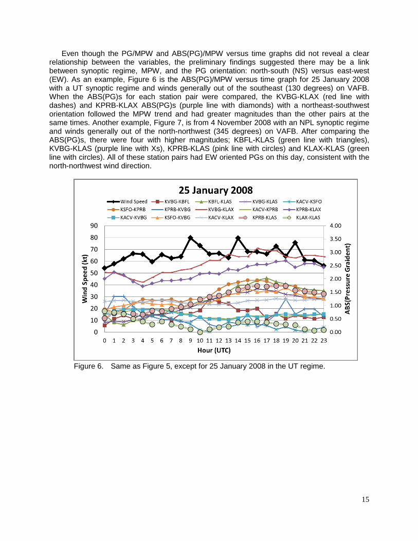
Even though the PG/MPW and ABS(PG)/MPW versus time graphs did not reveal a clear relationship between the variables, the preliminary findings suggested there may be a link between synoptic regime, MPW, and the PG orientation: north-south (NS) versus east-west (EW). As an example, Figure 6 is the ABS(PG)/MPW versus time graph for 25 January 2008 with a UT synoptic regime and winds generally out of the southeast (130 degrees) on VAFB. When the ABS(PG)s for each station pair were compared, the KVBG-KLAX (red line with dashes) and KPRB-KLAX ABS(PG)s (purple line with diamonds) with a northeast-southwest orientation followed the MPW trend and had greater magnitudes than the other pairs at the same times. Another example, Figure 7, is from 4 November 2008 with an NPL synoptic regime and winds generally out of the north-northwest (345 degrees) on VAFB. After comparing the ABS(PG)s, there were four with higher magnitudes; KBFL-KLAS (green line with triangles), KVBG-KLAS (purple line with Xs), KPRB-KLAS (pink line with circles) and KLAX-KLAS (green line with circles). All of these station pairs had EW oriented PGs on this day, consistent with the north-northwest wind direction.

Figure 6. Same as Figure 5, except for 25 January 2008 in the UT regime.

15

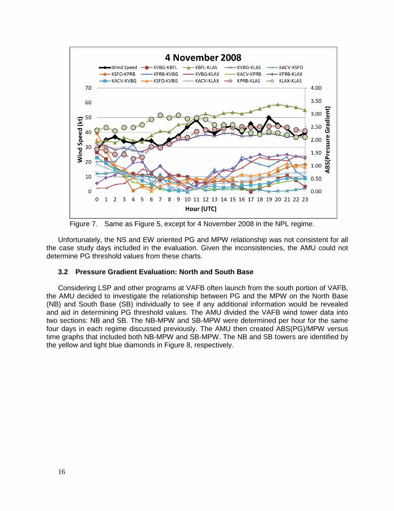
Figure 7. Same as Figure 5, except for 4 November 2008 in the NPL regime.

Unfortunately, the NS and EW oriented PG and MPW relationship was not consistent for all the case study days included in the evaluation. Given the inconsistencies, the AMU could not determine PG threshold values from these charts.

3.2 Pressure Gradient Evaluation: North and South Base

Considering LSP and other programs at VAFB often launch from the south portion of VAFB, the AMU decided to investigate the relationship between PG and the MPW on the North Base (NB) and South Base (SB) individually to see if any additional information would be revealed and aid in determining PG threshold values. The AMU divided the VAFB wind tower data into two sections: NB and SB. The NB-MPW and SB-MPW were determined per hour for the same four days in each regime discussed previously. The AMU then created ABS(PG)/MPW versus time graphs that included both NB-MPW and SB-MPW. The NB and SB towers are identified by the yellow and light blue diamonds in Figure 8, respectively.

16

Figure 8. All VAFB wind towers designated as North Base (yellow) and South Base (light blue).

The AMU compared the NB-MPW and SB-MPW trends to those of the ABS(PG) to see if a stronger qualitative relationship could be found. Figure 9 shows the ABS(PG)/MPW for all towers on VAFB versus time graph for 29 April 2008 with a PH synoptic regime. The MPW is on the left y-axis, the ABS(PG) is on the right y-axis, and time is on the x-axis. Included in the graph are the ABS(PG)s from each of the 14 station pairs used in the task (Table 2). The MPW remains between 40 and 45 kt during the time period until 1000 UTC when it then began a slight upward trend. This same upward trend is not evident in most of the ABS(PG) trends. For instance, the KBFL-KLAS (green line with triangles), KPRB-KLAS (pink line with large outlined circles), KVBG-KLAS (purple line with Xs), and KLAX-KLAS (green line with large outlined circles) ABS(PG)s gradually increased over the entire time period while the KVBG-KBFL ABS(PG) decreased. Figure 10 shows the same ABS(PG) data, but MPW is divided into NB-MPW and SB-MPW. It is clear in this graph that the higher maximum winds on this day were observed on the SB towers. This graph also shows the NB-MPW followed the ABS(PG) trends more closely than the SB-MPW.

17

Figure 9. Example ABS(PG)/MPW versus time graph with PH regime. The MPW is on the left y-axis, the ABS(PG) is on the right y-axis, and time is on the x-axis.

Figure 10. Same as Figure 9 except for NB/SB ABS(PG)/MPW. NB-MPW are the solid black line with diamonds, the SB-MPW are the dashed line with circles.

Unfortunately, these trends were not consistent in other test cases. For example, Figure 11 is a NB/SB ABS(PG)/MPW versus time graph for 22 August 2010 with a PH synoptic regime.

18

Similar to Figure 10, the highest maximum winds were again observed on the SB towers. However, neither the NB-MPW or SB-MPW followed the ABS(PG) trends this day. Another example is shown in Figure 12 from 18 July 2011 with a CL synoptic regime. The SB-MPW gradually increased during the time period while the NB-MPW increased from 0600-1400 UTC and then decreased. The ABS(PG)s from KVBG-KBFL (red line with squares) and KPRB-KVBG (blue line with +s) show the opposite trend where they decreased until 1500 UTC and then experienced a steep increase through the rest of the time period. The remaining ABS(PG)s remained fairly constant or decreased in general. Overall, for the case studies selected, regardless of the time of year or synoptic regime, the NB-MPW and SB-MPW did not follow the same trends as the ABS(PG)s.

Figure 11. Same as Figure 10 except for 22 August 2010.

19

Figure 12. Same as Figure 10 except for 18 July 2011 and for a CL regime.

When creating the NB/SB ABS(PG)/MPW graphs, the AMU noticed most of the maximum winds were observed over the SB portion of VAFB. Of the 28 case study days evaluated, 26 showed SB-MPW values greater than NB-MPW for the majority of the 24-hour time period. The reason is likely due to the elevations of the towers on NB versus SB. At the start of this task the 30 OSSWF provided the AMU detailed information about the VAFB tower network including NB/SB classification, latitude/longitude points and the elevation of each tower. The elevation of each tower is listed in Table 3. The network has 26 towers, 12 on NB and 14 on SB. The elevations of the NB range from 64 to 920 ft while the SB towers range from 27 to 2170 ft. Of the SB towers, five of them have elevations that exceed 1,200 ft. Since wind speeds tend to increase with altitude, the higher altitudes of the SB towers are more likely to observe higher wind speeds. This may impact LSP and other programs that mainly launch from SB on VAFB with vehicles or activities that are sensitive to higher wind speeds. Operations could be delayed or scrubbed if the winds exceed specific constraints.

20

Table 3. List of the 30 OSSWF towers classified by NB/SB and their respective elevations in feet.

North Base South Base

Tower ID Number Elevation Tower ID Number Elevation 0068 459 0070 1446 0069 920 0074 309 0072 125 0077 90 0073 303 0078 450 0075 401 0080 2170 0082 375 0081 296 0083 226 0085 504 0084 120 0086 1200 0089 215 0087 2053 0093 64 0088 27 0096 573 0091 387 0097 330 0092 380

0094 349 0095 1539

3.3 Correlation As previously mentioned, regardless of the time of year or synoptic regime, the analysis

described in section 3.1 did not yield a clear qualitative relationship between PG and MPW for the 28 selected case study days. Given this result, the AMU calculated correlation coefficients between the two variables to quantitatively measure the relationship between them using all days in the 2007-2012 database. The PEARSON function in Microsoft Excel was used to determine the Pearson Correlation Coefficient (PCC). This value is a measure of the linear correlation between two variables ranging from -1 to +1. A result of -1 means there is a perfect negative correlation between the two variables, while a result of +1 means there is a perfect positive correlation. A value of zero indicates there is no relationship between the two datasets.

The AMU calculated this value for each station pair stratified by synoptic regime for the full VAFB, NB and SB towers. Figure 13, Figure 14 and Figure 15 show the ABS(PG) PCC versus synoptic regime for the full base, NB and SB, respectively When comparing the figures, the values in Figure 13 and Figure 15 are nearly identical. This result was expected considering most of the MPWs were observed on the SB towers. When comparing Figure 13 and Figure 14, there are some minor differences among station pairs and corresponding synoptic regimes, but overall the patterns are very similar. These figures show most PCC values range between -0.1 and 0.4 with only a few outliers close to 0.5. Such low values indicate a very weak relationship between ABS(PG) and MPW at VAFB and should not be the lone data source when forecasting MPW.

21

Figure 13. ABS(PG) PCC versus synoptic regime for the full base from 2007-2012. The solid black line highlights where PCC equals zero. The PCC is on the y-axis and the synoptic regime on the x-axis. The “ALL” category on the x-axis includes all of the days in the 2007-2012 database regardless of synoptic regime and the solid black horizontal line highlights where PCC equals zero.

Figure 14. Same as Figure 13 except for NB towers.

22

Figure 15. Same as Figure 13 except for SB towers.

The tool currently used by the 30 OSSWF to predict MPW examines dP between the station pairs instead of PG. As a comparison, the AMU created a graph displaying the dP PCC versus synoptic regime for the full base (Figure 16). Compared to the ABS(PG) PCC results, dP PCC has a smaller range per synoptic regime and values closer to zero. The North Pacific High (NPH) and PH regimes show the highest PCC values however, they are mainly between zero and 0.5 with the exception of KVBG-KBFL in PH where PCC is -0.14. This graph confirms dP also performs poorly as a predictor for MPW at VAFB.

Given these PCC values and those of the PG evaluations described in sections 3.1 and 3.2, the AMU was unable to determine PG thresholds or trends that could be used to forecast warning-level winds in the VAFB wind tower network.

23

Figure 16. Same as Figure 13 except for dP.

4 Summary Warning category winds can adversely impact day-to-day space lift operations at VAFB in

California. NASA’s LSP and other programs at VAFB use wind forecasts issued by the 30 OSSWF to determine if they need to limit activities or protect property such as a launch vehicle. The 30 OSSWF tasked the AMU to develop an automated Excel GUI that includes PG thresholds between specific observing stations under different synoptic regimes to aid forecasters when issuing wind warnings. This required an analysis to determine if relationships between the MPW and PG trends and threshold values existed. To conduct the analysis, the AMU obtained historical VAFB wind tower and regional MSLP observations. The 30 OSSWF delivered all available data from their 26 VAFB wind tower network in the period October 2007–November 2012. The AMU processed the observations and then developed a database containing MPWs for each tower and day in the dataset. The AMU identified all days where peak winds ≥ 40 kt were observed and provided a list of these dates to the 30 OSSWF for them to stratify by synoptic regime. The 45 WS obtained MSLP observations from the seven regional weather stations identified by the 30 OSSWF from the 14 WS to calculate the PGs. Once received, the AMU developed an MSLP database containing hourly observations from each station on the days when peak winds ≥ 40 kt were observed. These observations were also stratified by synoptic regime and the hourly PGs for each station pair were calculated.

In order determine if relationships exist between MPW at VAFB and PG trends and/or values, the AMU created a series of graphs plotting ABS(PG) and MPW versus time for four days in each of the seven synoptic regimes, each day representing a different time of the year in order to have a diverse collection of case studies. The initial review of the ABS(PG)s and MPW did not yield a clear relationship between the two variables. For the days selected, most ABS(PG) trends did not follow the MPW trends. The AMU investigated the potential relationship between PG orientation and MPW but found it was inconsistent. Considering these results, and that LSP mainly launches out of the SB portion of VAFB, the AMU further investigated the PG and MPW relationship by dividing VAFB into two sections: NB and SB. The NB-MPW and SB-MPW were determined per hour for the same four days in each regime discussed previously and ABS(PG)/MPW versus time graphs were created, including graphs for NB-MPW and SB-

24

MPW. Unfortunately, for the 28 selected case study days, stratifying VAFB this way did not reveal a stronger qualitative relationship between PG and MPW regardless of the time of year or synoptic regime, therefore PG threshold values could not be determined.

The AMU then calculated correlation coefficients between PG and MPW to quantitatively measure the relationship between them using all days in the 2007-2012 database. These values were calculated for each station pair stratified by synoptic regime for the full VAFB, NB and SB. Most PCCs ranged between -0.1 and 0.4 with very few outliers near 0.5. Such low PCC values show a very weak relationship between PG and MPW at VAFB. Therefore, PG should not be the lone data source when forecasting MPW. Based on the subjective PG review of trends and values and the objective PCC values, the AMU determined there was no relationship between PG and MPW and therefore did not develop an automated GUI for the 30 OSSWF.

25

List of Acronyms 14 WS 14th Weather Squadron

30 OSSWF 30th Operational Support Squadron Weather Flight

45 WS 45th Weather Squadron

ABS Absolute Value

AMU Applied Meteorology Unit

CH California High

CL California Low

dP Pressure Difference

EW East-West

GBH Great Basin High

GUI Graphical User Interface

MPW Maximum Peak Wind

MSLP Mean Sea Level Pressure

NB North Base

NPH North Pacific High

NPL North Pacific Low

NS North-South

PCC Pearson Correlation Coefficient

PG Pressure Gradient

PH Pacific High

SB South Base

UT Upper Trough

VAFB Vandenberg Air Force Base

26

NOTICE Mention of a copyrighted, trademarked or proprietary product, service, or document does not constitute endorsement thereof by the author, ENSCO Inc., the AMU, the National Aeronautics and Space Administration, or the United States Government. Any such mention is solely for the purpose of fully informing the reader of the resources used to conduct the work reported herein.

27