3. Micro-statics, Micro comparative statics and Micro Dynamics

On the basis of time, the equilibrium between two variables in microeconomics is divided into three parts as micro statics, comparative and dynamic which are also called types of microeconomics. The types of Microeconomics is explained separately as stated below;

4. Micro staticsMicro statics refers to the stationary

situation of the equilibrium between different variables at certain point of time. In other words, when the value of economic variables are related to the same point of time, the functional relationship between variables is said to be statics.

It is expressed as The equilibrium condition of a particular point in

time is

Where,

The concept of micro statics has been illustrated in the following figure as;

The figure shows the equilibrium of the market in a certain point of time. Both the demand curve DD and supply curve SS have intersected each other at point E in a particular point in time. So E is the point of equilibrium which relates two of the variables price (OP) and quantity (OQ) at a particular point in time. This is a static analysis

Y

X

S

S

D

D0 Q

P

Price

Quantity

E

2- Comparative Micro statics

As time passes, there is change in the condition of demand and supply. This change in demand and supply brings a change even in the equilibrium condition. This type of change in equilibrium at different points of time is the study of comparative micro statics. Therefore comparative micro statics is the study of different equilibriums at different points of time.

Comparative micro statics compares one equilibrium with other equilibrium but it does not study about the process how one equilibrium breaks and another equilibrium establishes. The comparative micro static can also be shown in the figure below as,

In the figure E is the initial equilibrium, where equilibrium price is OP and equilibrium quantity is OQ. When the demand rises from DD toD1D1, the new equilibrium shifted from E to E1 where the equilibrium price is OP1 and equilibrium quantity is OQ1. The comparative study of the two equilibrium points E, E1 is the comparative micro statics but this study does not explain about the process how a new equilibrium attains.

Y

X

S

S

D

D

0 Q

PPrice

Quantity

E

E1P1

D1

D1

Q1

3-Micro dynamicsThere is always change in time. This change brings

change in price and the demand & supply of quantity of commodities. Consequently there is a change in equilibrium. Therefore micro dynamics refers to that situation of equilibrium in which an equilibrium of different variables goes through disequilibrium and new equilibrium establishes. Hence micro dynamics is the study of the process which shows how the initial equilibrium breaks and new equilibrium attains. Micro dynamics can also be explain by the following figure.

In the figure, E is the initial point of equilibrium at which 0P1 piece & 0Q1 quantity are the equilibrium price & equilibrium quantity. Now let us suppose that there is an increase in income at given price 0P1. The increase in income causes a shift in demand curve from DD to D1D1. This brings about a disequilibrium in the market and the series of disequilibrium persists until the new equilibrium

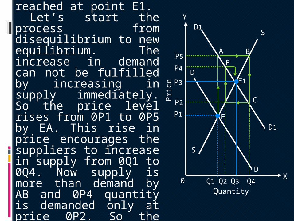
reached at point E1. Let’s start the process

from disequilibrium to new equilibrium. The increase in demand can not be fulfilled by increasing in supply immediately. So the price level rises from 0P1 to 0P5 by EA. This rise in price encourages the suppliers to increase in supply from 0Q1 to 0Q4. Now supply is more than demand by AB and 0P4 quantity is demanded only at price 0P2. So the price falls from 0P5 to 0P2. This fall in price causes a fall in supply from 0Q4 to 0Q2 or the supply is equal to 0Q2.

FD

S

S

X

Y

E1

E

BA

D1

D1

D

C

0 Q1 Q2 Q3 Q4

Quantity

Pric

e

P5

P4

P3

P2

P1

But demand is still higher than supply which pushes the price up from 0P2 to 0P4. Again the supplier are encouraged to increase in supply. This process continues again & again until the final point of equilibrium is reached at price 0P3 & quantity at 0Q3.

This is how micro dynamics explain about the process how an equilibrium breaks and another new point of equilibrium establishes.

In the figure E is the initial point of equilibrium.

0P1 is the determined price.

0Q1 is the determined quantity

P

S

S

Q0

EP1

Q1

D

D

Let us suppose that there is a change in some independent variable. Say, income increases. As a result demand for the commodity extended. This causes a shift in demand curve upwards from DD to D1D1. Consequently, new point of equilibrium stablishes at point E1.

P

S

S

Q0

EP1

Q1

D

D

D1

D1

E1

But supply can not be increase immediately to fulfill increased demand for the commodity. As a result price goes up from 0P1 to 0P5 but quantity supplied remains equal to 0Q1 in the first round of supply.

P

S

S

Q0

EP1

Q1

D

D

AD1

D1

E1

P5

Due to rise in the price, the producer, encourages to produce more and supply more than before in the second round of supply. They supply the commodity equal to 0Q4 at 0P5 price.

But what about the consumer? Are the ready to pay 0P5 to absorb whole supply?

P

S

S

Q0

EP1

Q1

D

D

AD1

D1

E1

P5B

Q4

P

S

S

Q0

EP1

Q1

D

D

AD1

D1

E1

P2

B

Q4Q2

P5

GC

No, the consumers are ready pay the price only 0P2 for 0Q4 quantity because of over supply. So the price goes down to 0P2.

The fall in price is responded by the producers with a cut in supply or they want to supply only 0Q2 quantity at 0P2 price.

This amount of supply is still less than the equilibrating quantity of demand. So the price again goes up at quantity supplied equal to 0Q2.

P

S

S

Q0

EP1

Q1

D

D

AD1

D1

E1

P2

B

Q4Q2

P5

P4F

CG

The price rises up to 0P4 at 0Q2 quantity supplied. This rise in price again encourages the producer to increase in supply. As a result the supply goes up in the next round.

The supply is again excess than the equilibrating amount of demand. So the price goes down again but not so much as it was before.

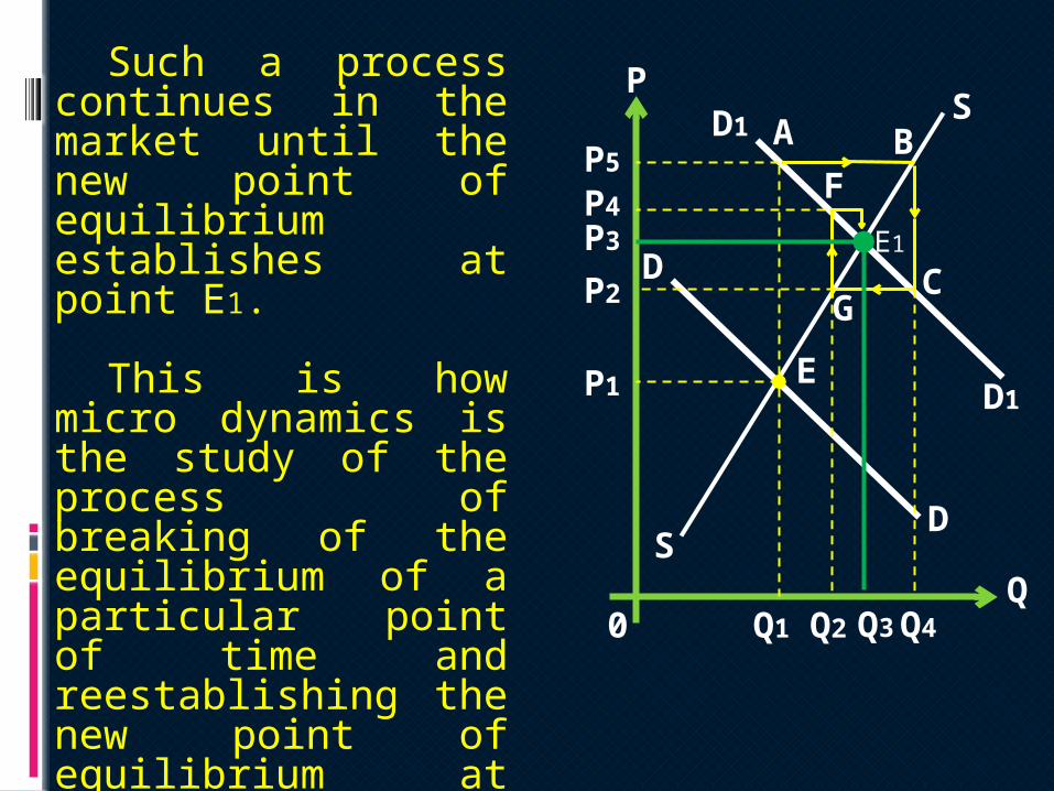
Such a process continues in the market until the new point of equilibrium establishes at point E1.

This is how micro dynamics is the study of the process of breaking of the equilibrium of a particular point of time and reestablishing the new point of equilibrium at other particular point of time.

Thank You !

P

S

S

Q0

EP1

Q1

D

D

AD1

D1

E1

P2

B

Q4Q2

P5

P4

Q3

F

CG

P3